


ABSTRACT
In this study, the photospheric vector magnetograms, obtained with the Spectro-Polarimeter of the Solar Optical Telescope on board Hinode, are used as the boundary conditions to extrapolate the three-dimensional nonlinear force-free (NLFF) coronal magnetic fields. The observed non-force-free photospheric magnetic fields are preprocessed toward the nearly force-free chromospheric magnetic fields. The performance of the preprocessing procedure is evaluated by comparing with chromospheric magnetic fields obtained by the Vector SpectroMagnetograph instrument located on the Synoptic Optical Long-term Investigations of the Sun Tower. Then, the weighted optimization method is applied to the preprocessed boundary data to extrapolate the NLFF fields with which we are able to estimate the free magnetic energy stored in the active regions. The magnitude scaling correlation between the free magnetic energy and the soft X-ray flare index (FI) of active regions is then studied. The latter quantifies the impending flare production of active regions over the subsequent 1, 2, and 3 day time windows. Based on 75 samples, we find a positive correlation between the free energy and the FI. We also study the temporal variation of free magnetic energy for three active regions, of which two are flare-active and one is flare-quiet during the observation over a period of several days. While the magnitude of free magnetic energy unambiguously differentiates between the flare-active and the flare-quiet regions, the temporal variation of free magnetic energy does not exhibit a clear and consistent pre-flare pattern. This may indicate that the trigger mechanism of flares is as important as the energy storage in active regions.
Export citation and abstract BibTeX RIS
1. INTRODUCTION
The solar magnetic field is the source of most (if not all) solar energetic events such as flares and coronal mass ejections (CMEs). Since the coronal magnetic fields cannot be precisely measured at present except in a few special cases (e.g., Gary & Hurford 1994; Lin et al. 2004), the efforts to identify the magnetic properties important for flare/CME production have been made almost exclusively with parameters derived from the photospheric magnetic fields. Generally speaking, these magnetic parameters quantify the size and/or the topological complexity of an active region. Several recently identified properties are: the total unsigned magnetic flux Φ = ∫|Brad|dA, where Brad is the radial component of the magnetic field and the integral is performed over the field of view (FOV) A (Barnes & Leka 2008; Song et al. 2009); the amount of magnetic flux close to the strong-gradient magnetic polarity inversion line (PIL; Schrijver 2007); the length of the high-gradient and high-sheared PIL (Falconer et al. 2003); the total magnetic dissipation (Jing et al. 2006; Song et al. 2009); the effective connected magnetic field (Georgoulis & Rust 2007); and the photospheric excess energy (Leka & Barnes 2003; Barnes & Leka 2008). In particular, the photospheric excess energy Epe measures the difference between the observed and the potential fields (i.e., the current-free fields, computed from the vertical component of magnetic fields) at the photospheric surface, i.e.,  , where the superscripts o and p represent the observed field and the potential field, respectively. Note that Epe is not truly magnetic energy stored in an active region, since the integral is computed only at the photospheric surface and not throughout the coronal volume. Although all these photospheric magnetic parameters have been reported to bear a certain relation to flare occurrence, the limitations of using the state of photospheric magnetic fields to distinguish between flare-active and flare-quiet regions and to forecast flare occurrences have been addressed (Leka & Barnes 2007).
Compared with those photospheric magnetic parameters, free magnetic energy Efree derived from three-dimensional coronal magnetic configuration over an active region seems to be a more intrinsic physical parameter related to the flare/CME productivity of an active region. Efree quantifies the energy deviation of the coronal magnetic field from its potential state. Since the coronal magnetic field is commonly referred to as nonlinear force-free (NLFF) field, Efree can be estimated by
where V is the volume of the computational domain from photosphere to corona, and the superscripts N and p represent the NLFF field and the potential field, respectively. Efree calculated in this way is regarded as the upper limit of the energy that is available to power the flares/CMEs. Knowledge of the amount of Efree and its temporal variation associated with flares/CMEs is important to our understanding of energy storage and release processes in active regions. Progress in this research area has been made recently by, e.g., Bleybel et al. (2002), Régnier et al. (2002), Régnier & Canfield (2006), Guo et al. (2008), Thalmann & Wiegelmann (2008), Thalmann et al. (2008), and Jing et al. (2009).
On the other hand, solar flares are classified as X, M, C, or B according to their peak soft X-ray (SXR) flux, as measured by the Geostationary Operational Environmental Satellite (GOES) and recorded in the NOAA Space Environment Center's solar event reports. The peak SXR flux of X-, M-, C-, and B-class flares is of 10−4, 10−5, 10−6, and 10−7 W m−2 magnitude order, respectively. As proposed by Abramenko (2005), the flare productivity of an active region can be measured by the SXR flare index (FI, hereafter) which counts the X-, M-, C-, and B-class flares by different weights. The weight of each class is 10 times stronger than the succeeding one, with X-class flares having a weight of 100 in units of  , i.e.,
where τ is the length of the time window, usually measured in days, and IX, IM, IC, and IB are GOES peak SXR flux of X-, M-, C-, and B-class flares produced by the given active region within the time window τ. In other words, the FI measures an active region's daily average flare production within the time window. In this study, we use three different time windows ranging from the time of the analyzed magnetogram to 1, 2, and 3 subsequent days after that time, i.e., FIn−day, where n = 1, 2, 3.
The goal of this paper is twofold. First, we examine the statistical correlation between free magnetic energy Efree derived from three-dimensional NLFF fields and FI measured within the 1, 2, and 3 time windows FIn−day. To our knowledge, this correlation has not been explored before. Second, we study the temporal variation of Efree for both flare-active and flare-quiet regions. With the advances in the high-resolution vector-magnetographic capabilities of the Hinode spacecraft (Kosugi et al. 2007) and the computational capabilities of NLFF field extrapolation, we are presently in a good position to explore these issues. We anticipate that this study will help us disclose the energy storage and release mechanism of flares, and perhaps even provide a tool to forecast flares.
2. DATA PROCESSING AND NLFF FIELD EXTRAPOLATION
This study requires extrapolating the three-dimensional NLFF coronal fields from the photospheric boundary. The photospheric vector magnetograms, obtained by the Spectro-Polarimeter (SP) of the Solar Optical Telescope (SOT; Tsuneta et al. 2008) on board Hinode, are used as the boundary conditions. The SOT-SP obtains Stokes profiles of two magnetically sensitive Fe lines at 630.15 and 630.25 nm with a sampling of 21.6 mÅ. The polarization spectra are inverted to the photospheric vector magnetograms using an Unno–Rachkovsky inversion based on the assumption of the Milne–Eddington atmosphere (e.g., Lites & Skumanich 1990; Klimchuk et al. 1992). We use this data set solely, because it has the best polarization accuracy and seeing free condition to provide needed consistency in this statistical study.
The 180° azimuthal ambiguity in the transverse magnetograms is resolved using the "minimum energy" method that is the top-performing automated method among state-of-art algorithms in this area (Metcalf et al. 2006). This method uses the simulated annealing algorithm to minimize a function  , where the former is the vertical electric current density and the latter is the field divergence (Metcalf 1994). The projection effects are removed by transforming the observed vector magnetograms to heliographic coordinates, i.e., the heliographic-Cartesian x-, y-, and z-components.
The NLFF field extrapolation endeavors have been plagued by the problem that the photospheric magnetic field, which has a plasma-β of the unity order, does not satisfy the force-free condition (Gary 2001). To find suitable boundary conditions for the NLFF field modeling, we have to preprocess the measured photospheric magnetograms by using a preprocessing scheme developed by Wiegelmann et al. (2006). This preprocessing scheme removes forces and torques from the boundary and approximates the photospheric magnetic field to the low plasma-β force-free chromosphere. In an effort to test the performance of the preprocessing procedure, we compare the unpreprocessed and preprocessed SOT-SP photospheric line of sight (LOS) magnetogram Bz of AR NOAA 10930 with the co-aligned LOS chromospheric magnetogram when the active region is close to the disk center. The chromospheric magnetogram was obtained by the Vector SpectroMagnetograph (VSM) instrument located on the Synoptic Optical Long-term Investigations of the Sun (SOLIS; Keller & NSO Staff 1998). SOLIS/VSM produces spectroheligram of He i line at 1083.0 nm, photospheric LOS and vector magnetograms of Fe line at 630.2 nm, and chromospheric LOS magnetograms of Ca ii line at 854.2 nm line. The latter are used here for comparison. The comparison is made on a pixel-by-pixel basis and the scatter plots are shown in Figure 1. As seen from this figure, the linear correlation coefficient (CC) increases from 0.78 to 0.93 in the unpreprocessed to preprocessed case, indicating that the preprocessed field is closer to the chromospheric field, and hence closer to the force-free condition. Additionally, as confirmed by some model tests (Metcalf et al. 2008; Wiegelmann et al. 2008), the ability of the NLFF field extrapolation algorithms to reconstruct the coronal field morphology is substantially improved by using the preprocessed photospheric boundary.
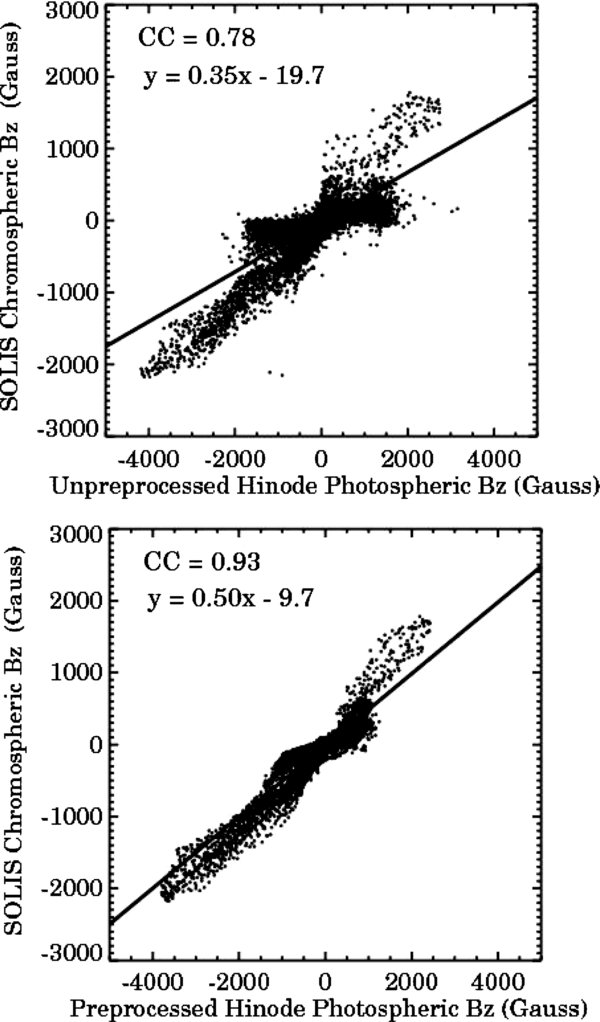
Figure 1. Top: SOLIS chromospheric LOS magnetic field Bz vs. unpreprocessed Hinode/SP photospheric Bz; bottom: SOLIS chromospheric Bz vs. preprocessed Hinode/SP photospheric Bz. The SOLIS chromospheric magnetogram was taken on 2006 December 11 at 18:15 UT in AR 10930, and the Hinode/SP photospheric magnetogram was taken at 17:00 UT on the same day and in the same active region. The solid line in each panel is the least-square best fit to the data points in a form of y = ax + b, where a and b are constants. The linear CCs between the quantities are shown in each panel.
Download figure:
Standard image High-resolution imageFinally, the NLFF field and the potential field were extrapolated from the disambiguated and preprocessed magnetograms using the weighted optimization method (Wiegelmann 2004) and Green's function method (Aly 1989), respectively. The weighted optimization method is an implementation of the original work of Wheatland et al. (2000). It involves minimizing a joint measure (L) for the normalized Lorentz force and the divergence of the field throughout the computational domain V:
where  , ωf and ωd are weighting functions for the force and divergence terms, respectively. Both ωf and ωd are position dependent. They are chosen to be 1.0 in the center of the computational domain and drop to 0 monotonically in a buffer boundary region that consists of 16 grid points toward the side and top boundaries. More detailed descriptions of the method were given by Wiegelmann (2004) and Schrijver et al. (2006). Subsequently, we derived free magnetic energy Efree using the integration Equation (1) over the three-dimensional volume.
3. DESCRIPTION OF ACTIVE REGIONS
Hinode was launched in 2006 September and the SOT-SP on board Hinode captured its first light on 2006 October. A total of 97 active regions were identified by NOAA from 2006 October 1 to 2008 December 31, i.e., NOAA 10913-11009. Of these active regions, during their lifetime, a considerable part (73 of 93) did not produce any flare activity above B-class (referred to as "flare-quiet"), 21 produced moderate flares (C-class), and three produced major flares (X- and/or M-class).
To check the statistical correlation between Efree and FIn−day, it is important that the sample is comprised major flaring, moderate flaring, and flare-quiet regions. Therefore, we give priority to NOAA 10930 and 10960, as they are two of the very few active regions which produced major flares. Moreover, NOAA 10930 and 10960 are well covered by the SOT-SP observation over a period of several days. The data taken at both flare-active and flare-quiet phases not only expand the sample size but also diversify the values of FIn−day. Additionally, another 11 active regions are included in the sample to supplement the low end of FIn−day. The data selection is mainly based on the availability of the SOT-SP data. A final tally of 75 vector magnetograms from 13 active regions are analyzed in this paper. All the vector magnetograms analyzed in this study are within ±45° in longitude and ±30° in latitude. The distribution of FI3−day shows that 33 of 75 (44%) cases lie between 0 and 1 (i.e., flare quiet during the subsequent 3 day time window), 27 of 75 (36%) cases lie between 1 and 10 (equivalent to a daily average of a C-class flare during the subsequent 3 day time window), and the rest 15 (20%) cases are larger than 10 (equivalent to a daily average of a M/X-class flare during the subsequent 3 day time window). Table 1 lists the information on the 13 active regions.
Table 1. Information of Active Regions
| Index | NOAA | Number Of | Maximum Flare Magnitude | Dimensions of V a | FIoverallb |
|---|---|---|---|---|---|
| Frames | During Lifetime | (Mm3) | (10−6 W m−2) | ||
| 1 | 10930 | 25 | X3.4 | 210 × 115 × 87 | 112.7 |
| 2 | 10960 | 15 | M1.0 | 210 × 115 × 87 | 18.1 |
| 3 | 10921 | 1 | C3.7 | 104 × 104 × 87 | 0.4 |
| 4 | 10923 | 1 | C3.3 | 73 × 87 × 87 | 1.1 |
| 5 | 10933 | 1 | C1.7 | 136 × 115 × 87 | 0.6 |
| 6 | 10938 | 1 | C4.2 | 136 × 115 × 87 | 0.9 |
| 7 | 10940 | 1 | C3.4 | 115 × 115 × 87 | 1.0 |
| 8 | 10953 | 1 | C8.5 | 104 × 104 × 87 | 1.1 |
| 9 | 10956 | 1 | C2.9 | 112 × 112 × 87 | 0.7 |
| 10 | 10963 | 25 | C8.2 | 210 × 112 × 87 | 3.2 |
| 11 | 10978 | 1 | C4.5 | 108 × 108 × 87 | 1.6 |
| 12 | 10961 | 1 | None | 115 × 115 × 87 | 0.0 |
| 13 | 11005 | 1 | None | 108 × 108 × 87 | 0.0 |
Notes. aV: the volume of computational domain, see Equation (1). bFIoverall is calculated with Equation (2), the time window τ is the lifetime of the active regions.
Download table as: ASCIITypeset image
As shown in the fifth column of the Table 1, the heights of the computational domain are chosen to be 87 Mm above the photosphere for all the cases, but the FOVs on the lower boundary vary from case to case according with the SOT-SP scan area. Since Efree is a volume-integrated parameter, the difference in the lower boundary FOVs may introduce an uncertainty in the statistical correlation and must be treated with caution.
Figure 2 presents an example in which we test how Efree of an active region changes with the varying FOV and height of the computational domain V. The top panel in Figure 2 shows a LOS magnetogram of the active region NOAA 10930. The colored boxes mark the nine different FOVs, ranging from 22 × 9 Mm2 to 210 × 115 Mm2. The smallest box only covers a small area around the flaring PIL, while the largest box covers not only the sunspots that comprise the major portion of this active region but also the weaker plage regions surrounding the sunspots. The bottom left panel shows the NLFF field energy EN, the potential field energy Ep, and the free magnetic energy Efree as a function of the nine selected FOVs, given a fixed height (87 Mm) of the computational domain V. As shown in Equation (1), Efree is defined as the excess EN from Ep. Each data point with a certain color corresponds respectively to the FOV box with the same color. We see that Efree first increases rapidly with an expanding FOV, then reaches its maximum when the major portion of this region is covered by the FOV, then changes little despite the continued growth of FOV. The bottom right panel shows EN, Ep, and Efree as a function of height of the upper boundary of V, given a fixed FOV (210 × 115 Mm2) of the lower boundary. Evidently, Efree displays an impulsive increase from the lower boundary to a certain height (∼25 Mm in this case), then stays almost constant beyond this height. We run the Efree–FOV and Efree–height tests on other active regions and get similar results. It suggests that the difference in FOVs of our samples is not likely to significantly affect the statistical correlations that will be shown in Section 4, as long as the sampled active regions are well covered by the magnetograms. It also suggests that the magnetic fields approach potential beyond a certain height which is of a few tens of Mm magnitude order, consistent with our previous results (Jing et al. 2008). A height of 87 Mm of V adopted in this study seems to be enough to constrain the nonpotential magnetic fields.

Figure 2. Top: snapshot of LOS magnetograms of NOAA 10930. The whole FOV is 210 Mm × 115 Mm. The colored boxes mark the nine different FOVs. Bottom left: NLFF field energy EN, potential field energy Ep, and free magnetic energy Efree as a function of the nine selected FOVs, given a fixed height of the upper boundary (87 Mm). The data dot with a certain color corresponds respectively to the FOV box with the same color. Bottom right: EN, Ep, and Efree as a function of height of the upper boundary, given a fixed FOV of 210 Mm × 115 Mm.
Download figure:
Standard image High-resolution imageTo study the temporal variation of Efree, we select three active regions, NOAA 10930, 10960, and 10963. As mentioned, the former two exhibited one major flare and several moderate flares during the SOT-SP observations over a period of days. The latter produced a few moderate flares at some point in its lifetime, but did not flare during the observation period. For each region, a sequence of the vector magnetograms at a general cadence of a few hours is used as the boundary conditions to extrapolate the three-dimensional NLFF field. These magnetograms are de-projected, co-aligned, and rescaled so that they have the same target location, the same FOV, and the same dimensions. In Figure 3, the snapshots of the vector magnetogram of the three regions and the corresponding NLFF fields are shown in the left and right columns, respectively.

Figure 3. Left panels: snapshots of the Hinode/SP vector magnetograms. From top to bottom, they are NOAA 10930 taken on 2006 December 11 at 11:10 UT, NOAA 10960 taken on 2007 June 6 at 12:30 UT, and NOAA 10963 taken on 2007 July 13 at 19:07 UT. The background images are the LOS magnetograms. Green arrows indicate the transverse fields. The FOVs of three magnetograms are 210 Mm × 115 Mm, 210 Mm × 115 Mm, and 210 Mm × 112 Mm, respectively. Right panels: extrapolated NLFF fields of NOAA 10930, 10960, and 10963. The boundary images are the vector magnetograms shown in the left panels.
Download figure:
Standard image High-resolution image4. RESULTS
In Figure 4, the left-to-right top panels show the scatter plots of FI3−day versus Efree, FI2−day versus Efree, and FI1−day versus Efree, respectively. The solid line superposed in each plot indicates the least-square best fit to the data points. The cross CCs between the quantities are also given in the panels. Note that FIn−day is plotted in a logarithmic scale. The FIn−day with 0 value is set to 0.01 to avoid arithmetic error and is shown as gray points. These gray points are excluded from the fitting and CC calculation. While the points are widely scattered, the result still reveals a positive correlation between the quantities (0.55 < CCs < 0.76), suggesting that major flares generally come from active regions with high-energy content.
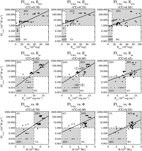
Figure 4. Top panels: scatter plots of FIn−day vs. Efree; middle panels: scatter plots of FIn−day vs. Epe; bottom panels: scatter plots of FIn−day vs. Φ, where n = 3, 2, 1 from left to right. The FIn−days with 0 value are set to 0.01 to avoid arithmetic error and shown as gray points. The solid lines indicate the least-square best fits to the data points, and CCs are CCs, with gray points excluded. In each panel, the data points are divided into four groups, denoted by (1)–(4) in the middle panel, with the horizontal and vertical dashed lines. The horizontal dashed line shows FIn−day = 1, while the vertical dashed line is drawn according with the maximum Efree of the flare-quiet regions. The percentages refer to the frequencies of each group.
Download figure:
Standard image High-resolution imageFurthermore, to test the ability of Efree to distinguish between flare-quiet and flare-active populations, we divide the data points into four groups (denoted by 1–4, seen in the middle panel of Figure 4) with the horizontal and vertical dashed lines in each panel. The horizontal dashed line shows the observed FIn−day = 1, which is equivalent to a daily average of a C1.0 flare within the time window and is taken as a threshold for flare-active regions. The vertical dashed line is drawn according with the derived maximum Efree of the flare-quiet regions. We wish to test the hypothesis that the population on the right side of the vertical line are flare active. In this sense, group 1 refers to incorrectly rejected flare-active cases (Type I error) and group 2 refers to failing to reject the flare-quiet cases (Type II error). Groups 3 and 4 (the shaded areas) mean that flare-quiet and flare-active populations are well separated by the vertical line. The frequencies of the groups 1–4 are also given in Figure 4. Inspection of Figure 4 immediately reveals that most of data points fall into groups 3 and 4. The Type I and Type II error rates are ∼8%–12% in total. This means that, based on the sample presented here, flare-quiet and flare-active populations can be separated by Efree with a ∼88%–92% success rate.
For comparison, the middle and bottom panels of Figure 4 show similar diagrams in which the photospheric excess energy Epe and the total unsigned photospheric magnetic flux Φ are plotted against the FIn−day. The definitions of Epe and Φ are given in Section 1. The former is regarded as a proxy for Efree, while the latter is a simple measure of an active region's size (Barnes & Leka 2008). The positive correlations are still evident in each panel. We also note the following properties.
First, when two populations (flare quiet and flare active) are concerned, Φ and Efree perform better than Epe in separating two populations. Taking the 3 day time window, for example, the success rates of Φ, Efree, and Epe are 95%, 90%, and 77%, respectively.
Second, when only considering the flare-active population, all three parameters are moderately to strongly correlated with FIn−day. In addition, despite the fact that Efree is one of the most direct measures for the available energy in a three-dimensional magnetic field, its correlations with FIn−day are found to be quite similar to the correlations of the photospheric magnetic parameters, Epe, and Φ. In particular, Epe performs best in relating to FI3−day with a CC as high as 0.82 and performs worst in relating to FI1−day with a CC of 0.45. Basically, the difference among these three parameters is not significant. The similar magnitudes of the CCs imply that Efree, Epe, and Φ have approximately equal predictability for flares.
Finally, as a general trend, the magnitude of the CCs decreases as the time window of FI becomes narrower from 3 days to 1 day. It reveals that the magnetic parameters have relatively less predictability for flares within a 1 day time window than a 3 day time window. It is understandable, because flares as a result of electromagnetic instabilities may occur only under certain circumstances and after a substantial waiting time (Schrijver et al. 2005). Forecasting imminent flares certainly faces more uncertainties than forecasting long-term flares.
Figure 5 illustrates how three magnetic parameters, Efree, Epe, and Φ, correlate with each other. The colored data points from dark to light refer to increasing levels of FI3−day from flare quiet to major flaring. Apparently, the major flaring samples generally exhibit higher values of Efree, Epe, and Φ than the flare-quiet ones. It is interesting to note that, the data points of Efree–Φ in the top panel can be fitted by two lines with different slopes. The lower line mainly contains the data from flare-quiet samples, while the higher line is comprised data from two major flaring active regions (NOAA 10930 and 10960) that were observed on a timescale of several days. Epe does not exhibit such a pattern with Φ. The result suggests that Φ is fairly constant for major flaring regions, but Efree may change significantly over days. It is not very surprising, because Efree, as a difference between the NLFF field and the potential field, should be expected to be intrinsically more variable than Φ. In addition, the correlation between Efree and Φ is weak (CC=0.3) for flare-quiet samples, but very strong (CC=0.86) for flare-active ones.
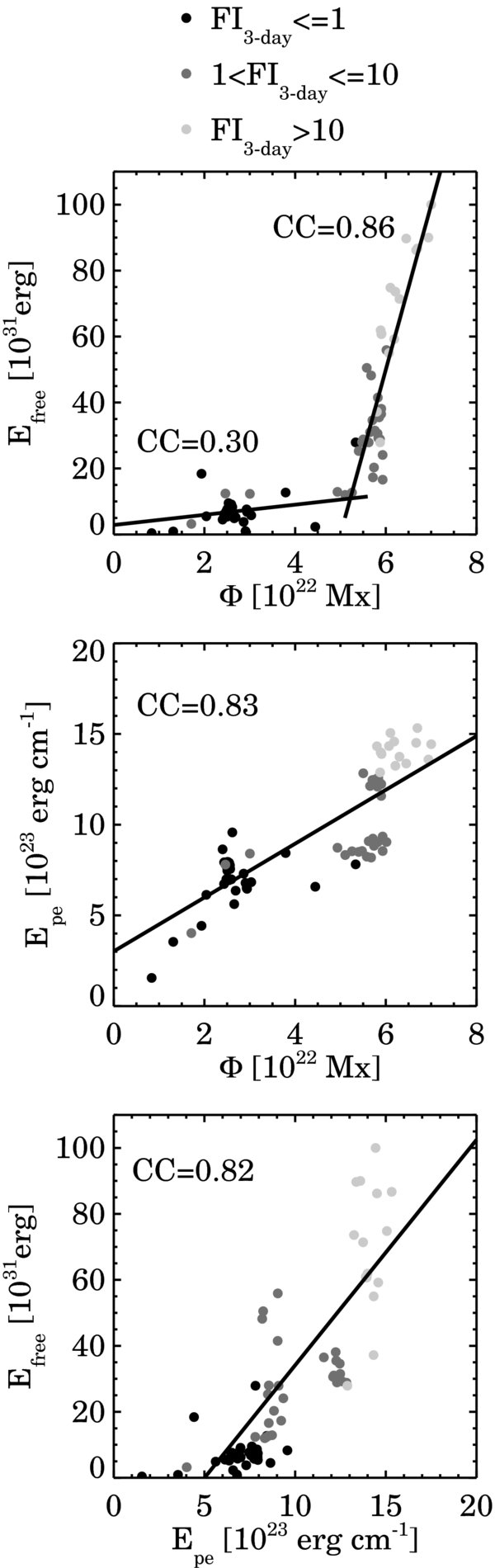
Figure 5. Top panels: Scatter plots of Efree vs. Φ; Middle panels: Scatter plots of Epe vs. Φ; Bottom panels: Scatter plots of Efree vs. Epe. The solid lines are the least-square best fits to the data points, and CCs are CCs. The different colors of the data points refer to the different levels of the flare activity within the subsequent 3 days.
Download figure:
Standard image High-resolution imageTheoretically speaking, the statistical relation between Efree and FIn−day and the temporal variation of Efree derived from individual active regions can provide clues to distinguish between flare-active and flare-quiet regions. We compare the long-term variation of Efree for three active regions, NOAA 10930, 10960, and 10963. Figure 6 shows the time profiles of Efree (gray histogram), Epe (green diamonds), Φ (blue pluses), and the GOES SXR 1–8 Å light curves (red curves). The flares that originated from the active regions are indicated by the black arrows. As shown in Figure 6, NOAA 10930 dominated the solar activity during the observation from 2006 December 9–14 and produced a X3.4 flare on 2006 December 13. Efree in NOAA 10930 is remarkably built up during the 2 day prior to the X3.4 flare and even continues to increase after the flare. NOAA 10960 is also flare active. It produced a M1.0 flare on 2007 June 9, at the very end of our observation and four C-class flares during the observation. Efree in NOAA 10960 fluctuates and does not have any obvious association with the flare occurrence. NOAA 10963 did not flare during the observation from 2007 July 12 to 16 and contains a clearly lower amount of Efree in comparison with the other two regions. Since the long-term trend of Efree varies from case to case, we find no particular pre-flare signatures useful in predicting flares.
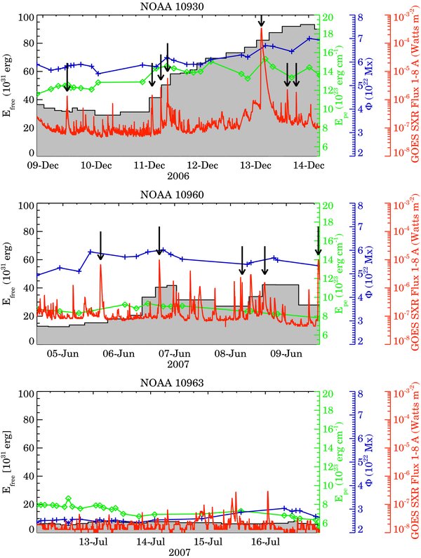
Figure 6. Temporal variation of free magnetic energy Efree (gray histograms), photospheric excess energy Epe (green diamonds), the photospheric unsigned magnetic flux Φ (blue pluses), and the GOES SXR 1–8 Å light curves (red curves) of NOAA 10930, 10960, and 10963. The flares that originated from the active regions are indicated by the black arrows.
Download figure:
Standard image High-resolution image5. QUALITY CONTROL AND UNCERTAINTY ANALYSIS
The quality of the extrapolated NLFF fields is influenced by a number of inadequacies of the boundary data and uncertainties in the data reduction and NLFF field modeling process. These inadequacies and uncertainties are caused by, for instance, the non-force-free nature of the photospheric magnetic field, the instrumental effects, the FOV issue and the noise level of vector magnetograms, and the physical/mathematical problems relating to the NLFF field extrapolation techniques. In Section 2, we show that the preprocessing method employed in this study improves the non-force-free photospheric magnetogram toward the nearly force-free chromospheric magnetogram. In Section 3, we show how the FOV and the height selections of the computational domain affect the estimation of Efree. Here, we would like to further examine the quality of and the uncertainties in the NLFF fields.
We first visually compare the extrapolated NLFF fields with the observed coronal images. An example, NOAA 10960, is shown in Figure 7. The coronal images were taken by the Transition Region and Coronal Explorer (TRACE) at 171 Å (top panel) and by the X-Ray Telescope (XRT) on board Hinode (bottom panel) on 2007 June 7 when the active region is near the disk center. The overlaid field lines are extrapolated from the Hinode/SOT-SP vector magnetogram that was taken at almost the same time. We see a reasonable correspondence between projections of the three-dimensional NLFF magnetic field lines and the coronal loops in some regions (e.g., the central closed loops with a footpoint near [−225, −120]). The footpoints of these structures are well apart from the lateral boundary of the vector magnetogram. Unfortunately, the NLFF field lines deviate from the observed coronal loops when one footpoint of the field line is close to the lateral boundary of the FOV, which is the case for many open field lines (e.g., in the top right part of the active region). Such deviations are commonly seen in other active regions and have been reported in other studies (Wiegelmann et al. 2005; Schrijver et al. 2008; DeRosa et al. 2009). It suggests that the NLFF field model can only reproduce structures well apart from the lateral boundaries of the vector magnetogram and is not able to accurately reproduce the coronal field and the magnetic energy contained in the entire active region. On the other hand, it is still unclear if coronal loops are an accurate reflection on the complete coronal structure, as only loops with certain temperature and emission measures are visible.
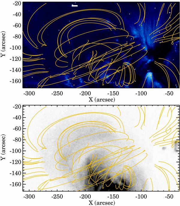
Figure 7. Top: TRACE 171 Å image of NOAA 10960, with over-plotted NLFF field lines. Bottom: Hinode/XRT SXR image, with over-plotted NLFF field lines. The NLFF field model is extrapolated from the Hinode/SOT-SP vector magnetogram that was taken on 2007 June 7 at 03:16 UT. TRACE 171 Å image was taken on the same day at 03:10 UT. Hinode/XRT SXR image was taken on the same day at 03:16 UT.
Download figure:
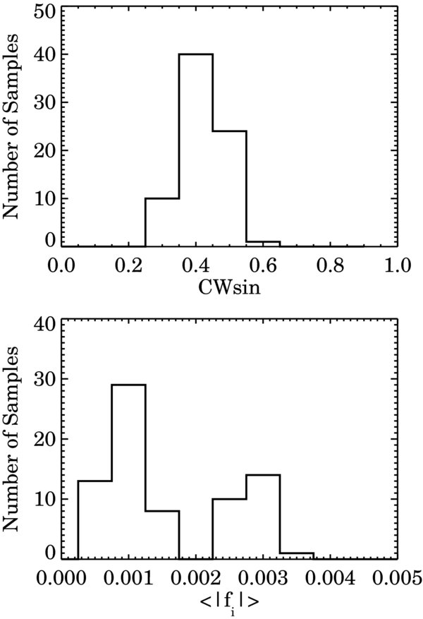
Standard image High-resolution imageSecond, we check how well the force-free and divergence-free conditions are satisfied over the computational domain by computing two metrics, the current-weighted sine metric, and 〈|fi|〉 metric (Wheatland et al. 2000), for each extrapolated field. Two metrics are defined as
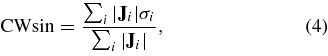
where
and
where Δx is the grid spacing. Clearly, CWsin and 〈|fi|〉 respectively reach a optimal value of zero for a perfect force-free and divergence-free field, with a smaller value indicating a more force-free and divergence-free state. Thereby, they have been used in many papers to evaluate the performance of NLFF fields (e.g., Metcalf et al. 2008; Schrijver et al. 2008; DeRosa et al. 2009). Figure 8 shows the distribution of CWsin and 〈|fi|〉 for our 75 samples. We note that the final state of the NLFF fields does contain residual forces and divergences.
Figure 8. Histograms of CWsin (top) and 〈|fi|〉 (bottom) metrics for the 75 samples.
Download figure:
Standard image High-resolution image
Third, we estimate the uncertainties in Efree caused by the image noise by employing a Monte Carlo method that was described by Guo et al. (2008), i.e., we add artificial noise to the vector magnetograms. The noise is in a normal distribution with the standard deviation of 5 G for Bz and 50 G for Bx and By, which is consistent with the sensitivity of Hinode/SOT-SP measurements. Then, we redo the 180° ambiguity resolution, preprocessing, and NLFF field extrapolation as described in Section 2. We repeat the same process 30 times, and find that the addition of noise leads to a standard deviation of Efree by ∼6%.
Additionally, it is worth mentioning that Wiegelmann et al. (2010) systematically test how strongly the instrumental effects (e.g., limited spatial resolution and spectral sampling) could influence the quality of NLFF fields. Since they used the same data set (Hinode/SOT-SP) and the data reduction methods as we do in this study, their result can be seen as a good object lesson for our reference. According to Wiegelmann et al. (2008, 2010), the combination of preprocessing and NLFF field extrapolation allows an estimation of free magnetic energy (in the low-β corona) from forced photospheric data with an error of a few percent.
Although the limitations of the NLFF field models in fully recovering the real coronal fields may undermine the value of this work, it is worthwhile experimenting with the correlation between free energy and flare productivity. Nevertheless, researchers should be aware of the lack of operational readiness of the NLFF field models and not over-interpret the results.
6. SUMMARY AND DISCUSSION
In this paper, we examine the magnitude scaling correlation between FIn−day and Efree based on the 75 samples, and also study the temporal variation of Efree with respect to the GOES SXR light curves for three active regions. The most important results are summarized as follows.
- 1.Efree is moderately to strongly correlated with FIn−day. The correlation confirms the physical link between magnetic energy and flare productivity of active regions. However, compared with two photospheric magnetic parameters Epe and Φ, Efree shows little improvement for flare predictability.
- 2.While the magnitude of Efree unambiguously differentiates between the flare-active and the flare-quiet regions, the temporal variation of Efree does not exhibit a clear and consistent pre-flare pattern.
One likely cause of the lack of satisfactory results is that the storage of Efree in magnetic fields is a necessary but not sufficient condition for the onset of solar flares. The trigger mechanism of flares is the determining factor of whether and when an active region will flare. Recently, there has been growing evidence relating emerging flux regions (EFRs) and magnetic helicity to the flare trigger mechanism. Magnetic helicity is a measure of magnetic topological complexity such as twists, kinks, and linkages of magnetic field lines (Berger & Field 1984). As suggested by a numerical simulation and supported by many observations, flares preferentially occur in the presence of a particular magnetic topology, which is prone to the annihilation of magnetic helicities with opposite signs between the newly EFR and the preexisting region (Kusano et al. 2003a, 2003b; Yokoyama et al. 2003; Wang et al. 2004; Jing et al. 2004). In addition, the monotonically increasing helicity over days prior to major flares has been found, which can be used as a warning sign of the flare onset (LaBonte et al. 2007; Park et al. 2008). We expect that a combination of Efree and magnetic helicity in future studies would carry extra weight in predicting flares.
Moreover, the energy release process involves a variety of dynamic phenomena such as flare heating, particle acceleration, and CME dynamics (Gibson et al. 2009). Consequently, the released Efree is converted and partitioned into the forms of thermal and non-thermal emissions and kinetic energy of CMEs. Considering that the SXR FI only quantifies a fraction of the released energy, i.e., the thermal part, we probably should not expect a very strong correlation between Efree and FIn−day.
Besides the concerns on flare trigger and energy release mechanisms, the NLFF field modeling from the photospheric boundary is subject to both observational limitations and intrinsic physical and/or mathematical problems. The observational limitations include the large uncertainties in transverse field measurements (Klimchuk & Canfield 1994), and 180° azimuthal ambiguity (Metcalf et al. 2006), etc. The physical/mathematical problems are related to the non-force-free nature of the photospheric boundary (Metcalf et al. 2008) and the difficulties of guaranteeing the existence and uniqueness of the NLFF field solutions (Rudenko & Myshyakov 2009). Although the use of high-quality magnetogram data and the advanced preprocessing and modeling algorithm improves the situation to some extent, the ability of the NLFF field model to reproduce the real coronal field, and Efree is seriously compromised (DeRosa et al. 2009). Moreover, the NLFF field is only a good approximation in the force-free domain (i.e., chromosphere and lower corona), not in the high-β photosphere and upper corona. Future improvements on magnetic field modeling may come from developing a self-consistent magnetohydrostatic (MHS) modeling (Wiegelmann & Neukirch 2006) and incorporating information on the coronal field topology as seen, for example, by TRACE and/or the twin Solar Terrestrial Relations Observatory (Wiegelmann et al. 2009).
The authors thank the anonymous referee for invaluable comments. The authors thank Dr. Aimee Norton and Dr. John Britanik for providing SOLIS magnetogram data. SOLIS data is produced cooperatively by NSF/NSO and NASA/LWS. The authors thank Hinode and team for their excellent data set. Hinode is a Japanese mission developed and launched by ISAS/JAXA, collaborating with NAOJ as a domestic partner, and NASA and STFC (UK) as international partners. Scientific operation of the Hinode mission is conducted by the Hinode science team organized at ISAS/JAXA. This team mainly consists of scientists from institutes in the partner countries. Support for the post-launch operation is provided by JAXA and NAOJ (Japan), STFC (UK), NASA, ESA, and NSC (Norway). J.J., Y.Y., and H.W. were supported by NSF under grant ATM 09-36665, ATM 07-16950, and NASA under grant NNX0-7AH78G and 8AQ90G. Y.X. was supported by NSF under grant ATM 08-39216. C.T. was supported by the Office of Sponsored Program, NJIT. T.W. was supported by DLR-grant 50 OC 0501.