


ABSTRACT
The black hole (BH)–bulge correlations have greatly influenced the last decade of efforts to understand galaxy evolution. Current knowledge of these correlations is limited predominantly to high BH masses (MBH≳108 M☉) that can be measured using direct stellar, gas, and maser kinematics. These objects, however, do not represent the demographics of more typical L < L* galaxies. This study transcends prior limitations to probe BHs that are an order of magnitude lower in mass, using BH mass measurements derived from the dynamics of H2O megamasers in circumnuclear disks. The masers trace the Keplerian rotation of circumnuclear molecular disks starting at radii of a few tenths of a pc from the central BH. Modeling of the rotation curves, presented by Kuo et al., yields BH masses with exquisite precision. We present stellar velocity dispersion measurements for a sample of nine megamaser disk galaxies based on long-slit observations using the B&C spectrograph on the Dupont telescope and the Dual Imaging Spectrograph on the 3.5 m telescope at Apache Point. We also perform bulge-to-disk decomposition of a subset of five of these galaxies with Sloan Digital Sky Survey imaging. The maser galaxies as a group fall below the MBH–σ* relation defined by elliptical galaxies. We show, now with very precise BH mass measurements, that the low-scatter power-law relation between MBH and σ* seen in elliptical galaxies is not universal. The elliptical galaxy MBH–σ* relation cannot be used to derive the BH mass function at low mass or the zero point for active BH masses. The processes (perhaps BH self-regulation or minor merging) that operate at higher mass have not effectively established an MBH–σ* relation in this low-mass regime.
1. DYNAMICAL BLACK HOLE MASSES
The past two decades have seen substantial improvements in our understanding of the demographics of nuclear supermassive black holes (BHs), predominantly driven by the availability of BH mass measurements for nearby galaxies from dynamical techniques. The advent of the Hubble Space Telescope (HST) has enabled a few dozen dynamical BH mass measurements, which reveal that supermassive BHs are ubiquitous components of bulge-dominated galaxy centers (e.g., Kormendy 2004). Furthermore, there appears to be a remarkably tight correlation between BH mass and bulge properties, including velocity dispersion (the MBH–σ* relation; Gebhardt et al. 2000; Ferrarese & Merritt 2000; Tremaine et al. 2002; Gültekin et al. 2009), luminosity (the MBH − Lbulge relation, e.g., Marconi & Hunt 2003), and mass (e.g., Häring & Rix 2004). The apparently tiny scatter in the MBH–σ* relation has led to a common view that the growth of BHs is intimately connected to the growth of the surrounding galaxy (see discussion in Ho 2004). In this paper, we explore the demographics of a new sample of dynamical BH masses measured using observations of circumnuclear masers (Kuo et al. 2010). Apart from our own Galactic Center, where individual stars are used as test particles to weigh the BH (e.g., Ghez et al. 2008; Gillessen et al. 2009), the most precise BH masses are derived using water megamaser spots in a Keplerian circumnuclear disk (e.g., Miyoshi et al. 1995). Such megamasers are very close to an ideal dynamical tracer of the central mass at the galaxy center, as they delineate a disk with a well-measured Keplerian rotation curve within fractions of a pc from the center. They are detectable when the disk is aligned within a few degrees of the line of sight. Masers detected in edge-on nuclear disks have characteristic triple-peaked spectral profiles, making the disk inclination angle well known in these cases (Lo 2005). BH mass measurements based on the Keplerian rotation curves of circumnuclear megamaser disks are not prone to the same systematic uncertainties as the dynamical methods based on optical observations. In the case of gas dynamical methods, it can be very difficult to determine the level of non-virial gas support (e.g., due to turbulence) but neglecting these extra sources of support can lead to significant bias in the final result (e.g., Barth et al. 2001). Stellar dynamical methods are sensitive to assumptions about galaxy anisotropy and radial variation in dark matter fraction that in general are not observationally well constrained (e.g., Gebhardt & Thomas 2009; van den Bosch & de Zeeuw 2010).
The cleanest and best-studied megamaser galaxy is the nearby Seyfert galaxy NGC 4258 (e.g., Nakai et al. 1993; Greenhill et al. 1995; Miyoshi et al. 1995; Herrnstein et al. 1996; for a complete literature review see Lo 2005). Observations of centripetal acceleration from the frequency change of the maser components at the systemic velocity of the system, combined with VLBA images of the megamaser disk, allow for the most precise extragalactic angular diameter distance measurement (Herrnstein et al. 1999). Other observations provide detailed constraints on the thickness, velocity structure, and toroidal magnetic field in an accretion disk (e.g., Modjaz et al. 2005; Herrnstein et al. 2005; Argon et al. 2007; Humphreys et al. 2008). For a long time it proved difficult to detect additional well-defined Keplerian megamaser disks, (e.g., Greenhill et al. 1997; Braatz et al. 1997; Kondratko et al. 2006b), but the situation has changed dramatically with the advent of the Robert C. Byrd Green Bank Telescope (GBT) of the NRAO.7 Thanks to the increased sensitivity of the GBT with a wide-band spectrometer, more megamaser candidates have been discovered (Braatz & Gugliucci 2008; Greenhill et al. 2009). Of the ∼130 extragalactic megamasers, approximately half were discovered with the GBT and ∼20 show evidence of originating in a disk.
The primary goal of ongoing megamaser searches is to find additional disk masers that can be used for angular diameter distance measurements in the Megamaser Cosmology Project (MCP; Reid et al. 2009; Braatz et al. 2010). With a sufficient number of angular diameter distances to galaxies in the Hubble flow, the MCP aims to determine a precise independent Hubble constant to a few percent accuracy (Reid et al. 2009; Braatz et al. 2010). An important outcome of the MCP is that the Keplerian megamaser disks also provide a precise measurement of the enclosed mass within a few tenths of a pc from the center of these spiral galaxies, dominated by a BH at the center, a valuable resource in its own right. The BH masses for seven maser galaxies are presented in Kuo et al. (2010). The present paper examines the demographics of the new megamaser galaxies, focusing on the shape and scatter of BH–bulge relations for these galaxies.
To date, the vast majority of dynamical BH masses have been obtained in massive elliptical and S0 galaxies (Figure 1). There are only five targets with BH mass measurements <107 M☉ (one of those being the Milky Way) and there are only 11 spiral galaxies with a Hubble type of Sa or later in the sample of 67 galaxies used in the most recent calibration of the MBH–σ* relation (Gültekin et al. 2009, Figure 1). The disproportionate representation of massive galaxies is easily understood. Local elliptical galaxies are relatively dust free, and the BHs are massive enough that we can resolve their gravitational spheres of influence at distances of tens of Mpc. Spiral galaxies tend to be dusty and star-forming, complicating dynamical measurements. Our knowledge of BH demographics at low masses is rudimentary, such that the shape and scatter in BH–bulge scaling relations as well as the BH occupation fraction in spiral galaxies remain uncertain (e.g., Greene & Ho 2007). The main focus of this work is to exploit the new sample of reliable BH masses afforded by the new maser studies to explore BH demographics for BHs with MBH ∼107 M☉ in spiral galaxies.

Figure 1. MBH–σ* relation as defined by nearby inactive galaxies from Gültekin et al. (2009), color coded by morphological type of the host galaxy. We distinguish between elliptical (red circles), S0 (green triangles), and spiral (blue squares) galaxies. The distribution of stellar velocity dispersion is shown in the black histogram in the top panel, also divided into the contribution of elliptical (red long-dashed lines), S0 (green short-dashed lines), and spiral (blue dot-dashed lines) galaxies. Similarly, the MBH distributions are shown in the right-hand panel. The histograms, as well as the black dashed lines, highlight the dearth of objects at σ*≲125 km s−1 and MBH≲107 M☉, the regime investigated by the current work.
Download figure:
Standard image High-resolution imageThe paper starts with a description of the sample (Section 2). We then describe the observations and data reduction (Section 3) and the spectroscopic (Section 4) and imaging (Section 5) analysis. In Section 6, we present the primary result of the paper, namely the location of the maser galaxies in the MBH–σ* plane, while in Section 7 the scalings between MBH and bulge luminosity/mass are briefly discussed. The impact of our results on our knowledge of BH demographics, particularly as probed with active galaxies, is discussed in Section 8, and we summarize and conclude in Section 9.
Throughout we assume the following cosmological parameters to calculate distances: H0 = 70 km s−1Mpc−1, Ωm = 0.30, and ΩΛ = 0.70.
2. THE SAMPLE AND THE BLACK HOLE MASSES
Over the years there have been a number of searches for megamaser galaxies (e.g., Braatz et al. 1997; Kondratko et al. 2006b; Braatz & Gugliucci 2008). By and large, the surveys have targeted known obscured active galaxies, with a detection rate of ∼5%. Once detected in a single-dish survey, megamasers that show disk characteristics, e.g., both systemic and high-velocity Doppler components, and that are bright enough, are subsequently imaged with very long baseline interferometry (VLBI) to map the positions and velocities of individual maser spots. The map determines whether a maser is in a clean dynamical system or has more complicated structures such as outflows (e.g., Kondratko et al. 2005).
In this paper, we present velocity dispersions both for the Kuo et al. sample and two other objects, NGC 3393 (Kondratko et al. 2008) and IC 2560 (Ishihara et al. 2001). In the latter case, while it is assumed that the systemic masers arise from the inner edge of the masing disk, without VLBI mapping the enclosed mass is uncertain by factors of a few. We expect better data will yield a concrete mass. The VLBI (and thus mass constraints) for the remaining seven objects are presented for the first time in Kuo et al. (2010). The details of the BH mass fitting are described in Kuo et al. but are reviewed here briefly for completeness. The BH masses are derived by fitting a Keplerian rotation curve to the positions and velocities of the maser spots (unlike NGC 1068 for instance; Lodato & Bertin 2003). The distance is fixed using an assumed value of H0 and the inclination of the maser disk is assumed to be 90°. All of the megamaser disks for which we have measured an inclination are within 6° of being perfectly edge-on, so the inclination contributes less than a 1% error to the measurement of the black hole mass. In NGC 4388, we could not measure a disk inclination, but even if the disk is 20° from edge-on, the contribution to the error in the BH mass would be only 12%, which is comparable to the BH mass error caused by the distance uncertainty (11%). Ongoing monitoring of the most promising targets will allow the measurement of accelerations in the systemic features. Joint modeling of MBH and distance for these targets will lead to a tighter constraint on each (e.g., Herrnstein et al. 1999).
It is interesting to note that the BH masses are strongly clustered around ∼107 M☉. We suspect that this is a simple consequence of picking random galaxies from the local active-galaxy mass function. Without accounting for incompleteness, the observed active mass function is strongly peaked at a mass ∼107 M☉ (e.g., Heckman et al. 2004). At higher mass, there are very few systems radiating at an appreciable fraction of their Eddington limit and we are woefully incomplete at lower mass (Greene & Ho 2007; Schulze & Wisotzki 2010). While we do not sample the full range of BH masses in the local Universe with this sample, our selection is unbiased with respect to bulge mass and velocity dispersion and thus does not invalidate our results.
The megamaser galaxies are found predominantly in early-to-mid-type spiral galaxies, ranging in Hubble type from S0 (e.g., NGC 1194) to Sb (e.g., NGC 4388). Table 1 includes the RC3 morphological types (de Vaucouleurs et al. 1991) and B-band luminosities and colors from Hyperleda (Paturel et al. 2003). As noted above, the parent sample consists predominantly of known active galaxies, ranging in distance from 18 to 150 Mpc. Only UGC 3789 did not have a documented active galactic nucleus (AGN) when the circumnuclear maser was discovered, although is it a narrow-line AGN. With the exception of NGC 4388, which has a weak broad Hα line (Ho et al. 1997), the active galaxies are classified as narrow-line (obscured) AGNs from the optical spectra. Furthermore, those with X-ray spectra have large column densities. Most are Compton thick (NH>1024 cm−2; Guainazzi et al. 2005; Madejski et al. 2006; Zhang et al. 2006; Kondratko et al. 2006a; Greenhill et al. 2008; Zhang et al. 2010). The only exceptions are NGC 4388, which has been observed to undergo large variations in column density over time scales of hours (Elvis et al. 2004), and NGC 6264, NGC 6323, and UGC 3789, which have not yet been observed in the X-rays. The attempted XMM-Newton observations of the former two were destroyed by flaring.
Table 1. Sample and Observations
| Galaxy | R.A. | Decl. | D | Hubble Type | MB | B − V | Instr. | Obs. Date | P.A. | texp |
|---|---|---|---|---|---|---|---|---|---|---|
| (1) | (2) | (3) | (4) | (5) | (6) | (7) | (8) | (9) | (10) | (11) |
| NGC 1194 | 03:03:49.1 | −01:06:13 | 52.0 | SA0+ | −20.3 | 1.03 | B&C | 2010-03-12 | 139 | 1500 |
| NGC 2273 | 06:50:08.6 | +60:50:45 | 26.0 | SB(r)a: | −20.2 | 0.94 | DIS | 2009-05-01 | 68 | 1500 |
| UGC 3789 | 07:19:30.9 | +59:21:18 | 50.0 | (R)SA(r)ab | −20.5 | ... | DIS | 2009-05-01 | 165 | 2700 |
| NGC 2960 | 09:40:36.4 | +03:34:37 | 71.0 | Sa? | −20.8 | ... | B&C | 2010-03-12 | 40,130 | 3600,3600 |
| IC 2560 | 10:16:18.7 | −33:33:50 | 41.8 | (R')SB(r)b | −21.3 | 0.97 | B&C | 2010-03-14 | 44,134 | 4800,4800 |
| NGC 3393 | 10:48:23.4 | −25:09:43 | 53.6 | (R')SB(rs) | −20.9 | 0.88 | B&C | 2010-03-12 | 158,68 | 5400,4800 |
| NGC 4388 | 12:25:46.7 | +12:39:44 | 19.0 | SA(s)b: | −21.9 | ... | B&C | 2010-03-13 | 91,1 | 3600,3600 |
| NGC 6264 | 16:57:16.1 | +27:50:59 | 136.0 | S? | −21.1 | ... | B&C | 2010-03-13 | 24,116 | 3000,3600 |
| NGC 6323 | 17:13:18.1 | +43:46:57 | 105.0 | Sab | ... | ... | DIS | 2010-03-13 | 176 | 2100 |
Notes. Column 1: name; Column 2: Right Ascension (HH:MM:SS; J2000); Column 3: Declination (DD:MM:SS; J2000); Column 4: distance (Mpc); Column 5: Hubble type from RC3 (de Vaucouleurs et al. 1991) as compiled in NED; Column 6: absolute B-band magnitude (mag) from Hyperleda; Column 7: B − V (mag); Column 8: instrument used for observations. The B&C spectrograph is on the Dupont telescope at Las Campanas, while DIS is on the 3.5 m telescope at Apache Point Observatory; Column 9: date of observation; Column 10: Position angle (°) East of North. When two slit positions were used, both P.A.s are listed; Column 11: total duration of spectroscopic exposure (sec). Two values correspond to major and minor axis exposure times, respectively.
Download table as: ASCIITypeset image
3. OBSERVATIONS AND DATA REDUCTION
The primary observations discussed here were obtained using the Dupont 2.5 m telescope at Las Campanas Observatory in the South, and the Apache Point Observatory (APO) 3.5m telescope in the North. In the Appendix, we describe an auxiliary data set that we use to cross-check our velocity dispersion measurements. At the Dupont telescope, we used the Boller & Chivens (B&C) spectrograph with the 600 lines mm−1 grating and the 2'' slit, which yielded an instrumental resolution of σr ∼ 120 km s−1 and a wavelength coverage of 3400–6600 Å, covering the 4000 Å break, the G band at 4304 Å, Hβ+[O iii]λλ4959, 5007, the Mg ibλλ5167, 5173, 5184 triplet, and (in most cases) Hα. We observed at two slit positions (Table 1) for the majority of the galaxies, both along the major and minor axis, at the lowest possible air mass to mitigate differential refraction. We observed the Northern targets with APO using the Dual Imaging Spectrograph (DIS), with a 1 5 slit, a 1200 lines mm−1 grating, a central wavelength of 4820 Å, a spectral range of 4250–5400 Å and a dispersion of σinstr ≈ 52 km s−1, as measured from the arc lines. These observations were performed at the galaxy major axis only. We also present one calcium triplet λλ8498, 8542, 8662 (CaT) measurement, based on a red setting with a central wavelength of 8540 Å (8000–9100 Å) and comparable instrumental resolution.
The reduction of both the DIS and B&C data proceeded in a similar fashion. Flat-fielding, bias-subtraction, and wavelength calibration were performed within IRAF.8 In the case of the B&C data, flux calibration and telluric correction was also performed within IRAF, using LTT 3218, LTT 3864, LTT 6248, Hilt 600, LTT 3218, Feige 56, and CD 32 as flux calibrator stars in order to match the air mass and time of observation. Flux calibration and telluric correction of the DIS data used IDL routines as described by Matheson et al. (2008). In this case, we used Feige 34 as the flux calibrator. In the Appendix, we compare the [O iii] luminosities between two independent data sets and demonstrate that our flux calibration is good to ∼30%.
The proper physical aperture used to calibrate the MBH–σ* relation remains a matter of debate (e.g., Ferrarese & Merritt 2000; Tremaine et al. 2002), and at present robust re measurements are only available for a small fraction of the maser sample. Thus, we have chosen to extract spectra with apertures ranging from the resolution limit of the observations (∼2'') to the signal-to-noise ratio (S/N) limit of the spectra (∼10''). Typically the S/N is optimized with apertures of ∼4''. The resulting dispersion in σ* values is included in the error budget, and is ≲10%.
4. STELLAR VELOCITY DISPERSIONS
We use direct-pixel fitting (e.g., Burbidge et al. 1961) to measure stellar velocity dispersions. The stellar templates are broadened and fitted in pixel rather than Fourier space. This method is computationally expensive relative to Fourier methods (e.g., Tonry & Davis 1979; Simkin 1974; Sargent et al. 1977; Bender 1990), but by no means prohibitive by modern standards. Direct pixel fitting provides many benefits over Fourier techniques (e.g., Rix & White 1992; van der Marel 1994; Kelson et al. 2000; Barth et al. 2002; Bernardi et al. 2003). For one thing, it is easier to incorporate noise arrays directly. Of particular importance to active galaxies, arbitrary regions of the spectrum (such as narrow emission lines) may be masked in a straightforward manner without introducing spurious signals into the final results.
The details of the code used here are described in Greene & Ho (2006a) and Ho et al. (2009). In short, each spectrum is modeled as the linear combination of template stars T(λ) that are shifted to zero velocity, broadened by a Gaussian, G(λ), with width σ and diluted by a constant [or power law if necessary; C(λ)]. Finally, the entire model is multiplied by a polynomial [P(λ); typically third order] to account for intrinsic spectral differences, reddening, and errors in flux calibration:

The nonlinear Levenberg–Marquardt algorithm, as implemented by mpfit in IDL (Markwardt 2009), is used to minimize χ2 in pixel space between the galaxy and the model. We have a library of template stars observed with the B&C spectrograph. For the fitting we use the following stars: HD 36634 (G6 III), HD 129505 (G8 IIII), HD 126571 (K0 III), HIP 70788 (K3 III), and HD 131903 (A9 V). For the APO observations, our spectral library is much more limited, and we have only one reliable velocity template star. Thus, we utilize a large library of high S/N, high-spectral resolution (∼26 km s−1) stellar templates from Valdes et al. (2004). Specifically, we use the following stars: HD 26574 (F2 II-III), HD 107950 (G6 III), HD 18322 (K1 III), and HD 131507 (K4 III). In order to translate the measured dispersion to the true dispersion, we first measure the instrumental dispersion of the DIS spectra using arc lines (52 km s−1), which yields a quadrature difference of (522–262)0.5 = 45 km s−1 between the DIS and Valdes spectra. We also measure the dispersion of the DIS velocity template using a Valdes star of the same spectral type and find 45 km s−1. The consistency of the two methods is reassuring. Thus, the final dispersion is simply σ* = (σ2meas − 452)0.5. Note that because we use stellar templates observed with an identical instrumental set-up, we need apply no corrections to the B&C spectra.
Given our spectral coverage, the most robust spectral features with high enough equivalent width (EW) for dispersion measurements are either the Mg ib triplet or the G band. We avoid the Ca H+K features because they are highly sensitive to spectral type, occur in a spectral region with a strong continuum discontinuity, and may be contaminated by interstellar absorption (see review in Greene & Ho 2006a). The Mg ib features are in many cases contaminated by emission from [Fe vii]λ5158 and [N i] λλ5198, 5200. Furthermore, differences in the α/Fe ratios between the template stars (from the solar neighborhood) and external galaxies will lead to systematic errors in σ* measurements from this region (Barth et al. 2002). For these reasons, we focus on the G-band region for the velocity dispersion measurements. We have multiple slit positions for most of the Dupont spectra. In Table 2, we present measurements for each slit position with the 4'' aperture, but we also present the weighted mean of the two, and use that value in all subsequent work. Example fits are shown in Figure 2 while the dispersions are presented in Table 2.

Figure 2. Example fits to four objects in the sample. Left: stellar velocity dispersion fits to two B&C spectra, using the best-fit weighted sum of an A9, G6, G8, K0, and K3 star. We plot the B&C spectra along the major axis (middle; thick histogram), the same along the minor axis (top; thin histogram), best-fit models (red solid), and residuals (bottom; thin histogram), while regions excluded from the fit are demarcated with gray bars. Flux density is normalized to the continuum. Right: spectra displayed as above, but we have only major axis spectra observed with DIS. Here, we used an F2, G6, K1, and K4 star.
Download figure:
Standard image High-resolution imageTable 2. Galaxy Properties
| Galaxy | log σ* | log σmaj | log σmin | r | Ar | Ag | B/T | g − r | ϒr | log Mbulge | log MBH | f1Gyr |
|---|---|---|---|---|---|---|---|---|---|---|---|---|
| (1) | (2) | (3) | (4) | (5) | (6) | (7) | (8) | (9) | (10) | (11) | (12) | (13) |
| NGC 1194 | 2.17 ± 0.07 | ... | ... | 14.0 ± 0.3 | 0.21 | 0.29 | 0.5 ± 0.2 | 0.7 ± 0.3 | 2.6 ± 1.6 | 10.3 ± 0.4 | 7.82 ± 0.05 | <0.05 |
| NGC 2273 | 2.16 ± 0.05 | ... | ... | ... | ... | ... | ... | ... | ... | ... | 6.88 ± 0.05 | ... |
| UGC 3789 | 2.03 ± 0.05 | ... | ... | ... | ... | ... | ... | ... | ... | ... | 7.05 ± 0.05 | ... |
| NGC 2960 | 2.22 ± 0.04 | 2.17 ± 0.04 | 2.26 ± 0.04 | 14.3 ± 0.1 | 0.12 | 0.17 | 0.4 ± 0.1 | 0.5 ± 0.1 | 2.0 ± 0.1 | 10.2 ± 0.1 | 7.05 ± 0.05 | 0.19 ± 0.13 |
| IC 2560 | 2.15 ± 0.03 | 2.13 ± 0.03 | 2.18 ± 0.03 | ... | ... | ... | ... | ... | ... | ... | ... | 0.20 ± 0.13 |
| NGC 3393 | 2.17 ± 0.03 | 2.15 ± 0.03 | 2.19 ± 0.03 | ... | ... | ... | ... | ... | ... | ... | 7.49 ± 0.12 | 0.02 ± 0.01 |
| NGC 4388 | 2.03 ± 0.03 | 2.02 ± 0.03 | 2.05 ± 0.03 | 12.0 ± 0.4 | 0.09 | 0.13 | 0.5 ± 0.2 | 0.4 ± 0.4 | 1.3 ± 0.1 | 9.79 ± 0.3 | 6.93 ± 0.05 | <0.05 |
| NGC 6264 | 2.20 ± 0.04 | 2.22 ± 0.04 | 2.06 ± 0.04 | 15.4 ± 0.2 | 0.18 | 0.25 | 0.5 ± 0.1 | 0.4 ± 0.2 | 1.4 ± 0.1 | 10.2 ± 0.1 | 7.45 ± 0.05 | 0.001 ± 0.001 |
| NGC 6323 | 2.20 ± 0.07 | ... | ... | 16.0 ± 0.1 | 0.05 | 0.07 | 0.2 ± 0.1 | 0.7 ± 0.1 | 2.8 ± 0.1 | 10.0 ± 0.1 | 6.96 ± 0.05 | ... |
Notes. Column 1: galaxy; Column 2: σ* within ∼4'' (km s−1); weighted average of two slit positions when available. Column 3: σ* within ∼4'' (km s−1) measured along the major axis; Column 4: σ* within ∼4'' (km s−1) measured along the minor axis, when available; Column 5: r−band bulge magnitude (mag), as measured from SDSS images using GALFIT; Column 6: galactic reddening (mag) in the r band; Column 7: galactic reddening (mag) in the g band. Column 8: bulge-to-total ratio in the r band; Column 9: g − r color (mag) measured from SDSS images, fixing the g-band model to that derived from r; Column 10: mass-to-light ratio (ϒ☉) of the bulge in the r band inferred from the g − r color using the relations presented in Bell et al. (2003). Note that the values are considerably lower than in elliptical galaxies; Column 11: bulge mass (M☉) as estimated from the r-band luminosity (Column 5) and the ϒr (Column 10); Column 12: black hole mass (M☉) as measured using megamaser spots that are in Keplerian rotation fractions of a pc from the black hole (Kuo et al. 2010); Column 13: fraction of light in a 1 Gyr population as estimated from fits to our spectra using Bruzual & Charlot (2003) stellar population models with an exponential decay time of τ = 1 Gyr. The spectra are fit with two components, one with an age of 1 Gyr, and the other with an old population of 10 Gyr. In all cases the 10 Gyr population dominates the light in the aperture.
Download table as: ASCIITypeset image
4.1. Literature Comparison
There are literature measurements available for a limited number of targets in our sample. Direct comparison can be tricky; the dispersions may be highly aperture dependent (e.g., Pizzella et al. 2004; Barbosa et al. 2006). Nevertheless, in general we find decent agreement with the literature values, as summarized in Figure 3. Two targets (NGC 2273, NGC 4388) appear in the recent atlas of stellar velocity dispersions measured for the Palomar spectroscopic survey of nearby galaxies (Ho et al. 1995), taken with a comparable 2'' × 4'' aperture (Ho et al. 2009). The two sets of observations agree within the uncertainties. For NGC 2273 we find 146 ± 17 km s−1 and Ho et al. present 149 ± 9 km s−1, while for NGC 4388 the values are 104 ± 10 km s−1 along the major axis and 92 ± 10 km s−1 along the minor axis. In the case of NGC 4388, note that our observation is only marginally spectrally resolved. However, our Sloan Digital Sky Survey (SDSS) measurement, presented in the Appendix, is 107 ± 11, giving us some confidence in this result. Other literature comparisons for these two targets are presented in Ho et al. (2009).
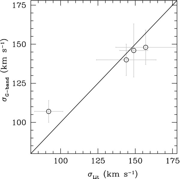
Figure 3. Comparison between our measured velocity dispersions and values from the literature (see Section 4.1 for the origin of each dispersion measurement). Note that we have not included the alternate dispersion for NGC 1194 (σ* =184 ± 18 km s−1).
Download figure:
Standard image High-resolution imageTwo other galaxies (NGC 3393 and IC 2560) were observed by Cid Fernandes et al. (2004) with a 15 × 082 slit. Again, the measurements agree within the quoted errors. In the case of IC 2560, we find 134 ± 12 km s−1 along the major axis compared to their 144 ± 20 km s−1, while for NGC 3393 we find 142 ± 16 km s−1 along the major axis and 156 ± 16 km s−1 along the minor axis, as compared to 157 ± 20 km s−1. NGC 3393 is also presented by Terlevich et al. (1990) measured within a 2'' extraction. They find 184 ± 18 km s−1, which is marginally consistent with our minor-axis measurement.
4.2. Emission Line Spectra and Bolometric Luminosities
One convenient by-product of our σ* measurement technique is a pure emission-line spectrum that has been corrected for underlying absorption lines (e.g., Hβ). Since the narrow emission lines (particularly [O iii]) represent one of the only methods for estimating bolometric luminosities for these obscured objects, we describe the measurements here. The fitting routines are described in Greene & Ho (2005) and Greene et al. (2009). Briefly, we fit the [O iii]λ4959, 5007 lines with sums of up to four Gaussians. The two lines are restricted to have identical shapes and the velocity difference and relative strengths are fixed to laboratory values (3.1 in the latter case). The Hβ line is fitted independently with the sum of two Gaussians (which is always completely sufficient given the typical signal-to-noise ratio, S/N, in this line). We also calculate the FWHM of the summation of all components in the [O iii] model. The velocity offsets between individual components are small compared to the total line width, so the FWHM is well defined. To bracket systematic uncertainties, we measure the line width in the spectra from the 4''and 10'' apertures and the error bar represents the difference in those two widths.
For the majority of the B&C spectra, as well as the DIS observation of NGC 6323, we also model the Hα+[N ii] complex. Ideally, we would use measurements of the [S ii] line width as a model to deblend Hα from [N ii]. (e.g., Ho et al. 1997; Greene & Ho 2005). However, in this case we simply describe each narrow line with the same combination of Gaussians, fix the relative strengths of the [N ii]λλ6548, 6583 lines to 1:2.96, and fix the relative wavelengths of all three lines to their laboratory values. In the case of NGC 4388, we further include a broad component fixed to have the same FWHM as reported by Ho et al. (1997), but we are not sensitive to the presence of weak broad lines in the other objects. We derive an intrinsic reddening correction for [O iii] using the Hβ and Hα fluxes when available, but do not apply it to the fluxes. All the line measurements are summarized in Table 3.
Table 3. AGN Properties
| Galaxy | fHβ | fHα | FWHM | log | log | log MBH | log /LEdd | log Lbol,x/LEdd | log /LEdd | ||
|---|---|---|---|---|---|---|---|---|---|---|---|
| (1) | (2) | (3) | (4) | (5) | (6) | (7) | (8) | (9) | (10) | (11) | (12) |
| NGC 1194 | 0.09 | ... | 30 | ... | 430 ± 43 | 39.9 | ... | 7.82 | −2.17 | ... | ... |
| NGC 2273 | 0.14 | 0.75 | 380 | 5 | 190 ± 19 | 40.5 | 40.1 | 6.88 | −1.64 | −2.85 | −2.06 |
| UGC 3789 | 0.08 | 0.47 | 700 | 3 | 200 ± 23 | 41.3 | ... | 7.05 | −0.82 | ... | ... |
| NGC 2960 | 0.09 | 0.31 | 50 | 1 | 700 ± 70 | 40.5 | ... | 7.05 | −1.65 | ... | ... |
| IC 2560 | 0.08 | 0.26 | 450 | 2 | 360 ± 36 | 41.0 | 41.1 | ... | ... | ... | ... |
| NGC 3393 | 0.10 | 0.24 | 630 | 1 | 460 ± 46 | 41.3 | ... | 7.49 | −0.80 | −1.47 | ... |
| NGC 4388 | 0.08 | 0.29 | 530 | 2 | 380 ± 38 | 40.4 | 41.6 | 6.93 | −1.76 | ... | 0.42 |
| NGC 6264 | 0.10 | ... | 80 | ... | 550 ± 55 | 41.3 | ... | 7.45 | −0.88 | ... | ... |
| NGC 6323 | 0.28 | ... | 20 | ... | 740 ± 255 | 40.4 | ... | 6.96 | −1.75 | ... | ... |
![$f_{ [{\rm O}\,{\hbox{\scriptsize{\sc{iii}}}}]}$](https://content.cld.iop.org/journals/0004-637X/721/1/26/revision1/apj362654ieqn1.gif)
![$r_{[{\rm O}\,{\hbox{\scriptsize{\sc{iii}}}}]}$](https://content.cld.iop.org/journals/0004-637X/721/1/26/revision1/apj362654ieqn2.gif)
![$_{\rm [O \,{\hbox{\scriptsize{\sc{iii}}}}]}$](https://content.cld.iop.org/journals/0004-637X/721/1/26/revision1/apj362654ieqn3.gif)
![$L_{\rm [O \,{\hbox{\scriptsize{\sc{iii}}}}]}$](https://content.cld.iop.org/journals/0004-637X/721/1/26/revision1/apj362654ieqn4.gif)
![$L_{\rm [O\, {\hbox{\scriptsize{\sc{iv}}}}]}$](https://content.cld.iop.org/journals/0004-637X/721/1/26/revision1/apj362654ieqn5.gif)
![$L_{\rm bol,[O \,{\hbox{\scriptsize{\sc{iii}}}}]}$](https://content.cld.iop.org/journals/0004-637X/721/1/26/revision1/apj362654ieqn6.gif)
![$L_{\rm bol,[O\, {\hbox{\scriptsize{\sc{iv}}}}]}$](https://content.cld.iop.org/journals/0004-637X/721/1/26/revision1/apj362654ieqn7.gif)
Notes. Column 1: galaxy name; Column 2: flux in Hβ normalized to flux in [O iii] (Column 4). Corrected for Galactic reddening only (see Table 2); Column (3): Hα flux normalized to [O iii] flux (Column 4); Corrected for Galactic reddening as above; Column (4): flux in [O iii] λ5007 line (10−15 erg s−1 cm−2). Corrected for Galactic reddening as above. Column (5): internal reddening correction to [O iii] as derived using the Balmer decrement (Columns 2, 3). We have not applied this correction to any emission-line measurements; Column (6): FWHM in the [O iii] line (km s−1) as measured within a 4'' aperture to match the σ* measurement, with the instrumental resolution subtracted in quadrature; Column (7): Luminosity (erg s−1) in the [O iii] line; Column (8): Luminosity in the [O iv]λ25.89μm line from Diamond-Stanic et al. 2009; Column (9): Black hole mass (M☉) as measured by Kuo et al. (2010) using megamaser spots. Repeated here for convenience; Column (10): Inferred Eddington ratio, with the bolometric luminosity (erg s−1) based on and the bolometric correction from Liu et al. 2009; Column (11): inferred Eddington ratio, with the bolometric luminosity (erg s−1) based on modeling of the Fe Kα line from Levenson et al. (2006); Column (12): Inferred Eddington ratio, with the bolometric luminosity (erg s−1) based on the measured (Column 8) and the bolometric correction of J. R. Rigby et al. (2010, in preparation).

![$L_{\rm [O\,{\mathsc iii}]}$](https://content.cld.iop.org/journals/0004-637X/721/1/26/revision1/apj362654ieqn9.gif)


![$L_{\rm [O\,{\mathsc iv}]}$](https://content.cld.iop.org/journals/0004-637X/721/1/26/revision1/apj362654ieqn12.gif)
Download table as: ASCIITypeset image
We are primarily interested in the [O iii] luminosities as an isotropic indicator of the AGN luminosity. Estimating robust bolometric luminosities in these objects is complicated since megamaser systems are found preferentially in obscured active galaxies (e.g., Braatz et al. 1997). Among the systems with circumnuclear disks, >75% are Compton thick (e.g., Zhang et al. 2006, 2010; Greenhill et al. 2008). Thus, there are only a few available luminosity diagnostics that are thought to be isotropic and immune from significant absorption. One is the strong and ubiquitous [O iii] line that has been used both to find AGNs and to determine their intrinsic luminosities (e.g., Kauffmann et al. 2003; Zakamska et al. 2003) although concerns about reddening remain (e.g., Mulchaey et al. 1994; Meléndez et al. 2008). The shape and EW of the Fe Kα line at 6.7 keV are also sensitive to the intrinsic luminosity and inclination of the obscuring material (e.g., Levenson et al. 2002). In a few cases, detailed modeling of the Fe Kα lines have been performed, which yields an independent estimate of the bolometric luminosities (Levenson et al. 2006). Finally, Diamond-Stanic et al. (2009) argue for the use of the [O iv] λ25.89μm emission line as a higher-fidelity tracer of AGN bolometric luminosity (see also Meléndez et al. 2008; Rigby et al. 2009).
Using the [O iii] bolometric correction presented in Liu et al. (2009), we derive bolometric luminosities for the entire sample using our measurements of L[OIII] (Table 3). Since this bolometric correction was derived without correction for internal reddening, we do not deredden either, but tabulate the proper correction for reference and comparison with the other indicators. The estimated Eddington ratios range from =10−2–0.16. Including internal reddening would change the values by 0.6 dex at most. There are only two objects with estimated bolometric luminosities from the Fe Kα line (excluding IC 2560 for the moment), also shown in Table 3. There are also three cases with [O iv] measurements in the literature; we have converted to bolometric luminosity using the calibration of J. R. Rigby et al. (2010, in preparation). As expected, Lbol([O iv]) tends to be higher than Lbol([O iii]), but the number of objects is too small to draw definite conclusions about the average magnitude of this effect, or how directly it is related to our internal reddening estimates.

4.3. Stellar Populations
The presence or absence of young stellar populations in the bulge regions of these galaxies provide important clues as to their growth and evolution (Section 5.3). The spectra provide useful constraints on stellar ages, although the modeling is complicated by the narrow emission lines that litter the spectrum. We do not perform full stellar population synthesis modeling. Instead, we take a few representative sets of Bruzual & Charlot (2003) models and perform a least-squares fit to the galaxy continua, fixing the stellar velocity dispersion to that derived above. We adopt the Padova isochrones (Marigo & Girardi 2007) and a Chabrier (2003) initial mass function. We take both single-age stellar population models and exponentially decaying models with a decay time τ = 1 Gyr. For simplicity, we use two models with ages of one and 10 Gyr respectively, although we experiment with models having ages of 0.5 and 5 Gyr and also one-half of solar metallicity. We adopt a single reddening screen for each galaxy, using the reddening law of Calzetti et al. (2000). See example fits in Figure 4. The fraction of light in young stars is tabulated in Table 2.

Figure 4. Three examples of fits to the entire spectral range using high-resolution Bruzual & Charlot (2003) models (see Section 4.3). We plot the original spectra (thick black histogram), the best-fit model with σ* fixed (red solid) and the residuals (thin black histogram). Flux density is arbitrarily normalized and masked regions are indicated with gray bars.
Download figure:
Standard image High-resolution imageOf the six galaxies for which our spectra include the 4000 Å break, we see that only two show evidence for a significant contribution from intermediate-age populations (NGC 2960 and IC 2560). NGC 3393 and NGC 6264 may have a very minor young component, but presumably higher spatial resolution would be needed to isolate it. We can compare these results with the more detailed stellar population fits of Cid Fernandes et al. (2004), whose sample also includes IC 2560, NGC 4388, and NGC 3393. In NGC 3393, we both agree that the stellar populations are old; Cid Fernandes et al. find that 4% of the luminosity in this source come from stars with an age <25 Myr. They find a substantial 33% contribution from young stars in IC 2560, consistent with our findings. The only ambiguous case is NGC 4388. They find that 13% of the luminosity comes from this young component, while we do not find compelling evidence for a young component. In fact, NGC 4388 is quite difficult to model, both because it is extincted and because the emission lines have very high EWs.
Those galaxies (NGC 2273, UGC 3789, and NGC 6323) that we observed with APO do not have the blue coverage needed to constrain the stellar populations. In the case of NGC 2273, young stars associated with an inner ring are wel documented (Gu et al. 2003). Unfortunately, we do not have much information for the other two. The bulge color of NGC 6323, g − r = 0.7 (see below), is typical for an early-type spiral galaxy (Fukugita et al. 1995), suggesting that either there is not much star formation and/or that there is a considerable quantity of dust. Overall, we find evidence for ongoing or recent star formation in roughly half of the sample.
4.4. Uncertainties: Aperture Effects, Rotation, and Bars
As discussed briefly in Section 2, the velocity dispersion profiles of late-type spirals can be complicated by kinematically cold, disk-like components as well as bars or other non-axisymmetries. As a result, it is impossible to pick a single, well-motivated aperture size, and the long-slit data presented here are not deep enough to derive robust rotation curves. We can say that the measured dispersions do not change by more than 10% over the range of radii we probe, and this spread in values is included in the error budget. Robust re measurements are needed to define the optimal radius of extraction for each galaxy. Along similar lines, it is possible that the slit orientation relative to that of the bar might impact σ* (e.g., Kormendy 1983; Emsellem et al. 2001). However, for the objects with both minor and major axis spectra, we see at most a 40% difference in the two measurements. Ideally, we would like to obtain integral-field spectroscopy for the objects to settle this ambiguity.
An additional concern is that differing stellar populations and metallicities lead to bias due to template mismatch. While our code includes a mix of spectral types, subtle systematics from region to region remain (see an example in Ho et al. 2009). When we calculate errors in σ*, we include the differences between the nominal dispersions and those measured from the 5100–5400 Å region [excluding the Mg ib lines themselves since variations in α/Fe tend to bias the dispersion measurements high (e.g., Barth et al. 2002)].
5. PHOTOMETRIC DECOMPOSITION
Often, spiral galaxies contain bars, ovals, rings, dust lanes, nuclear spirals, and nuclear star clusters in their centers (e.g., Carollo et al. 1997; Böker et al. 2002; Martini et al. 2003). Furthermore, in galaxies with young stellar populations, the mass-to-light ratio (ϒ) may vary significantly both within a given galaxy and from object to object. To properly decompose such light profiles requires both deep imaging on large scales to quantify the disk component and high resolution nuclear imaging, ideally in a red band, to reveal the complex nuclear morphology.
We first tried to perform detailed profile decompositions using Two-Micron All-Sky Survey (2MASS) images (Skrutskie et al. 2006). As shown in Figure 5, these images are too shallow to detect large-scale disks and rings. Furthermore, the resolution (2–3'') is insufficient to uncover nuclear features. A combination of K-band observations with HST and from the ground is needed to fully model the entire galaxy. As an initial exploration we have settled on a compromise. There are five galaxies that fall within the SDSS footprint. We have performed two-dimensional image decomposition on the gr images of these five galaxies, which allows us to measure a magnitude and a color for their bulge components. We then use the relations of Bell et al. (2003) to convert the g − r color into ϒr and thereby stellar mass.

Figure 5. SDSS r-band images (left) and radial profiles (right) for the galaxies NGC 1194 (top) and NGC 6264 (bottom). A scale of 10'' is shown. The radial profiles show the K band (open circles) and SDSS r band (filled circles) isophotes, in order to demonstrate that the optical data are both deeper and have higher resolution.
Download figure:
Standard image High-resolution image5.1. GALFIT
We perform image decomposition in two dimensions using the program GALFIT (Peng et al. 2002). Two-dimensional fitting allows flexibility in the ellipticities and position angles of different components that can help break degeneracies in fitting multi-component galaxies (e.g., Andredakis et al. 1995; Wadadekar et al. 1999) as reviewed in detail in Peng et al. (2010).
GALFIT and related programs create model galaxies as the sum of ellipsoids with parametrized surface brightness profiles that are convolved with the point-spread function (PSF) of the image and then compared with the data. Best-fit parameters are those that minimize the differences between data and model. In general, we model the galaxies with Sérsic (1968) functions:

where re is the effective (half-light) radius, Ie is the intensity at re, n is the Sérsic index, and bn is chosen such that

An exponential disk has n = 1 while n = 4 corresponds to the well-known de Vaucouleurs (1948) profile. We adopt the PSF models provided by the SDSS,9 and note that our analysis is not very sensitive to the detailed PSF shape. Unlike typical two-dimensional modeling, GALFIT now incorporates coordinate rotations and Fourier modes (departures from axisymmetric modeling) that are particularly useful in handling dust-lanes, bars, and spiral structure (Peng et al. 2010).
As described above, in addition to the structural measurements we also need color information to estimate the stellar masses of the galaxies. We first fit the r-band images to extract structural information and then apply the same model to the g-band images, allowing only the total flux to vary for each component. In Figure 6 we show the fits to the r-band images. We caution that the measurements are preliminary in the absence of high-resolution imaging. Therefore, we present only the "bulge" luminosities and colors, and reserve more detailed discussion of the galaxy structure (e.g., Sérsic index) to future work. For the moment, we simply note that the bulge colors provide an additional crude handle on the stellar populations in these galaxies (Table 2). In the case of NGC 1194 and NGC 6323, the g − r color is typical of Sa galaxies (Coleman et al. 1980; Fukugita et al. 1995), NGC 2960 has the color of an Sbc galaxy, and NGC 4388 and NGC 6264 are the bluest, with colors typical of Scd galaxies.

Figure 6. Photometric fits to all objects with SDSS images. We show the r band image (left) with a scale bar of 20'', the best-fit GALFIT model (middle), and the residuals (right), as well as radial profiles for the data (black circles), the total model (solid black line), any bulge (red solid line), disk (blue solid line), bar (green solid line), or outer disk (magenta solid line). Residuals are shown beneath in solid squares. Note that dust-lanes and spiral arms can introduce non-monotonic behavior in the radial profiles.
Download figure:
Standard image High-resolution image5.2. Uncertainties In Decomposition
Clearly, errors in the PSF shape and sky level add scatter to the photometric decompositions. We expect that these uncertainties are <0.1 mag. Therefore, we are dominated by systematic errors. More specifically, because of prominent dust lanes in many galaxies, combined with the limited spatial resolution of the SDSS, we do not have a strong constraint on the Sérsic index of the bulge, which in turn contributes large errors to the effective radii as well as in the ratio of bulge-to-total (B/T) luminosity.
Currently, our error bars represent the spread in derived luminosities resulting from a range of different models, which give some indication of the uncertainties due to model assumptions (e.g., Peng et al. 2010). After running these models, we report the one with the lowest value of reduced χ2 and assign parameter uncertainties based on the spread across the models. Let us take as an example the galaxy NGC 1194. In this case we have fit a model with the bulge Sérsic index fixed to n = 4 and the disk fixed to n = 1. As the next level of complexity we have allowed each component to vary freely, yielding n = 3.9 for the bulge and n = 2.2 for the "disk." Finally, we have run two models with different parameterizations of the dust lane that have n ≈ 2.7, n ≈ 1.5 for the bulge and disk respectively. In all cases, the fits would be deemed acceptable, but using a range of models allows us to quantify the dependence of the bulge parameters on our model assumptions. In this case, the resulting bulge magnitude varies by ∼0.5 mag between the model with n = 4 and those including dust. These systematic uncertainties exceed by far those resulting from sky and PSF uncertainties, and are the ones we report here.
5.3. Bulge Classification: Classical or Pseudobulge
In this subsection we discuss the morphological properties of the maser sample. In particular, we address the bulge morphology. First consider NGC 1194 (Figure 5(a)). This galaxy has a massive bulge component and is classified as an S0. Both in the radial profile and the image, it is clear that the bulge in NGC 1194 has smooth isophotes and a large ratio of B/T luminosities. Much more typical of the megamaser disk galaxies is NGC 6264, which has a strong bar (Figure 5(b)). Other barred galaxies include NGC 2273, NGC 3393, NGC 4388, and IC 2560. Roughly speaking, the bar fraction in the maser sample is consistent with the ∼60% seen in the spiral galaxy population (e.g., Eskridge et al. 2000; Menéndez-Delmestre et al. 2007).
Finally, we examine NGC 2273 (Figure 7), also a barred spiral galaxy. In addition, NGC 2273 contains two outer rings and a centrally concentrated bulge component (Erwin & Sparke 2003). Zooming in with HST/WFPC2 and NICMOS reveals that the galaxy center consists of an inner ring surrounding a nuclear spiral (e.g., Mulchaey et al. 1997; Erwin & Sparke 2003). This spiral component is very different in shape, kinematics and stellar populations from a classical bulge. The latter is understood to be a dynamically hot stellar component with an old stellar population, effectively an elliptical galaxy with a surrounding disk (see discussion in Kormendy & Kennicutt 2004). In contrast, the center of NGC 2273 is a disk with ongoing star formation fueled by a reservoir of molecular gas (e.g., Petitpas & Wilson 2002) that is likely fed by the larger-scale bar. Furthermore, there is a distinct drop in σ* within the inner 5'' where the kinematics are dominated by rotation, presumably because the young bright stars trace the motion of the gas in which they formed (Barbosa et al. 2006; Falcón-Barroso et al. 2006).

Figure 7. Three images of NGC 2273 at progressively smaller scales. The large-scale R-band images are from WIYN and were kindly provided by P. Erwin (Erwin & Sparke 2003; left, middle), while the nuclear spiral is a NICMOS/F160W image. Finally, we show the radial profiles for the NICMOS (blue open circles; top), WFPC2/F606W (red filled circles), and R-band (crosses) images.
Download figure:
Standard image High-resolution imageIt has been clear for a long time that the "bulges" of spiral galaxies are often disk-like. The first clues were kinematic, with some bulge-like components displaying very high ratios of rotational velocity to velocity dispersion (e.g., Binney 1978; Kormendy & Illingworth 1982; Kormendy 1993). HST imaging reveals disk-like and flattened central isophotes (e.g., Fathi & Peletier 2003; Fisher & Drory 2008; Andredakis & Sanders 1994; Courteau et al. 1996; MacArthur et al. 2003), bars, ovals, nuclear spirals, and rings in many bulge-like components (e.g., Carollo et al. 1997; Martini et al. 2003) as well as ongoing star formation (Fisher et al. 2009). To distinguish these systems from "classical" bulges, they are referred to as "pseudobulges." It is thought that secular, internal processes (e.g., bars or spiral arms) are responsible for building pseudobulge mass, in contrast to the rapid merging processes, i.e., violent relaxation, thought to build elliptical galaxies and classical bulges. The literature is reviewed in detail in Kormendy & Kennicutt (2004). Throughout, we will use the term "bulge" to refer to any luminous, centrally concentrated galaxy center, where classical bulges are of the elliptical type and pseudobulges are essentially disks.
Different authors use different (overlapping) criteria to identify pseudobulges. Fisher & Drory (2008) start with a sample of morphologically selected pseudobulges, meaning that a nuclear bar, spiral, or ring is detected within the bulge region (see also Kormendy & Kennicutt 2004). They show that the distribution of Sérsic indices in local bulges is bimodal, and suggest that pseudobulges are galaxies with n < 2 (for a definition of the Sérsic index, see Section 5.1). These authors also show that the average B/T of pseudobulges (0.16) is lower than that of classical bulges (0.4) with a large spread. Gadotti (2009), on the other hand, advocates use of the Kormendy (1977) relation as a discriminator, since pseudobulges tend to have lower central surface brightnesses at a fixed radius (see also Carollo 1999; Fisher & Drory 2008). Finally, while classical bulges are typified by old stellar populations, pseudobulges tend to have ongoing star formation (e.g., Kormendy & Kennicutt 2004; Drory & Fisher 2007; Fisher et al. 2009; Gadotti 2009). Since deriving robust velocity measurements is beyond the scope of this paper, and in the absence of more robust structural information, we rely on morphology and stellar population properties at the present time.
The nearest, well-studied targets in our sample (NGC 4388, and NGC 2273) probably contain pseudobulges. In the case of NGC 2273, this classification is based on both the young stellar populations and the rings and nuclear disk. NGC 4388 is less certain, but there is clear evidence for recent star formation and dust. We suspect that NGC 6264 contains a pseudobulge, given its morphological similarities with NGC 2273 (namely the outer ring and inner bar) and the evidence for young stars. The same goes for NGC 3393 and IC 2560, which each contain an outer ring, a bar, and an inner ring. On the other hand, NGC 1194, with both evolved stellar populations and a large bulge, probably contains a classical bulge. NGC 2960 has some of the clearest evidence for ongoing star formation, and so we tentatively put it into the pseudobulge category. Finally, we remain agnostic about NGC 6323, which is one of the most distant targets. Thus, of the nine targets we consider, at least seven likely contain pseudobulges.
6. SCALING BETWEEN MBH AND σ*
In Figure 8, we present the location of the megamaser galaxies in the MBH–σ* plane. The maser galaxies do not follow the extrapolation of the MBH–σ* relation defined by the elliptical galaxies. Instead, they scatter towards smaller BH masses at a given velocity dispersion. Quantitatively, taking ΔMBH ≡ log(MBH) − log[M(σ*)], where log[M(σ*)] is the expected MBH given σ*, we find 〈ΔMBH〉 = 0.24 ± 0.10 dex. There are many hints in the literature that the MBH–σ* relation does not extend to low-mass and late-type galaxies in a straightforward manner (e.g., Hu 2008; Greene et al. 2008; Gadotti & Kauffmann 2009). However, the precision BH masses afforded by the maser galaxies make a much stronger case. The MBH–σ* relation is not universal. Neither the shape nor the scatter of the elliptical galaxy MBH–σ* relation provides a good description of the maser galaxies in this plane.

Figure 8. Relation between BH mass and bulge velocity dispersion for the maser galaxies presented here (open circles) and those from the literature (gray stars). IC 2560 is indicated with a cross and the BH mass error bar is heuristic only. For reference, we show the MBH–σ* relation of elliptical galaxies from Gültekin et al. (2009, red dashed line). The maser galaxies trace a population of low-mass systems whose BHs lie below the MBH–σ* relation defined by elliptical galaxies. The largest outlier galaxies are (from highest to lowest MBH) NGC 2960, NGC 6323, and NGC 2273.
Download figure:
Standard image High-resolution imageWe now add the maser galaxies to the larger sample of local galaxies with dynamical BH masses to show that indeed a single, low-scatter power-law does not provide an adequate description of all galaxies in the MBH–σ* plane. For convenience and to facilitate comparison with previous work, we assume a power law for all fits, although that form may not provide the best description of the sample as a whole.
6.1. Sub-samples
We fit not only the full sample, but also divide the galaxies by morphological type. For ease of comparison, we adopt the divisions of Gültekin et al. (2009). In essence, the galaxies are divided into two primary morphological bins: elliptical and spiral galaxies. For completeness we perform fits assuming that S0 galaxies belong to each subgroup. We adopt nomenclature from Gültekin et al.. "Elliptical" refers only to the elliptical galaxies, while "early-type" refers to elliptical and S0 galaxies. "Late-type" galaxies are spiral galaxies excluding S0s while "nonelliptical" includes all spiral galaxies (S0 and later). All fits are shown in Table 4 and Figure 9.

Figure 9. Relation between BH mass and bulge velocity dispersion, including not only the maser sample (open circles) but also the sample from Gültekin et al. (2009). Each panel shows fits to a different sub-sample (see also Section 6.1). In each panel, literature maser galaxies are highlighted with open gray stars. IC 2560 is indicated with a cross and the BH mass error bar is heuristic only. For reference, the MBH–σ* relation of the elliptical galaxy sample (red dashed line) is shown in all panels. Top left: this panel includes all sub-samples and all fits, as follows. From Gültekin et al. we show the elliptical (filled red circles), S0 (green triangles), and spiral galaxies (blue squares). All of the fits are shown as well, including the best fit to the entire sample (thick black solid), the sample of Gültekin et al. (2009, thin black solid), the elliptical (red long-dashed) and non-elliptical (green dot-dashed) subsamples, and to the early (E/S0; magenta long dot-dashed) and late-type (blue short dashed) sub-samples. For the purpose of clarity we have omitted upper limits from the figures although they are included in the fits (see Section 6). Top right: here we plot the "nonelliptical" sample, consisting of S0 (green triangles) and later-type spiral (blue squares) galaxies. The original Gültekin et al. fit to the nonelliptical galaxies (thin green line) and our fit including the maser galaxies (green dot-dashed line) are shown. Bottom left: the "late-type" spiral galaxies alone (excluding the S0 galaxies; blue squares). Best fits to the sample excluding (thin blue solid) and including (blue short-dashed) the maser galaxies are shown. Bottom right: the "pseudobulge" subsample of the nonelliptical sample is highlighted here with purple asterisks. Note that both S0 and later-type spiral galaxies are included, as well as the majority of the maser galaxies. Fits excluding (thin purple solid) and including (purple short-long dashed) the maser galaxies are shown. Furthermore, we have performed a second fit (Pseudo2) excluding NGC 3245 and NGC 4342, since they have conflicting morphological designations in the literature. The two galaxies are highlighted with large black triangles, and the alternate fit is shown (dotted purple line).
Download figure:
Standard image High-resolution imageTable 4. Fits
| Sample | Nm | Nu | α | β |  |
|---|---|---|---|---|---|
| (1) | (2) | (3) | (4) | (5) | (6) |
| G09 | 49 | 18 | 8.13 ± 0.07 | 4.31 ± 0.38 | 0.43 ± 0.05 |
| G09+M | 58 | 18 | 8.09 ± 0.07 | 4.41 ± 0.37 | 0.44 ± 0.05 |
| Elliptical | 25 | 2 | 8.23 ± 0.08 | 4.05 ± 0.40 | 0.30 ± 0.05 |
| NE+M | 32 | 16 | 7.96 ± 0.13 | 3.93 | 0.48 ± 0.06 |
| NE+M | 32 | 16 | 7.95 ± 0.13 | 3.91 ± 0.72 | 0.48 ± 0.06 |
| Early | 38 | 6 | 8.22 ± 0.07 | 3.93 ± 0.37 | 0.34 ± 0.05 |
| Late+M | 19 | 12 | 7.85 ± 0.29 | 3.93 | 0.47 ± 0.08 |
| Late+M | 19 | 12 | 7.79 ± 0.22 | 3.54 ± 1.19 | 0.47 ± 0.07 |
| Pseudo+M | 19 | 2 | 7.84 ± 0.10 | 3.93 | 0.33 ± 0.06 |
| Pseudo+M | 19 | 2 | 7.86 ± 0.15 | 4.05 ± 0.86 | 0.33 ± 0.06 |
| Pseudo2+M | 14 | 2 | 7.79 ± 0.09 | 3.93 | 0.26 ± 0.05 |
| Pseudo2+M | 14 | 2 | 7.61 ± 0.14 | 2.77 ± 0.77 | 0.23 ± 0.05 |
Notes. Column 1: fitted Subset. G09 = Gultekin et al. 2009; NE = Nonelliptical galaxies; Pseudo = Pseudobulges; Pseudo2 = Pseudobulge sample from G09 excluding NGC 3245 and NGC 4342; M = Megamaser galaxies from this work; Column 2: number of detections included in the fit; Column 3: number of upper limits included in the fit; Column 4: best-fit intercept; Column 5: best-fit slope. In cases with no error bars the slope was held fixed; Column 6: best-fit intrinsic scatter.
Download table as: ASCIITypeset image
In addition to these two divisions, we also consider pseudobulges by themselves. Early work suggested that pseudobulges (see Section 5.3) obey the MBH–σ* relation of classical bulges based on a very small sample of galaxies (Kormendy & Gebhardt 2001). Further study, based on larger samples, has pointed to differences both in the slope and scatter of BH–bulge relations in pseudobulges (Hu 2008; Greene et al. 2008; Graham & Li 2009; Gültekin et al. 2009; Gadotti & Kauffmann 2009), but the results are not conclusive, predominantly because the available number of dynamical BH masses in pseudobulges is so small. The maser sample mitigates this problem. As a fiducial sample, we adopt the pseudobulges tabulated by Gültekin et al. However, both NGC 3245 and NGC 4342 were classified as classical bulges by Fisher & Drory (2008) and Kormendy (2001) respectively. Thus, we have performed a second fit (Pseudo2) excluding these two galaxies. While the slopes differ between the two fits (although not significantly), the intrinsic scatter does not change.
6.2. The Fitting
To facilitate direct comparison, we adopt the fitting procedure of Gültekin et al.. As is commonly done, we fit the relation: log (MBH/M☉) =β + α log(σ*/200 km s-1). We use a generalized maximum likelihood analysis that is designed to incorporate intrinsic scatter in a natural manner. For simplicity, we assume a Gaussian distribution in both the measurement errors and the intrinsic scatter (directly investigated by Gültekin et al.). For a set of observed points (Mi, σ*,i), we maximize the total likelihood:

In the presence of measurement errors, if the likelihood of measuring a mass Mobs for a true mass M is Qi(Mobs|M)dMobs, then for a given observation the likelihood is:

We assume both Q and P to have a log-normal form. Upper limits are included, where the mass is taken to be below the upper limit with a Gaussian probability given by the measurement uncertainty (see details in Appendix A of Gültekin et al.). Their inclusion does not change the fits significantly.
Since errors in the independent variable are not naturally included, we run 2000 Monte Carlo simulations for each fit in which the dispersion values are drawn from a Gaussian distribution around the measured value, assuming symmetrical errors in the logarithm. The reported error is a quadrature sum of the error from the fit and the width of the final distribution of fitted values from the Monte Carlo runs. As a sanity check, we also employ a χ2 fitting technique adapted from Tremaine et al. (2002). In this formalism, intrinsic scatter is included as an additional term such that the final reduced χ2 =1. While we only present results from the maximum likelihood treatment, we note that the fits are consistent between the two methods in all cases.
The formal fitting quantifies the visual impression of Figure 8. At low BH mass (MBH ≲107 M☉), galaxies begin to deviate significantly from the MBH–σ* relation of elliptical galaxies. The zero point is lower by 0.4 ± 0.2 dex and the scatter is larger by 0.2 ± 0.1 dex. It is worth noting that, in agreement with Gültekin et al., the fits to the pseudobulge galaxies are in no way distinguishable from fits to either the late-type or nonelliptical sub-samples. Our data demonstrate that the power-law relationship between MBH and σ* is not universal. Specifically, we find a population of BHs that apparently have not fully grown to the present day MBH–σ* relation of elliptical galaxies.
6.3. Potential Caveats
Our measurement techniques may not yield σ* values that are directly comparable with those in elliptical galaxies. There is firstly the question of whether we are contaminated by disk light. From the SDSS imaging, it is quite clear that the bulge completely dominates the light within 5''. As an additional sanity check, in Figure 10 awe look for correlations between the galaxy axial ratio (as proxy for the inclination) and deviations from the MBH–σ* relation, ΔMBH. There is no compelling evidence for a correlation between the two (Kendall's tau value of τ = −0.2 with a probability P = 0.7 that no correlation is present), suggesting that our σ* measurements are not strongly biased by rotation in the central regions.

Figure 10. (a) Large-scale disk axial ratio vs. deviations from MBH–σ* relation; ΔMBH≡log(MBH) − log[M(σ*)]. There is no clear correlation between the two, suggesting that our σ* measurements are not strongly biased by rotation in the central region. (b) We investigate a possible correlation between the Eddington ratio and ΔMBH. Again, we see no evidence for a significant correlation between the two, suggesting that deviations from the MBH–σ* relation are not driven by ongoing BH growth.

Download figure:
Standard image High-resolution imageWe still worry about aperture biases in our σ* measurements, because we do not fully sample the radial behavior of σ*. We have measured σ* within apertures ranging from 2'' to 10'', and the values only vary by <10% within this range. To reiterate, we are not reporting σ* within re at this time because we do not wish to fold the (large) uncertainties in the structural measurements into our dispersion measurements. In any case, the radial variations in σ* are insignificant on the scales we can currently measure. On the other hand, as NGC 2273 demonstrates, two-dimensional σ* profiles with higher spatial resolution may well reveal a decline in σ* within some galaxy centers.
Of course, there is the much more serious concern that these galaxies do contain small classical bulges. The recent paper by Nowak et al. (2010) presents direct evidence that isolating the classical bulge component in composite systems can bring later-type galaxies in line with the local elliptical galaxy MBH–σ* relation. We hope to investigate this concern directly in future work.
7. THE RELATION BETWEEN BH MASS AND BULGE MASS
Using the sub-sample of galaxies with SDSS data, we are able to investigate the correlation between MBH and Mbulge. We first show the MBH − Lbulge relation in Figure 11(a), along with the best-fit relation from Gültekin et al. (2009). The V−band luminosities are calculated from the r-band magnitudes and g − r colors, using a grid of average galaxy colors derived from the Coleman et al. (1980) templates. We caution that the sample is still small. Furthermore, we are only spatially resolving the inner ∼500 pc of these galaxies, while the nuclear spiral in NGC 2273 is <300 pc. At the same time, dust extinction is clearly significant in all of these systems, and while GALFIT now includes dust lanes, the uncertainties are substantial (e.g., B/T can vary by nearly a factor of two depending on our treatment).

Figure 11. (a) Relation between BH mass and bulge luminosity (large open circles) and between BH mass and total galaxy luminosity (small open circles) for the megamaser galaxies with SDSS observations. Bulge luminosities are derived by detailed image decomposition of SDSS r-band images using GALFIT (see Section 5, Figure 7), while the conversion to V-band luminosity is calculated as a function of g − r color using the Coleman et al. (1980) galaxy templates. The solid line shows the relation of Gültekin et al. (2009), while the small gray points are the objects from their sample in order to demonstrate the scatter typical in the inactive local samples. The low-mass galaxy anchoring the fit to the galaxies from Gültekin et al. is M32. Note that Gültekin et al. fit only E/S0 galaxies. Filled black circles are AGNs with reverberation-mapping as presented in Bennert et al. (2010) here plotted against total galaxy luminosity, while the squares are local AGNs with reverberation mapping that are not included in the Bennert et al. (2010) compilation (Section 8.2). Finally, the dashed line shows the best-fit relation between MBH and total galaxy luminosity derived by Bennert et al. (2010) for AGNs with reverberation mapping. In these local active samples, including the maser galaxies, total galaxy luminosity does not correlate well with BH mass. (b) The relation between BH mass and bulge mass for the same galaxies as in panel (a). In this case, stellar masses are derived from the r-band magnitude and an estimate of mass-to-light ratio in the r-band (ϒr) derived from the g − r color using the fitting functions of Bell et al. (2003). IC 2560 is indicated with a cross and heuristic BH mass error bars. The upper limits (small open circles) are total galaxy masses as derived from the r−band magnitude in combination with the ϒr for the entire galaxy. Here we show for comparison the fit of Häring & Rix (2004) (solid) and their sample (small gray points). Note that while there is substantial overlap between the two inactive samples in (a) and (b), the BH mass measurements are not identical in all cases. Again we note that BH mass does not correlate with total galaxy mass in the maser galaxies.
Download figure:
Standard image High-resolution imageWith these caveats in mind, we find that the location and scatter of the megamaser galaxy bulges analyzed so far is consistent with that of the early-type inactive sample. We see a slight tendency for the megamaser galaxies to be overluminous at a fixed BH mass. Given that these are spiral galaxies, with bulge colors that are significantly bluer than typical elliptical galaxies, the offset may be attributed to stellar population differences. Thus, in Figure 11(b) we also show the MBH–Mbulge relation, where the bulge ϒr is inferred from the bulge g − r color (Table 2) using the relation of Bell et al. (2003). We find that these maser galaxies are consistent with the fiducial MBH–Mbulge relation. On the other hand, we find no evidence that MBH correlates with total galaxy luminosity or mass (Jahnke et al. 2009; Bennert et al. 2010, Section 8.2).
If the MBH–σ* relation does not hold for these objects, while MBH–Mbulge does, the galaxies ought to be outliers in the Faber & Jackson (1976) relation, which we briefly investigate now.
7.1. The Faber–Jackson relation
In principle, examining the location of the maser galaxy bulges in the Faber–Jackson relation is an additional tool for evaluating bulge morphology. As seen in Figure 12, these five galaxies are consistent with the Faber–Jackson relation seen in the Gültekin et al. (2009) sample.

Figure 12. Relation between V-band magnitude and velocity dispersion of the five megamaser galaxies with SDSS imaging (large open circles). On their own, the galaxies do not define any notable relation between velocity dispersion and magnitude, but they are consistent with the Faber–Jackson relation seen in the elliptical and S0 galaxies in the Gültekin et al. (2009) sample (small gray points).
Download figure:
Standard image High-resolution imageWe have argued that a large fraction of the galaxies in our sample contain pseudobulges (with the probable exceptions of NGC 1194 and NGC 6323). The literature on the Faber–Jackson relation in pseudobulges is limited. Kormendy (1993) finds that while the Faber–Jackson relation of elliptical galaxies defines an upper envelope for the pseudobulges, they tend to scatter toward low values of σ* at a fixed B-band luminosity (see also Whitmore et al. 1979; Kormendy & Kennicutt 2004). The general finding that pseudobulges are more diffuse at a given luminosity (e.g., Carollo 1999) is in the same sense. On the other hand, Gadotti & Kauffmann (2009) report the opposite, namely large σ* at a fixed stellar mass. Finally Ganda et al. (2009) report no difference in the H-band Faber–Jackson relation of late-type spirals, but they are comparing only to early-type spirals, not elliptical galaxies. We await a larger maser sample to draw definitive conclusions.
8. RAMIFICATIONS
We have demonstrated that there is a population of BHs that scatter below the MBH–σ* relation defined for elliptical galaxies. In this section, we explore some of the ramifications of a mass-dependent MBH–σ* relation both for our understanding of BH demographics and for our ability to infer BH masses from σ* in low-mass galaxies.
8.1. The Local Black Hole Mass Function
It is common practice in the literature to take the observed distribution of bulge velocity dispersions or magnitudes and infer the local BH mass function (e.g., Yu & Tremaine 2002; Marconi et al. 2004). If either the scatter or the shape of these relations change at low mass, then the shape and amplitude of the inferred BH mass function for masses ≲107 M☉ will also change. Increased scatter will tend to broaden the overall distribution, thus increasing the relative density of objects at high and low mass. The putative offset and change of slope, in contrast, decrease the overall mass density for a fixed distribution in σ*. At present it is unclear whether the mass functions inferred from bulge luminosity will change. For this reason, and because σ* distributions are not well-measured in the regime of interest, we do not present a new BH mass function, but merely note that current estimates of the space densities of BHs with 106< MBH/M☉ <107 are probably overestimates. This is relevant, for instance, to projected tidal disruption rates in present and upcoming time-domain surveys (e.g., Strubbe & Quataert 2009).
8.2. Normalization of the AGN mass scale
Currently, the most direct means to estimate BH masses in active systems comes from reverberation mapping, in which a size scale for the broad-line region is derived from the lag between continuum variability and the corresponding variability from the photoionized broad-line region gas. Combining the broad-line region size with the width of an emission line yields a "virial" BH mass to within a scaling factor f that depends on the kinematics and structure of the broad-line region. Eventually we hope to measure f in individual AGNs and we are making good progress (see, e.g., Bentz et al. 2008, 2009c; Denney et al. 2009). For the moment, an average f is derived as the BH mass zero point that brings ensembles of low-redshift, low-mass AGNs into agreement with the MBH–σ* (e..g, Nelson et al. 2004; Onken et al. 2004; Greene & Ho 2006b; Shen et al. 2008; Woo et al. 2010) or the MBH − Lbulge (Bentz et al. 2009b) relations. If the MBH–σ* relation is intrinsically different for low-mass or late-type systems, then f must change as well, since the majority of the systems used to derive f have low masses and late types (Bentz et al. 2009b).
In order to illustrate the sense of the shift, we derive f here based on our new MBH–σ* relation for either the nonelliptical (including S0 galaxies) or the late-type (excluding S0) galaxies. Note that we are ignoring the large uncertainties in the measured slope and zero point, simply as illustration. Our procedure is very simple. We fix the slope of the relation as derived from one of the fits above, and then perform a least-squares fit for the zero point of the active galaxies using the unscaled virial products (e.g., υ2re/G) as tabulated by Bentz et al. (2009a).
Starting with the MBH–σ* relations (Table 4) we derive f = 4.4, 3.4 using the nonelliptical and late-type fit respectively. The most recent calibration of f, from Woo et al., is f = 5.2. Thus, we infer that f may be a factor of ∼1.5 lower than the nominal value used in the literature (Figure 13). In certain contexts a difference of this size matters. Most notably, studies looking at potential evolution in the MBH–σ* or MBH–Mbulge relations with cosmic time uniformly adopt the f value from Onken et al. (Treu et al. 2007; Woo et al. 2008). However, the Treu et al. (2007) sample is clearly composed predominantly of late-type galaxies. If they were to adopt a lower value of f, then the evidence for redshift evolution, which they report to be a factor of 2–5 at z = 0.4, could disappear (Woo et al. 2008). We note also that the mild offset that is apparent in the MBH–σ* relation of the lowest-mass AGNs (e.g., Barth et al. 2005; Greene & Ho 2006b) would also disappear with this revised scaling. On the other hand, scaling relations at these low masses are particularly complicated, given that we have no direct MBH measurements (Greene et al. 2008). Bentz et al. (2009b) find a very well-defined relation between BH mass and bulge luminosity for active galaxies with reverberation mapping. With the proper imaging in hand, we will attempt the same exercise using the MBH–Mbulge relation of the maser galaxies.

Figure 13. Relation between BH mass and bulge velocity dispersion, now including reverberation-mapped objects (gray filled circles). We show their virial products (i.e., without any assumption about the broad-line region geometry), but we show the true BH masses for the maser galaxies (large open circles). IC 2560 is indicated with a cross and the BH mass error is heuristic. For reference, the best-fit MBH–σ* relations using all dynamical masses (thick black solid line), just nonelliptical galaxies (thick green dot-dashed line), and just late-type galaxies (thick blue dashed line) are shown. We then determine the best zero point offset to match the reverberation-mapped objects with the MBH–σ* fits to either the nonelliptical galaxies (thin green dot-dashed line) or the late-type galaxies (thin blue dashed line). In order to force the active galaxies to obey the local MBH–σ* relation for late-type galaxies, one needs to multiply the virial products by a factor f ≈ 3–4, differing from the canonical value of f = 5.5 from Onken et al. (2004).
Download figure:
Standard image High-resolution imageWe wish to make one more point related to active galaxies in particular. Two recent papers have found that total, rather than bulge, luminosity correlates more tightly with MBH in active systems and that the relation does not evolve with cosmic time out to z ≈ 1 (Jahnke et al. 2009; Bennert et al. 2010). The favored explanation is that secular processes are growing the bulge components from the galaxy disks such that the correlation with total galaxy luminosity is preserved. In Figure 11(a) we show the Bennert et al. relation between total galaxy luminosity and BH mass measured for local reverberation-mapped sources (dashed line). In addition, we include a number of nearby reverberation-mapped galaxies that both Bennert and Bentz et al. (2009b) exclude from their samples (NGC 3227, NGC 3516, NGC 4051, NGC 4151, NGC 5548, NGC 7469).10
Unlike the Bennert objects, neither the NGC galaxies nor the maser galaxies obey a correlation between total galaxy luminosity and MBH. Indeed, the lack of correlation with total galaxy mass in inactive samples was an original motivation to focus on bulge properties (e.g., Kormendy & Richstone 1995; Kormendy et al. 2010). What we do not understand at the moment is why, for certain subsets of the reverberation-mapped and higher-redshift AGN samples, total galaxy luminosity appears to provide a tighter correlation with MBH. We are tempted to blame uncertainties in the zero point of the AGN masses (see above). However, we do not yet have a full explanation for this apparent discrepancy.
8.3. Bias in the Active Sample
Ideally, we would like to use our results to draw more general conclusions about the population of BHs with MBH ≈107 M☉ that live predominantly in spiral galaxies. However, we must also consider the possibility that the maser sources represent a biased sample. First of all, the selection process may be biased by the presence of nuclear activity. Were we dealing with distant quasars, we might be selecting on BH mass, while in local inactive systems we select on galaxy properties. However, these AGNs are heavily obscured, and at nearly every wavelength stellar light dominates the galaxy luminosity on large spatial scales. Thus, the masers were selected first by virtue of their galaxy luminosity and then based on emission-line ratios and we do not expect a large selection bias based on nuclear activity.
A more serious concern is that we do not see a representative snapshot of the galaxy population when focusing on accreting BHs. Active BHs have not necessarily reached their final masses, and thus may be growing toward the inactive MBH–σ* relation (e.g., Grupe & Mathur 2004; Ho et al. 2008; Kim et al. 2008). The BHs presented here are radiating at ≲10% of their Eddington limits, and thus would need >1 Gyr to grow onto the inactive relation. This is somewhat long compared to the ∼107 year lifetimes typically estimated for quasars (e.g., Martini & Weinberg 2001). Typical growth times for pseudobulges, in contrast, are probably many Gyr (e.g., Fisher et al. 2009). Therefore, the notion that these particular BHs knew to accrete material at this moment in order to move towards the inactive relation seems somewhat contrived. In addition, we plot ΔMBH against Eddington ratio in Figure 10(b). There is no correlation between these two quantities (Kendall's τ = −0.2, probability of no correlation is P = 0.7). We see no evidence that the maser galaxies provide a biased tracer of BH–bulge scaling relations.
9. SUMMARY
We consider the host galaxy properties of a new sample of active galaxies with megamaser disks. Fitting of the maser spots yields BH masses with <15% precision (Kuo et al. 2010). BH mass measurements in the maser galaxies more than double the sample of galaxies with dynamical BH masses of MBH =8 × 10⁶ − 7 × 10⁷ M☉, as well as increasing significantly the number of spiral galaxies with dynamical BH mass measurements. Our primary results are as follows.
- 1.There is a population of spiral galaxies, probed by the maser measurements, with BHs that systematically lie below the MBH–σ* relation of massive elliptical galaxies. As a result, the MBH–σ* relation fits to later-type and lower-mass galaxies display both a larger scatter and lower zero point than fits to elliptical galaxies alone (Section 6). There is no universal power-law MBH–σ* relation.
- 2.From our limited data set, the galaxies appear to obey scalings between MBH and bulge luminosity or mass. On the other hand MBH does not correlate strongly with total galaxy luminosity for the maser galaxies (Section 7).
- 3.To rule out definitively the presence of small classical bulges buried in the bars, dust, and young stellar populations found at the centers of these galaxies, we require spatially resolved kinematics and high-resolution imaging, which will fully characterize the complicated bulge regions of these galaxies.
- 4.Changes in the MBH–σ* relation at low mass translate directly into uncertainties in the local BH mass function for MBH ≲107 M☉. Furthermore, they imply ambiguity in the overall scaling of BH masses in active galaxies based on reverberation mapping.
We now indulge in speculation about the physical ramifications of our results. Generic arguments about BH self-regulation, taken at face value, seem to predict a simple power-law relationship between MBH and σ* (e.g., Silk & Rees 1998; Murray et al. 2005; Hopkins et al. 2006), although the shape and scatter of the relation may depend on MBH (e.g., Robertson et al. 2006; Croton et al. 2006; DeBuhr et al. 2010). This relation is established when the BHs grow large enough that their accretion power can overcome the galaxy potential. On the other hand, the maser galaxies have systematically lower BH masses at a fixed σ*. Perhaps because of the quiescent history of these spiral galaxies, there has never been a major feeding episode in the past history of their BHs. If low-mass galaxies do not feed their BHs very effectively, then the BH never approaches the "limiting" value set by the galaxy potential (Hu 2008; Greene et al. 2008; Younger et al. 2008). Presumably the same processes that make a galaxy into an elliptical or spiral (merging history) also determine the BH feeding efficiency. In this scenario, we expect a measurable difference in scatter between elliptical and spiral galaxies with MBH ≈107 M☉. We note that ongoing adaptive-optics-assisted integral-field unit observations are exploring the low-mass regime for elliptical galaxies with improved statistics (Krajnović et al. 2009), which will allow us to perform this test.
Alternatively, Peng (2007) proposes that BH–bulge scaling relations are tightened at high mass due to multiple minor mergers, which, by the central limit theorem, yield a tight MBH–σ* relation at the present day (see also Hirschmann et al. 2010; Jahnke & Maccio 2010). In this picture, the only important parameter is number of mergers, rather than detailed galaxy morphology. Here we might expect to find increased scatter in both the elliptical and spiral galaxies at MBH ≲107 M☉. It is interesting to note, in passing, that one might also expect globular cluster frequency to correlate more tightly with MBH than bulge luminosity (Burkert & Tremaine 2010). Furthermore, we might also expect this process to lower MBH/Mbulge over cosmic time (e.g., Greene et al. 2010).
This paper represents an initial exploration of scaling relations for the maser galaxies, but there are many experiments we would like to perform. As noted above, further observations are required to determine whether or not there are small classical bulges embedded in all of these galaxies, whose σ* and M* correlate tightly with MBH (Nowak et al. 2010). Integral-field spectroscopy would reveal the σ* profile and allow us to determine whether there is a transition scale at which we recover a tight correlation between MBH and σ*. Multi-color photometry, ideally with HST imaging of the nuclei, will allow us to decompose the light profile into its constituent parts, measure stellar masses for each, and then determine whether the BH mass correlates best with any particular combination of components.
There are other potentially interesting BH–bulge scaling relation projections to investigate as well. For instance, it may be that MBH correlates more tightly with the dynamical mass than σ* or stellar mass (e.g., Häring & Rix 2004; Hopkins et al. 2007). There is also a suggestion in the literature that MBH actually correlates with the dark matter halo mass (e.g., Ferrarese 2002), although there are clearly complications in spiral galaxies (e.g., Ho 2007). At present only a couple of the galaxies have resolved rotation curves, but we will obtain H i observations of the entire sample with the EVLA in order to investigate both the gas content and the MBH–vc correlation in these galaxies.
Beyond the present work there are now many suggestions that the MBH–σ* relation may not be the unbroken, low-scatter power-law originally proposed (e.g., Gebhardt et al. 2000; Ferrarese & Merritt 2000). With the larger samples available to date, the scatter has increased by ∼0.1 dex (Tremaine et al. 2002; Gültekin et al. 2009). At the same time, new analysis incorporating the impact of dark matter at large radius (Gebhardt & Thomas 2009) has shown that the BH masses in the most massive ellipticals may be systematically underestimated by a factor of ∼2. Finally, new dynamical models incorporating triaxiality may well increase the scatter in BH mass at a fixed bulge mass as well (e.g., van den Bosch & de Zeeuw 2010). Given that there is no universal MBH–σ* relation, it may be time to revist the role the BHs play in galaxy evolution.
Many people have contributed substantively to our thinking in the writing of this paper. We first thank the referee for a very prompt and thorough report. We gratefully acknowledge useful conversations with A. Barth, L. Ho, J. Kormendy, G. van de Venn, and N. Drory. P. Erwin and J. Mulchaey both provided optical images of various galaxies presented here and K. Gültekin assisted in our implementation of his fitting methodology. This research has made use of the NASA/IPAC Extragalactic Database (NED) which is operated by the Jet Propulsion Laboratory, California Institute of Technology, under contract with the National Aeronautics and Space Administration. We further acknowledge the usage of the HyperLeda database (http://leda.univ-lyon1.fr). Funding for the SDSS and SDSS-II has been provided by the Alfred P. Sloan Foundation, the Participating Institutions, the National Science Foundation, the U.S. Department of Energy, the National Aeronautics and Space Administration, the Japanese Monbukagakusho, the Max Planck Society, and the Higher Education Funding Council for England. The SDSS Web Site is http://www.sdss.org/. The SDSS is managed by the Astrophysical Research Consortium for the Participating Institutions. The Participating Institutions are the American Museum of Natural History, Astrophysical Institute Potsdam, University of Basel, University of Cambridge, Case Western Reserve University, University of Chicago, Drexel University, Fermilab, the Institute for Advanced Study, the Japan Participation Group, Johns Hopkins University, the Joint Institute for Nuclear Astrophysics, the Kavli Institute for Particle Astrophysics and Cosmology, the Korean Scientist Group, the Chinese Academy of Sciences (LAMOST), Los Alamos National Laboratory, the Max-Planck-Institute for Astronomy (MPIA), the Max-Planck-Institute for Astrophysics (MPA), New Mexico State University, Ohio State University, University of Pittsburgh, University of Portsmouth, Princeton University, the United States Naval Observatory, and the University of Washington.
APPENDIX
In addition to the B&C data discussed in the primary text, we obtained auxiliary spectra for some of the Southern targets in one Magellan/Baade night. We used the Inamori-Magellan Areal Camera & Spectrograph (IMACS; Dressler et al. 2006) with the 1200 l mm−1 grating. The primary setting had a tilt of 17.15 with a resulting central wavelength of 4540 Å, a spectral range of 3800–5300 Å, and a dispersion of σinstr ≈ 15 km s−1. We also obtained CaT observations for two targets, with a tilt of 32.8, a resulting central wavelength of 8340 Å, and a spectral range of 7500–9000 Å. The observing conditions were not optimal; it was only four days from full moon, and the typical seeing ranged from 07 to 14 over the course of the night.
IMACS consists of an array of four by two CCDs with considerable tilt in the spatial direction. Therefore we used the COSMOS code developed by G. Oemler, D. Kelson, and G. Walth to reduce long-slit IMACS data. The COSMOS code has a variety of benefits over standard long-slit reductions of the IMACS data. For one thing, because the size of the chip gaps is built into the code, we are able to solve for a global (rather than a chip-by-chip) wavelength solution in a straightforward manner. Furthermore, the code contains an optical model for the instrument and thus does a better job of modeling curvature in the spatial direction. We perform bias-subtraction, flat-fielding, dispersion-correction, and rectification within COSMOS and then use standard IRAF routines for tracing and extracting one-dimensional spectra, including sky subtraction. Finally, we use IDL routines as described by Matheson et al. (2008) to perform flux calibration and telluric absorption corrections.
In addition to the IMACS spectra, three targets (NGC 1194, NGC 4388, and NGC 6264) have spectra in the SDSS database. These have a spectral resolution of ∼70 km s−1 (e.g., Greene & Ho 2006a) and completely cover the G-band region. We use Valdes template stars for the SDSS spectra as well as the DIS spectra.
The velocity dispersion measurements proceeded as above, except that our library of template stars taken with IMACS is limited to G and K giants. Thus we use a large library of template stars provided by the Elodie catalog (Moultaka et al. 2004). These stars were observed with R ∼ 42000 or ∼3 km s−1 resolution. In all cases we adopt the following stars as our templates: HD025457 (F5 V), HD148856 (G8 III), HD185351 (K0 III), and HD124897 (K1.5 III).
We fit our internal velocity dispersion templates with the Elodie stars in order to determine the relative broadening between the two systems. In the case of IMACS the spectral resolution varies significantly as a function of wavelength, but in the range 4100 < λ < 4500 Å, fits to the IMACS stars with the Elodie templates yield a relative dispersion of 12 ± 0.5 km s−1. As an additional consistency check, we take our measured dispersions from the internal velocity stars and compare them to those measured with the Elodie stars in the identical wavelength range, where the latter are corrected for the resolution difference in quadrature. The result of that test is shown in Figure 14. The agreement is completely satisfactory, with a fractional difference of (σOur − σElodie)/σOur= −0.02 ± 0.03. We are reassured both that there is no significant systematic offset between the two sets of measurements and that the scatter is considerably smaller than any other source of uncertainty.

Figure 14. Comparison of stellar velocity dispersion measurements using our internal velocity template stars (σOur) and the Elodie template stars (σElodie) for the IMACS (circles) data. The template stars, while not identical, are matched approximately in spectral type to remove ambiguity caused by template mismatch. We measure the differential resolution by fitting the internal template stars with the Elodie templates (Moultaka et al. 2004) and use these values to correct the Elodie fits for differing instrumental resolution. For demonstration, two additional galaxies are plotted here that are not in the current sample.
Download figure:
Standard image High-resolution image
Overall, we find satisfactory agreement between the IMACS and B&C measurements (Table 5). The one exception is the galaxy NGC 3393. In this case, our IMACS data were not taken along the major axis, but rather at P.A. = 12°. Since the IMACS measurement is nominally consistent with our minor axis measurement, we suspect this P.A. difference may at least partially explain the discrepancy. Furthermore, we are able to test our flux calibration by comparing the fluxes in [O iii] between the two sets of observations. Since we can match approximately the slit size and position angle, any discrepancies should predominantly reflect differences in flux calibration. It is reassuring that our measurements agree within ≲30% in all cases but NGC 2960, where the [O iii] line falls on a noisy part of the IMACS chip.
Table 5. Dispersion Comparisons
| Galaxy | σ*,maj | σ*,min | σ*,blue | σ*,CaT |
|---|---|---|---|---|
| (1) | (2) | (3) | (4) | (5) |
| NGC 1194 | 147 | ... | 175 | 143 |
| NGC 2273 | 146 | ... | ... | 134 |
| UGC 3789 | 106 | ... | ... | 96 |
| NGC 2960 | 147 | 184 | 155 | 155 |
| IC 2560 | 134 | 151 | 133 | 156 |
| NGC 3393 | 142 | 156 | 192 | ... |
| NGC 4388 | 104 | 112 | 107 | 76 |
| NGC 6264 | 166 | 115 | 126 | 134 |
| NGC 6323 | 159 | ... | ... | ... |
Notes. Column 1: galaxy; Column 2: stellar velocity dispersion (σ*) within 4'' (km s−1) along the major axis using the region surrounding the G band; Column 3: same as Column (2) but along the minor axis if such data exist; Column 4: σ* within 4'' (km s−1) as measured from either the SDSS (NGC 1194, NGC 4388, NGC 6264) or with our IMACS spectra using the region surrounding the G-band; Column 5: σ* within ∼4'' from the Ca Triplet (km s−1; 8400–8700 Å).
Download table as: ASCIITypeset image
Footnotes
- 7
The National Radio Astronomy Observatory is a facility of the National Science Foundation operated under cooperative agreement by Associated Universities, Inc.
- 8
- 9
- 10