


ABSTRACT
We consider interactions between protons and Alfvén/ion-cyclotron (A/IC) waves in collisionless low-β plasmas in which the proton distribution function f is strongly modified by wave pitch-angle scattering. If the angle θ between the wave vector and background magnetic field is zero for all the waves, then strong scattering causes f to become approximately constant on surfaces of constant η, where η ≃ v2⊥ + 1.5 v2/3A|v∥|4/3. Here, v⊥ and v∥ are the velocity components perpendicular and parallel to the background magnetic field, and vA is the Alfvén speed. If f = f(η), then A/IC waves with θ = 0 are neither damped nor amplified by resonant interactions with protons. In this paper, we argue that if some mechanism generates high-frequency A/IC waves with a range of θ values, then wave–particle interactions initially cause the proton distribution function to become so anisotropic that the plasma becomes unstable to the growth of waves with θ = 0. The resulting amplification of θ = 0 waves leads to an angular distribution of A/IC waves that is sharply peaked around θ = 0 at the large wavenumbers at which A/IC waves resonate with protons. Scattering by this angular distribution of A/IC waves subsequently causes f to become approximately constant along surfaces of constant η, which in turn causes oblique A/IC waves to be damped by protons. We calculate the proton and electron contributions to the damping rate analytically, assuming Maxwellian electrons and f = f(η). Because the plasma does not relax to a state in which proton damping of oblique A/IC waves ceases, oblique A/IC waves can be significantly more effective at heating protons than A/IC waves with θ = 0.
Export citation and abstract BibTeX RIS
1. INTRODUCTION
Most models for the origin of the fast solar wind require substantial heating of the protons in order to explain the large solar-wind speeds and proton temperatures observed at 1 AU. One of the possible heating mechanisms that has received considerable attention in the literature is resonant cyclotron interactions with Alfvén/ion-cyclotron (A/IC) waves. An appealing feature of cyclotron-heating models is that they naturally lead to an increase in the speed of ion thermal motions in directions perpendicular to the background magnetic field (Vedonov et al. 1961; Abraham-Shrauner & Feldman 1977; Hollweg & Turner 1978), thereby offering a possible explanation for the observation of large perpendicular ion temperatures in the solar corona and solar wind (Kohl et al. 1998; Hollweg 1999a, 1999b, 1999c, 1999d; Cranmer et al. 1999; Antonucci et al. 2000; Marsch & Tu 2001; Hollweg & Isenberg 2002). In order for A/IC waves to resonate with coronal ions, the wave frequencies need to be very close to the ions' gyrofrequencies, in the kHz range. Although such high-frequency waves are not directly observed, they may be produced by magnetic reconnection in the photosphere and chromosphere (Axford & McKenzie 1992; Ruzmaikin & Berger 1998; Sturrock 1999), plasma instabilities (Markovskii & Hollweg 2002, 2004; Markovskii 2007), and/or turbulence (Isenberg & Hollweg 1983; Tu et al. 1984; Marsch 1991; Chandran 2005, 2008; Luo & Melrose 2006; Yoon & Fang 2008).
A/IC waves may also play an important role in solar flares. In flares, compressible MHD turbulence is excited by the large-scale flows induced by the magnetic tension of reconnected magnetic field lines. Within these turbulent flows, wave energy cascades to small scales (Yan & Lazarian 2004; Petrosian et al. 2006; Yan et al. 2008). Turbulent, small-scale A/IC waves may then stochastically accelerate ions to large energies (Eichler 1979; Miller & Roberts 1995; Liu et al. 2004, 2006).
Most of the work that has been done on A/IC waves in the corona and solar flares has worked in the approximation that the wave vector k is parallel to the background magnetic field B0 ("slab symmetry"). We refer to waves with k parallel to B0 as "slab waves." When protons in a low-β plasma interact with slab A/IC waves (where β = 8πp/B20 is the ratio of thermal to magnetic pressure), they diffuse along a set of nested, closed contours in the v⊥ − v∥ plane defined by the equation η(v⊥, v∥) = constant, where v⊥ and v∥ are the components of the proton velocity parallel and perpendicular to B0, and the approximate functional form of η is given below in Equation (19). If wave–particle interactions are sufficiently strong, the proton distribution function f becomes almost constant along these η = constant surfaces, and proton damping of slab waves becomes very weak. (Vedonov et al. 1961; Rowlands et al. 1966; Kennel & Engelmann 1966; Kennel & Petschek 1966). To investigate the effects of this "quasilinear relaxation" in coronal holes, Isenberg et al. (2001) and Isenberg (2001, 2004) developed the "kinetic-shell model," in which wave pitch-angle scattering by slab waves causes f to relax toward a function of η on a short timescale. Protons then evolve on a longer timescale in response to the magnetic-mirror force, gravity, and the electric field required to maintain charge neutrality. (Similar ideas were also used in the work of Galinsky & Shevchenko (2000).) It is only this longer-timescale evolution that allows protons to absorb energy ongoingly from the A/IC waves, since slab A/IC waves are not damped when f = f(η). Upon taking into account wave dispersion, Isenberg (2004) found that the kinetic-shell model results in only weak acceleration of protons, and that the dissipation of slab A/IC waves is unable to explain the heating and acceleration of protons in the fast solar wind.
Although the assumption that k is parallel to B0 leads to useful simplifications in theoretical calculations, the candidate sources for A/IC waves in the solar corona and solar flares produce waves with a distribution of wavevector directions. In this paper, we therefore consider oblique A/IC waves, for which the angle θ between k and B0 is nonzero. Before presenting our new results, we describe some general results from quasilinear theory (Section 2) and review the properties of resonant interactions between protons and slab A/IC waves (Section 3). In Section 4, we argue that if the evolution of f is dominated by cyclotron–resonant interactions between protons and high-frequency A/IC waves having a range of θ values, then wave–particle interactions initially make f so anisotropic that the plasma becomes unstable to A/IC waves with θ = 0. We argue that the resulting amplification of θ = 0 waves subsequently causes the angular distribution of A/IC waves to become sharply peaked around θ = 0 at the large wavenumbers at which A/IC waves resonate with protons, and that wave pitch-angle scattering then causes f to become approximately constant along surfaces of constant η. We present a graphical argument to explain why oblique waves are damped when f = f(η), and in Section 5 we analytically calculate the approximate value of the proton contribution to the damping rate of oblique A/IC waves, assuming f = f(η). In Section 6, we analytically calculate the electron contribution to the damping rate of oblique A/IC waves, assuming Maxwellian electrons, and in Section 7 we discuss the possible consequences of our results for proton heating from the dissipation of high-frequency A/IC-wave turbulence in the solar corona.
Our analysis suggests that proton heating by oblique, high-frequency A/IC waves is qualitatively different than proton heating by A/IC waves with θ = 0. If θ = 0 for all the A/IC waves, then wave pitch-angle scattering causes the protons to evolve toward a state in which the damping of these slab A/IC waves vanishes. As discussed above, it is in large part because of this that slab A/IC waves are unable to produce the heating and acceleration of the fast solar wind in Isenberg's (2004) kinetic-shell model. In contrast, if protons are heated by resonant–cyclotron interactions with oblique A/IC waves, then f does not evolve toward a state in which the damping of these waves ceases. Instead, it again evolves to a state in which f is approximately a function of η, and the oblique A/IC waves continue to be damped by protons. Because of this difference, oblique high-frequency A/IC waves can in principle be more effective at heating protons than A/IC waves with θ = 0. Although the proton–cyclotron damping rate of oblique A/IC waves when f = f(η) is significantly less than the damping rate that arises for Maxwellian protons, we find that it is still much larger than the electron contribution to the damping rate at large wavenumbers and moderate obliquities. As a result, in at least some circumstances most of the heating power that results from the dissipation of oblique A/IC waves will be deposited into the protons, even when f = f(η).
We note that we consider only the idealized case of a proton–electron plasma in order to simplify the analysis. It would be of interest in a future study to account for helium, which significantly changes the properties of the linear wave dispersion relation at the frequencies at which cyclotron resonance occurs (see, e.g., Hollweg & Isenberg (2002), and references therein). Possible consequences of the altered dispersion relation for the acceleration of 3He in solar flares have been studied by Liu et al. (2004, 2006).
2. THE QUASILINEAR THEORY OF WAVE–PARTICLE INTERACTIONS
In a collisionless, non-relativistic plasma, the distribution function or phase-space density f(x, v, t) of a particle species with charge q and mass m evolves according to the Vlasov equation,
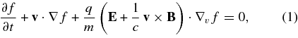
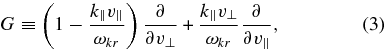
where E and B are the electric and magnetic fields, and ∇v is a gradient with respect to the velocity v. For most cases of interest, an analytic solution of the coupled Vlasov and Maxwell equations is not possible. On the other hand, in the case of a uniform plasma perturbed by small-amplitude, weakly damped waves, Equation (1) can be solved approximately using a standard technique known as quasilinear theory (Yakimenko 1963; Kennel & Engelmann 1966; Stix 1992). When this theory is applied to a plasma pervaded by a uniform background magnetic field  , and when there is no background electric field, each particle's orbit is approximated as the unperturbed helix that would arise in the absence of wave excitation. A first-order perturbation to f is then calculated, and the right-hand side of Equation (1) is averaged over a large volume V, yielding the following equation for the (averaged) distribution function (Kennel & Engelmann 1966),
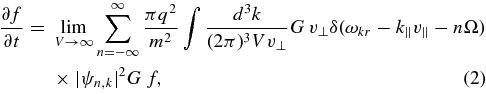
where v∥ (v⊥) is the component of v parallel (perpendicular) to B0,
ωkr is the real part of the wave frequency at wave vector k, Ω = qB0/mc is the cyclotron frequency, k∥ (k⊥) is the component of k parallel (perpendicular) to B0,
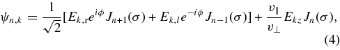
Jn is the Bessel function of nth order, σ = k⊥v⊥/Ω, ϕ is the azimuthal angle in wavenumber space,  ,
,  , and Ek is the Fourier transform of the electric field, given by ∫E(x, t)exp(−ik · x) d3x.1
Although Equation (2) is itself difficult to solve in many cases, two important results can be obtained even when the full solution for f is not available. These results are illustrated in Figure 1. First, for particles with parallel velocity v∥, the delta function in Equation (2) restricts the integral to waves satisfying the resonance condition

where n is any integer. The left-hand side of Equation (5) is the Doppler-shifted wave frequency seen in the frame of reference moving along B0 at velocity v∥. If this Doppler-shifted frequency is an integer multiple of Ω, then the effects of the wave's electromagnetic field on the particle add coherently over successive wave periods, and the wave has a large effect on the particle.

Figure 1. Shaded rectangles enclose portions of velocity space in which particles resonate with a wave with frequency ω and parallel wavenumber k∥. In quasilinear theory, particles interacting with such a wave diffuse in velocity space along semi-circular paths centered on the velocity coordinates v∥ = ωkr/k∥ and v⊥ = 0.
Download figure:
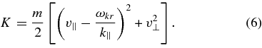
Standard image High-resolution imageSecond, at each point in velocity space the operator G is proportional to a derivative in a particular direction in the v∥ − v⊥ plane. This direction is along a semi-circular curve of constant particle energy K as measured in a frame of reference moving at the wave phase velocity along the background magnetic field  , where
Because the operator G appears twice, Equation (2) implies that each wave causes resonant particles to diffuse in velocity space along a curve of constant K. If particles throughout a broad range of v∥ interact with a spectrum of waves at different k∥ and ωkr, but all the waves have the same value of ωkr/k∥, then the particles can diffuse a substantial distance in velocity space while conserving K. The reason that K is conserved in this case is the following. In the reference frame moving at velocity  , the magnetic field is independent of time, and Faraday's law thus implies that ∇ × E = 0, so that E = −∇Φ, where Φ is the electrostatic potential. As a consequence, the change in a particle's kinetic energy is equal and opposite to the change in the particle's electrostatic potential energy. Since there is no background electric field in this reference frame, the variations in Φ are bounded and small. The particle's kinetic energy in this reference frame thus undergoes only small-amplitude oscillations and does not increase or decrease secularly in time.
3. PROTON INTERACTIONS WITH "SLAB" A/IC WAVES
We consider Alfvén/ion-cyclotron (A/IC) waves in a low-β, proton–electron plasma of density ρ0 pervaded by a uniform magnetic field  . We assume that the real part of the wave frequency, ωkr, is given by the cold-plasma dispersion relation (Stix 1992, Chapter 2, Equation (21); Hollweg 2000),
where
Ωp is the proton cyclotron frequency,
 is the Alfvén speed, and θ is the angle between k and B0. In Equation (7), we have neglected terms proportional to v2A/c2, me/mp, and (me/mp)tan2θ, where me and mp are the electron and proton masses.
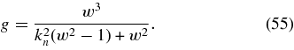
The root of Equation (7) corresponding to A/IC waves with θ = 0 (i.e., "slab waves") is given by
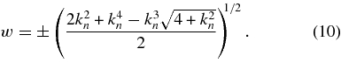
For kn ≫ 1, the right-hand side of Equation (10) can be expanded in powers of k−2n to yield

Through order k−4n, Equation (11) is equivalent to the approximate solution w ≃ 1 − (k2n + 2)−1 obtained by Hollweg (1999e).
When only waves with θ = 0 are present, the only nonvanishing terms in the sum on the right-hand side of Equation (2) are the n = 1 and n = −1 terms. This is because Jn(0) = 0 unless n = 0, and also because we have set me/mp → 0, which implies that Ekz = 0. In Figure 2, we plot the A/IC wave frequency in Equation (10) (solid lines) as well as the approximate expression for ωkr given in Equation (11) (dashed lines). The dotted lines are plots of nΩp + k∥v∥ for n = ±1 and v∥ = ∓0.03vA. For simplicity, we focus on positive k∥; the discussion and plots are unchanged if one sets k∥ → −k∥, ωkr → −ωkr, and n → −n. For each (nonzero) value of v∥ there is a unique value of |k∥|, denoted k∥,res, that satisfies the resonance condition for protons (i.e., Equation (5) with Ω = Ωp). This "resonant wavenumber" corresponds to the intersection of the dotted and solid lines.2 As illustrated in the figure, protons with positive v∥ resonate with A/IC waves with negative parallel phase velocity ωkr/k∥, while protons with v∥ < 0 resonate with A/IC waves with ωkr/k∥>0 (Dusenbery & Hollweg 1981).
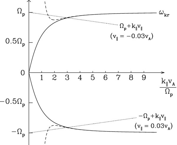
Figure 2. Solid lines plot the dispersion relation for slab A/IC waves from Equation (10). The dashed lines plot the approximate expression for ωkr in Equation (11). The intersections between the dotted lines and solid lines correspond to the solutions of Equation (5) for n = ±1 and Ω = Ωp.
Download figure:
Standard image High-resolution imageIt can also be seen from Figure 2 that protons with very large |v∥| resonate with waves with small |k∥|, for which |ωkr/k∥| ∼ vA. On the other hand, as |v∥| decreases, k∥,res increases and |ωkr/k∥,res| decreases. The condition |v∥| ≪ vA implies that
In this limit, Equations (5) and (11) can be used to express kn∥,res as an asymptotic series in powers of |v∥|/vA,
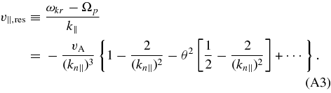
(The first term in this series was used as an approximation by Hollweg (1999e).) Equations (5), (11), and (13) can then be used to express the parallel phase velocity vph = ωkr/k∥ of the resonant waves as an asymptotic series in v∥/vA:
where the sign of vph(v∥) is the opposite of the sign of v∥.
As discussed in Section 2 and illustrated in Figure 1, a small-amplitude, weakly damped wave causes particles satisfying the resonance condition in Equation (5) to diffuse in velocity space along semi-circular paths of constant energy K as measured in the reference frame moving at velocity  . When many different waves are present, particles with a given velocity typically resonate with more than one wave at the same time, and the constant-K curves for the different resonant waves do not coincide. On the other hand, when only slab waves are present, each proton resonates with waves with only a single value of |k∥|. In this case, proton diffusion in the v∥ − v⊥ plane is one dimensional, in the sense that at each point in the v∥ − v⊥ plane protons diffuse along a single characteristic curve, and not in the direction perpendicular to this curve. We call these characteristic curves "scattering contours." Quantitatively, the equation describing these scattering contours can be written

where η is any function that satisfies the equation G(η) = 0 for waves with ωkr/k∥ = vph(v∥); i.e.,
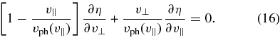
Equation (16) is solved by setting
where h satisfies the differential equation (Rowlands et al. 1966; Gendrin 1968)
For |v∥| ≪ vA, we can use Equations (14) and (18) to solve for h as an asymptotic series in powers of |v∥|/vA, from which we obtain
(A parametric solution for the η = constant surfaces was obtained by Isenberg & Lee (1996).) The shape of the η = 0.075v2A contour is plotted (solid line) in Figure 3. In this plot, v0=-0.08vA and v1 = −0.02vA, and vph(v0) and vph(v1) are obtained from Equation (14). At v∥ = v0, the constant-η contour is perpendicular to the dotted-line connecting the contour to the point [0, vph(v0)], reflecting the point made in Section 2, that the pitch-angle scattering at v0 occurs at constant energy as measured in the reference frame moving at velocity vph(v0) along B0. Similarly, at v∥ = v1, the constant-η contour is perpendicular to the dotted line connecting the contour to the point [0, vph(v1)].
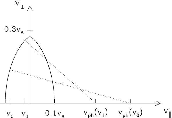
Figure 3. Solid-line curve shows the η = 0.075v2A scattering contour, where η is given by Equation (19). The dotted lines are perpendicular to the scattering contour, since particles with parallel velocity v∥ diffuse in velocity space along paths of constant energy in the reference frame moving at velocity vph(v∥) along the magnetic field.
Download figure:
Standard image High-resolution imageIf protons interact with a broad spectrum of A/IC waves, all with θ = 0, and if the proton distribution function f is initially Maxwellian, then the protons will diffuse in velocity space along the η = constant scattering contours, resulting in a net increase in average value of v2⊥. The energy gained by protons is removed from the waves, causing the waves to damp. However, in the limit of strong wave pitch-angle scattering, f will eventually become constant along the scattering contours, the protons will stop gaining energy from the waves, and the wave damping will cease (Kennel & Petschek 1966).
4. SECONDARY AMPLIFICATION OF SLAB WAVES AFTER f IS MODIFIED BY OBLIQUE WAVES
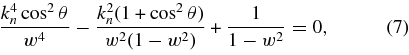
In this section, we argue that if the evolution of the proton distribution is dominated by resonant interactions with A/IC waves, and if the A/IC wave vectors are distributed over a range of directions, then the proton distribution function will (at least initially) become so anisotropic that A/IC waves with θ = 0 become unstable and grow. As in the previous section, we assume that ωkr is given by the cold-plasma dispersion relation and take the proton distribution to be confined to highly sub-Alfvénic parallel velocities, so that resonant wave–particle interactions arise only for k2n∥ ≫ 1 and |w| ≃ 1, where
In this limit, the solution to Equation (7) can be expressed as an asymptotic series in powers of |kn∥|−2,
In general, for A/IC waves with nonzero θ, one has to take into account wave–particle resonances with |n| ≠ 1 in Equation (5). However, for A/IC waves and protons with |v∥| ≪ vA, these resonances occur only for extremely large wavenumbers, |kn∥| ∼ vA/|v∥|, while the n = ±1 resonances arise for smaller wavenumbers, |kn∥| ∼ (vA/|v∥|)1/3. We assume that the power spectrum of A/IC waves decreases rapidly with increasing |kn∥| at |kn∥| ≳ (vA/|v∥|)1/3 due to wave damping. We thus neglect resonances with |n| ≠ 1. Using Equations (5) and (21) with n = ±1, we find that the value of |kn∥| for which A/IC waves with a given θ resonate with protons with a given v∥ is, to leading order in |v∥|/vA,
The parallel phase velocity ωkr/k∥ of the waves that are resonant with particles of parallel velocity v∥ is then, to leading order in |v∥|/vA,
The resonance condition requires that the sign of vph be the opposite of the sign of v∥, as for waves with θ = 0. In this section we use a different notation than in Equation (14), in that we now take vph to be a function of both v∥ and θ.
The key point to emerge from Equation (23) is that |vph| is an increasing function of θ at fixed v∥ for 0 < θ < 90°. One of the consequences of this point is illustrated in the top panel of Figure 4. In this panel, we take the proton distribution to be constant along the scattering contours corresponding to the slab waves. The scattering contour for η = 0.075v2A is shown as a solid-line curve. Protons at v∥ = v0 that are scattered by oblique A/IC waves with some nonzero value of θ will scatter along the dashed-line trajectory, which corresponds to constant energy as measured in a reference frame moving at velocity vph(v0, θ) along the magnetic field. (We note that we have artificially increased vph(v0, θ) relative to vph(v0, 0) in both panels of Figure 4 to make the figure easier to read.) If we take f to be a decreasing function of η, then there will be a net diffusive flux of protons upward along this dashed line, resulting in an increase in particle energy and damping of oblique waves.

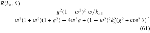
Figure 4. Upper panel: the proton distribution is taken to be constant along the η = constant scattering contours for waves with θ = 0, and to decrease as one moves to contours that are farther from the origin. The solid line is the η = 0.075v2A contour. Protons interacting with oblique waves will diffuse upward along the dashed line, gaining energy, and damping the oblique waves. Bottom panel: the proton distribution function is now taken to be constant along the scattering contours for oblique waves with some nonzero θ, and to decrease as one moves to contours that are farther from the origin. The solid line illustrates one such contour. Protons interacting with waves with θ = 0 will diffuse down the density gradient along the short-dashed line, losing energy, and amplifying the θ = 0 waves. The long-dashed line is a contour of constant energy in the plasma frame. Reprinted with permission from Pongkitiwanichakul, P., Chandran, B., Isenberg, P., & Vasquez, B. 2010, Resonant interactions between photons and Alfvén/Ion-cyclotron waves, 12th International Solar Wind Conference, AIP Conf. Proc., Volume 1216, pp 72–75. Copyright 2010, American Institute of Physics.
Download figure:
Standard image High-resolution imageA second consequence of Equation (23) is illustrated in the bottom panel of Figure 4. Here, we take the proton distribution to be constant along the scattering contours or "kinetic shells" corresponding to waves with a single nonzero value of θ. One of these contours is now drawn with a solid line. Protons at v∥ = v0 interacting with A/IC waves with θ = 0 will scatter along the short-dashed line in this panel, which locally corresponds to an η = constant curve, with η defined in Equation (19). If we take the proton distribution to decrease as one moves to shells that are farther from the origin, then there will be a net diffusive flux of protons downward along the short-dashed line in the bottom panel of Figure 4. In this case, the protons will lose energy, and waves with θ = 0 will be amplified.
If some mechanism such as plasma instabilities or a turbulent cascade generates high-frequency A/IC waves with a range of θ values, and if the form and evolution of the proton distribution function are dominated by wave–particle interactions, then interactions involving waves with nonzero θ will initially act to make the constant-f contours somewhat steeper in the v∥ − v⊥ plane than the η = constant scattering contours of the slab waves. This in turn will lead to the amplification of waves with θ = 0 and cause the angular distribution of the waves at large kn that resonate with the protons to become sharply peaked around θ = 0. Wave–particle interactions will subsequently become dominated by waves with θ = 0, f will become approximately constant along surfaces of constant η, and oblique waves will be damped. Numerical evidence supporting these arguments has recently been presented by Pongkitiwanichakul et al. (2010). We note that the damping of oblique waves coupled with the amplification of slab waves represents a kinetic mechanism for transporting wave energy toward θ = 0. In the next section, we analytically calculate γk assuming f = f(η).
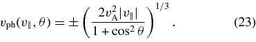
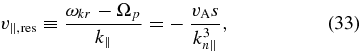
5. PROTON DAMPING OF OBLIQUE ALFVÉN/ION-CYCLOTRON WAVES WHEN f = f(η)
In this section, we consider a low-β proton–electron plasma in which f = f(η), where f is the proton distribution function and η is given by Equation (19). We then calculate the proton contribution to the damping rate of A/IC waves with θ ≠ 0. We denote the proton and electron contributions to the damping rate γ(p)k and γ(e)k, respectively. We assume that θ = 0 waves are present with both positive and negative values of ωkr/k∥, so that the scattering contours depicted in Figure 3 are filled for both positive and negative v∥. We assume that the total damping rate at wavevector k,
satisfies the inequality

for all n. If f were Maxwellian, this assumption would break down throughout a range of wavevectors in which |ωkr| is close to Ωp. (Stawicki et al. 2001; Gary & Borovsky 2004) However, because f = f(η), γ(p)k vanishes at all k at θ = 0, and is ≪|ωkr − nΩp| at all k and for all n if θ is sufficiently small. It is not clear a priori that Equation (25) is valid at all values of θ, but the results of our calculation are consistent with Equation (25), at least for θ ⩽ 45°.3
When Equation (25) is satisfied, the proton contribution to the damping rate is (see Kennel & Wong 1967)
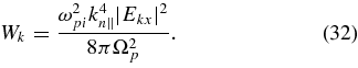
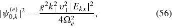
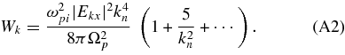
where N is the proton number density, ω2pi = 4πNe2/mp is the proton plasma frequency, mp and e are the proton mass and charge, G is defined in Equation (3),
Ek and Bk are the spatial Fourier transforms of the electric and magnetic fields,  h is the hermitian part of the dielectric tensor, which we approximate using the dielectric tensor for a cold plasma, and the frequency in Equation (27) is evaluated at ω = ωkr. The quantity ψ(p)n,k is equal to the quantity ψn,k defined in Equation (4) with Ω set equal to Ωp. Given the Fourier transform convention described following Equation (4) and in footnote 1, the wave energy (electromagnetic plus kinetic) per unit volume is limV→∞ (2π)−3 V−1∫2Wkd3k (see Equations (20) and (67) in Stix 1992, Chapter 4), and its rate of change is limV→∞ (2π)−3 V−1∫4γkWkd3k. Adding this to the rate of change of the proton energy per unit volume 0.5mp∫v2(∂f/∂t) d3v with ∂f/∂t given by Equation (2), and integrating by parts, one finds that the sum of the wave energy and proton energy limV→∞ (2π)−3 V−1∫2Wkd3k + 0.5mp∫v2f d3v remains constant. As in Section 3, we neglect terms of order me/mp when determining the dispersion relation and polarization properties of the waves. There is thus no parallel electric field fluctuation.
In general, for oblique waves, one has to include all the terms in the sum over n in Equation (26). However, we take the typical proton parallel velocity, v∥,th, to be ≪vA. As shown in Equation (22), the resonance condition for n = ±1 can be satisfied by the bulk of the protons for kn∥ ∼ (vA/v∥,th)1/3. In contrast, the resonance condition for |n| ≠ 1 can only be satisfied by the bulk of the protons for much larger wavenumbers, kn∥ ∼ vA/v∥,th, as discussed in the previous section. Moreover, we find that the damping rate decreases rapidly with increasing kn∥ for kn∥ ≳ (vA/v∥,th)1/3. Anticipating our discussion below, this is primarily because as kn∥ increases, ωkr → Ωp, and the wave energy becomes increasingly dominated by the kinetic energy of the oscillating proton fluid velocity, so that |Ekx|2/Wk decreases. The damping caused by resonant protons interacting with the wave electric field then becomes energetically less important, and the damping rate drops. We thus focus on proton damping at wavenumbers kn∥ ≪ vA/v∥,th, for which the n = ±1 resonances dominate, and neglect resonances with |n| ≠ 1. On the other hand, we take advantage of the fact that k2n∥,res ∼ (vA/|v∥|)2/3 ≫ 1 and calculate γ(p)k as an asymptotic series in powers of (1 − w), or equivalently k−2n∥, keeping only the leading-order term. Since we treat k2n∥ as large, and since we neglect the |n| ≠ 1 resonances which arise at kn∥ ≳ vA/v∥,th, our analysis is restricted to the wavenumber range
Without loss of generality, we consider waves with ωkr>0 and k∥>0, which resonate with protons with v∥ < 0. (The value of |γ(p)k/ωkr| is unchanged if we take ωkr/k∥ < 0 since the proton distribution is symmetric in v∥.) The damping rate is independent of ϕ, and so we set ϕ = 0, ky = 0, and kx = k⊥. To leading order in (1 − w), the polarization of A/IC waves is given by (Stix 1992, Chapter 2, Equation (28))

The recurrence relations 2nJn(x)/x = Jn−1(x) + Jn+1(x) and 2J'n(x) = Jn−1(x) − Jn+1(x), together with Equation (29), imply that
where
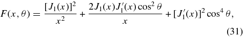
and J'n(x) = dJn(x)/dx. Using Equation (21) above and Equation (18) from Chapter 1 of Stix (1992), and neglecting terms proportional to me/mp, we find that to leading order in k−2n∥,
(The derivation of Equation (32) is described in Section 6.) Equation (21) implies that to leading order in k−2n∥,
where
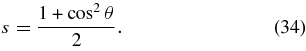
After setting f = f(η), we obtain
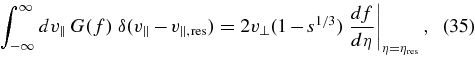
where

Since we have taken ωkr>0, we can neglect the n=−1 term in Equation (26), and keep only the n = 1 term. Substituting Equations (30) through (35) into Equation (26), we obtain
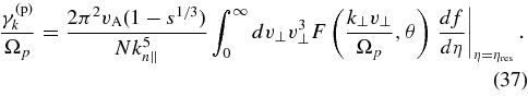
As an example, we set

with η0 ≪ v2A. The condition N = ∫d3vf then implies that to leading order in η0/v2A,
where Γ is the Gamma function. For this proton distribution function, Equation (37) and the Bessel-function identities on pp. 257–258 of Stix (1992) imply that
where
is roughly the square of k⊥ρp for the bulk of the protons, ρp is the proton gyroradius,
I1(λ) = (λ/2)(1 + λ2/8 + ⋅ ⋅ ⋅) is the modified Bessel function of order 1, and I'1(λ) = dI1(λ)/dλ.
To simplify our results further, we consider the limit
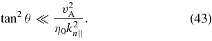
For the values of kn∥ at which γ(p)k is maximal, i.e., kn∥ ∼ v1/2A/η1/40, the inequality in Equation (43) is satisfied at most values of θ but is not satisfied when θ is very close to 90°. Equation (43) implies that

In this limit, to leading order in λ, H(λ, θ) = 2s2, and
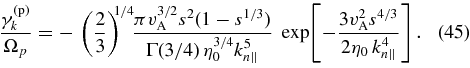
For fixed |θ|, the maximum value of |γ(p)k|, denoted γ(p)max, occurs at kn∥ = kn∥,max, where
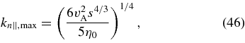
and is given by
We define the perpendicular and parallel thermal velocities v⊥,th and v∥,th such that f(v⊥,th, 0) = f(0, v∥,th) = (1/e)f(0, 0). Equations (19) and (38) then imply that v⊥,th = η1/20 and v∥,th = (2η0/3v2/3A)3/4, where in this last expression we have neglected the last term in Equation (19) since it is small. As a numerical example, we take v⊥,th = 200 km s-1 and vA = 2000 km s-1 and plot |γ(p)k|/ωkr at θ = 45°, 30°, and 10° in Figure 5, and γ(p)max/Ωp in Figure 6. For these parameters, v∥,th = 47 km s-1. For comparison, we also plot the electron damping rate, which is discussed in Section 6. As can be seen in Figure 5, the argument of the exponentials in Equations (40) and (45) causes the damping rate to drop rapidly as kn∥ is decreased below ∼v1/2A/η1/40 ≃ 3, because in this case there are exponentially few protons moving fast enough along the magnetic field to satisfy the resonance condition. On the other hand, γ(p)k is a rapidly decreasing function of kn∥ at kn∥ ≳ v1/2A/η1/40, primarily because γ(p)k is proportional to the energy in the electric field of the resonant waves divided by the wave energy, and |Ekx|2/Wk ∝ k−4n∥ at large kn∥ since the wave energy becomes dominated by proton kinetic energy as ωkr → Ωp.
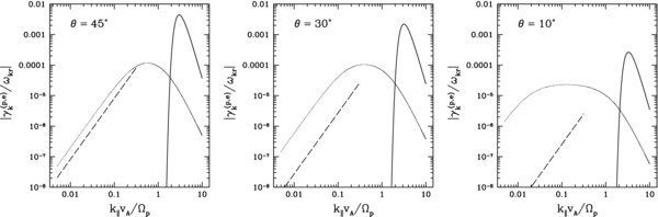
Figure 5. Proton (solid line) and electron (dotted line) contributions to the damping rate, γ(p)k and γ(e)k, from Equations (45) and (59) evaluated at θ = 45°, 30°, and 10°, assuming  , η0 = 0.01v2A, and βe = 0.01. The dashed-line is the electron damping rate from Equation (5) of Gary & Borovsky (2004) (quoted in Equation (62) below) for these same values of θ and βe.
Download figure:
Standard image High-resolution image
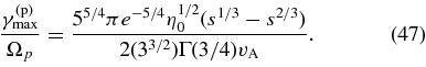
Figure 6. Maximum of |γ(p)k| from Equation (47) assuming  with η0 = 0.01v2A.
Download figure:
Standard image High-resolution imageIn the Appendix, we calculate the next higher-order term in powers of k−2n in the asymptotic expansion of γ(p)k in the limit that θ ≪ 1. This higher-order correction can be viewed as an estimate of the error in our leading-order result.
6. ELECTRON DAMPING OF OBLIQUE A/IC WAVES
In this section, we calculate the electron contribution to the damping rate of oblique A/IC waves, γ(e)k. We consider wavenumbers satisfying the inequality k∥vte ≪ Ωe, where Ωe and vte are the electron gyrofrequency and thermal speed. Since, k∥vte ≪ Ωe and ωkr ≪ Ωe, electrons interact with A/IC waves only through the n = 0 "Landau resonance" in Equation (5). In general, this resonance leads to two types of wave–particle interactions: Landau damping and "transit-time damping." In Landau damping, particles are pushed along the magnetic field by the wave electric field Ekz, whereas in transit-time damping particles are pushed along field lines by the μ∇B force of the waves. In our analysis, we neglect terms of order me/mp when determining the polarization properties of the waves. As a result, Ekz = 0 in our calculation, and there is no Landau damping. Gary & Borovsky (2004) showed that the contributions to γ(e)k from electron transit-time damping and Landau damping have the same order of magnitude for θ ≲ 45°, but that electron Landau damping becomes much stronger than electron transit-time damping as θ is increased from ∼45° toward 90°. The expression we derive for γ(e)k is thus only a reasonable approximation of the actual electron damping rate for θ ≲ 45°, as discussed further below.
We assume that |γk/ωkr| ≪ 1, so that the electron contribution to the damping rate is (Kennel & Wong 1967)
where N and Wk are defined in the previous section, ω2pe = 4πNe2/me is the square of the electron plasma frequency, sgn(x) ≡ x/|x|, v⊥ and v∥ are the velocity components perpendicular and parallel to B0,
is the Maxwellian electron distribution function, and Te is the electron temperature. The quantity ψ(e)n,k is equal to the quantity ψn,k defined in Equation (4) with Ω set equal to Ωe.
To determine the dispersion relation and wave polarization properties, we use the cold-plasma approximation. The cold-plasma dispersion relation in the A/IC frequency range is given by Equation (7), which neglects terms of order v2A/c2, me/mp, and (me/mp)tan2θ. The A/IC frequency is obtained by solving Equation (7) for w2 and choosing the minus sign in the quadratic formula, which gives
The damping rate is independent of the azimuthal angle ϕ in k-space, and so we take ϕ = 0 and  . The transverse components of the electric-field fluctuation are then related by the equation (Stix 1992)
where S and iD are the xx and yx components of the dielectric tensor. The general definitions of S and D are given in Equations (19) through (21) from Chapter 1 of Stix (1992). Neglecting terms of order me/mp, v2A/c2, and (me/mp)tan2θ, we find that for A/IC waves,
and
Equations (51) through (53) can be rearranged to yield

where
Equations (4) and (55) imply that
where we have made use of the inequality k⊥v⊥/Ωe ≪ 1 and employed the approximation that J1(x) ≃ x/2 when x ≪ 1. To calculate Wk in Equation (27), we use the cold-plasma approximation for the dielectric tensor,
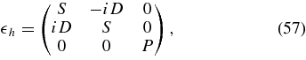
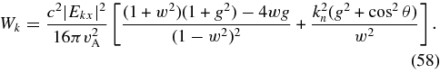
where S and D are given in Equations (52) and (53), and P ≃ −ω2pe/ω2kr. Faraday's law implies that B*k · Bk = c2k2n|Ekx|2(g2 + cos2θ)/(v2Aw2). Equations (27), (54), and (57) then imply that
Equation (32) follows from Equation (58) in the limit that k2n∥ ≫ 1. After substituting Equations (56) and (58) into Equation (48), we find that
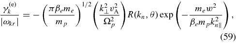
where

and
The exponential in Equation (59) implies that when βe ≪ me/mp, the damping rate becomes exponentially small at kn∥ ≲ 1 where w/kn∥ ∼ 1 because there are extremely few electrons with v∥ ≃ ±vA.
Equation (59) can be compared with Equation (5) of Gary & Borovsky (2004),
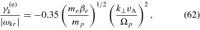
which was obtained by fitting numerical results for the damping rate at k∥ ≃ kd/3, where kd ≃ Ωp/vA is the wavenumber corresponding to the rapid onset of proton cyclotron damping. Gary & Borovsky (2004) argued that Equation (62) is approximately valid for most wavenumbers satisfying k∥ < kd, which is consistent with Figure 4 of Cranmer & van Ballegooijen (2003), which suggests that γ(e)k is independent of k∥ for |k∥| ≪ kd. Our results, however, suggest that γ(e)k departs from the scaling in Equation (62) as k∥ is increased from kd/3 to kd (at least when the proton distribution function satisfies f = f(η) so that |γ(p)k| ≪ |ωkr|), and thus we take Equation (62) to apply only for k∥ < kd/3 ≃ Ωp/(3vA).4 In the limit |kn∥| ≪ sin2θ, R(kn, θ) ≃ (cos4θ)/(2sin4θ), and Equation (59) becomes
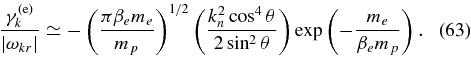
We emphasize that Equation (63) is not the proper limit of Equation (59) as θ → 0, since Equation (63) assumes that sin2θ ≫ |kn∥|. If βe>me/mp, then the exponential in Equation (63) is ∼1, and Equation (63) is similar to Equation (62) for θ ≃ 45°. However, the damping rates in these two equations scale differently with θ. For θ significantly larger than 45°, our result for γ(e)k is smaller than that of Gary & Borovsky (2004), and we do not view our result as reliable for this range of θ because of our neglect of Landau damping and finite-Larmor-radius effects on the wave properties. For θ < 45°, we find that the electron damping rate is larger than in the analysis of Gary & Borovsky (2004). Although their result is based on numerical solutions to the full hot-plasma dispersion relation, it is not clear that their result is to be preferred at small θ, because almost all of the numerical data used to obtain Equation (62) corresponded to wave vectors satisfying θ>45°. We thus take Equation (59) to be reasonably accurate for θ < 45°.
Equation (59) implies that as kn∥ increases above ∼1, the electron contribution to the damping rate decreases. As in the case of the proton cyclotron damping rate, this is primarily because |Ekx|2/Wk decreases with increasing |kn∥|, since the the wave energy becomes dominated by proton kinetic energy as ωkr → Ωp. The values of γ(e)k/|ωkr| in Equation (59) at θ = 45°, 30°, and 10° are plotted in Figure 5 for βe = 0.01. For comparison, the result of Gary & Borovsky (2004) in Equation (62) is plotted in these figures as well. It can be seen that at these values of θ the maximum value of |γ(p)k/ωkr| is a factor of ∼10 − 40 larger than the maximum value of |γ(e)k/ωkr| from Equation (59). We note that we are comparing the damping rate for an "evolved" proton distribution to the damping rate for an "un-evolved" electron distribution. It is possible that the electron distribution will evolve in such a way that the electron damping rate of A/IC waves is reduced relative to the case of Maxwellian electrons, in particular, by flattening (i.e., reducing |∂fe/∂v∥|) at |v∥| < vA.
7. PROTON HEATING VIA THE DISSIPATION OF HIGH-FREQUENCY A/IC-WAVE TURBULENCE
If nonlinear wave–wave interactions cause A/IC-wave energy to cascade to larger k∥, then this energy cascade will be truncated by wave damping once it reaches a wavenumber at which γkτk ≳ 1, where τk is the energy cascade time, i.e., the timescale on which energy at wavenumber k is transferred to wavenumber 2k. In the solar corona and solar flares, δBk/B0 is very small for kn>1, where δBk is the rms amplitude of the magnetic field fluctuation at scale k−1. As a result, high-frequency A/IC waves at kn>1 and |ω| ∼ Ωp are weakly turbulent, with τk ≫ ω−1kr. (Zakharov et al. 1992) Thus, although γ(p)k in Equation (37) is ≪ωkr, γ(p)kτk may nevertheless exceed 1 near the maximum (in kn) of γ(p)k. If it does, then proton damping is sufficient to terminate the cascade. As shown in Figure 5, the maximum electron damping rate is much less than the maximum proton damping rate, at least for moderately oblique waves. If the proton damping rate is sufficient to truncate the cascade but the electron damping rate is not, then most of the turbulent power will go into proton heating, at least for A/IC waves with θ ≲ 45°. On the other hand, if the turbulence amplitude is so small that γ(e)kτk>1 at kn∥ ≲ 1, then the cascade would be truncated by electron damping at kn∥ < 1 before it reaches sufficiently high kn∥ that proton cyclotron damping becomes important.
A thorough description of the above scenario is, however, beyond the scope of this paper. One complication is that the dissipation scenario just described involves the amplification of A/IC waves with θ = 0, and the processes that drain A/IC-wave energy at θ = 0 from the system (e.g., propagation out of the system, cascade, phase mixing (Heyvaerts & Priest 1983), or damping) need to be identified and modeled. Another source of uncertainty concerns the value of τk at the scales of interest in collisionless plasmas such as the solar corona and solar flares. Recent studies have begun to address the cascade of Alfvén-wave energy to large k∥ at frequencies ≪Ωp (Chandran 2005, 2008; Luo & Melrose 2006) as well as the way in which slow magnetosonic waves can cause A/IC waves with θ = 0 to cascade to larger k∥ (Yoon & Fang 2008). However, the cascade of A/IC-wave energy to larger k∥ at k∥ ≳ Ωp/vA in collisionless plasmas, in which slow waves are strongly damped, is still not well understood.
8. CONCLUSION
In this paper, we consider resonant interactions between protons and oblique A/IC waves for the case in which the proton distribution function f is strongly modified by wave pitch-angle scattering. We argue that wave–particle interactions involving oblique waves cause f to become unstable to waves with θ = 0, where θ is the angle between the wave vector and the background magnetic field. The resulting amplification of A/IC waves with θ = 0 causes the angular distribution of A/IC waves to become sharply peaked about θ = 0 at the large wavenumbers at which protons resonate with A/IC waves. Wave–particle interactions then cause f to become approximately constant along the set of closed, nested scattering contours corresponding to waves with θ = 0, which are defined by the equation η(v⊥, v∥) = constant, with the approximate value of η given in Equation (19). Once f = f(η), oblique A/IC waves continue to be damped by protons. The damping of oblique waves coupled with the amplification of θ = 0 waves represents a kinetic mechanism for the spectral transport of wave energy toward θ = 0. Because the plasma does not relax to a state in which proton damping of oblique A/IC waves ceases, oblique high-frequency A/IC waves can be significantly more effective at heating protons than A/IC waves with θ = 0. In sections 5 and 6 we analytically calculate the approximate values of the proton and electron contributions to the damping rate of oblique A/IC waves, assuming Maxwellian electrons and f = f(η). As shown in Figure 5, the peak proton damping rate is much larger than the peak electron damping rate for moderately oblique waves. As a result, in at least some circumstances most of the heating power that results from the dissipation of moderately oblique, high-frequency A/IC waves will be deposited into the protons.
This work was supported in part by DOE Grant DE-FG02-07-ER46372, NSF Grant AGS-0851005, NSF-DOE Grants AST-0613622 and AGS-1003451, and NASA Grants NNX07AP65G, NNX08AH52G, NNX09AJ80G, and NNX07AI14G.
APPENDIX: HIGHER-ORDER TERMS IN THE ASYMPTOTIC SERIES FOR γ(P)k AT θ ≪ 1
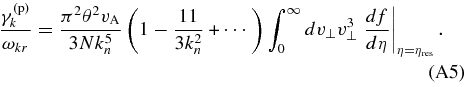
In this Appendix, we calculate γ(p)k as an asymptotic series in both θ and k−2n, keeping only the leading-order term in θ, the leading-order term in k−2n, and the first-order correction in k−2n. By calculating the first-order correction in k−2n, and viewing this correction as an estimate of the error in the leading-order result, we can gain some insight into how accurate Equations (40) and (45) are for parameters of interest, at least for small θ.
The solution to Equation (7) can be expressed as the asymptotic series,
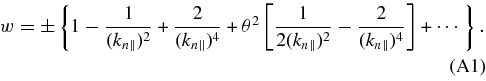
At θ = 0, Eky = −iEkx exactly at all kn for A/IC waves (Stix 1992). To leading order in θ, |ψ(p)1,k|2 = |Ekx|2 to all orders in k−1n, and
Equation (A1) implies that
After setting f = f(η), we obtain

where ηres = η[v⊥, v∥,res(kn∥, 0)]. Noting that to lowest order in θ, kn and kn∥ are interchangeable, we finally obtain
As an example, we again set

with η0 ≪ v2A. The condition N = ∫d3vf then implies that
where Γ is the Gamma function, and the dots (⋅⋅⋅) represent higher-order corrections in powers of η1/20/vA, which we neglect. Using Equations (A6) and (A7) in Equation (A5), we obtain
where
Since the peak damping rates occur for ![$k_n \sim \sqrt{v_{\rm A}}/\sqrt[4]{\eta _0}$](https://content.cld.iop.org/journals/0004-637X/722/1/710/revision1/apj306174ieqn12.gif) , we treat kn and
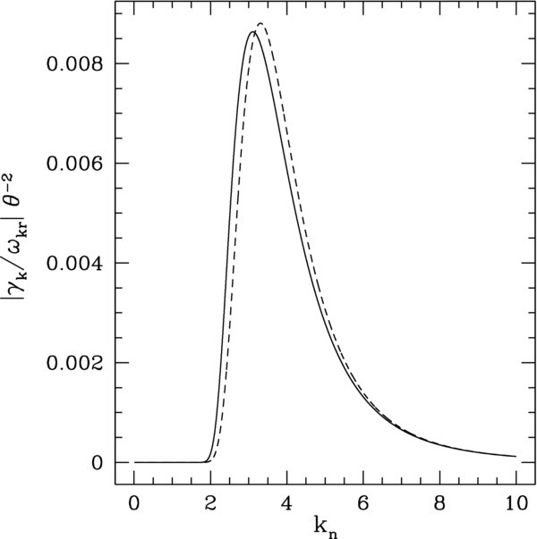
, we treat kn and ![$\sqrt{v_{\rm A}}/\sqrt[4] {\eta _0}$](https://content.cld.iop.org/journals/0004-637X/722/1/710/revision1/apj306174ieqn13.gif) as being of equivalent order. As in the previous section, we take v⊥,th = 200 km s-1 and vA = 2000 km s-1 and then plot the value of γ(p)k for these parameters in Figure 7. As seen in the figure, our results for γ(p)k at small θ are not changed very much when we go from keeping just the first term in powers of k−2n in the asymptotic series for γ(p)k to keeping both the first and second terms in this series.
as being of equivalent order. As in the previous section, we take v⊥,th = 200 km s-1 and vA = 2000 km s-1 and then plot the value of γ(p)k for these parameters in Figure 7. As seen in the figure, our results for γ(p)k at small θ are not changed very much when we go from keeping just the first term in powers of k−2n in the asymptotic series for γ(p)k to keeping both the first and second terms in this series.
Figure 7. Normalized damping rate |γ(p)k/ωkr| at θ ≪ 1 divided by θ2 for 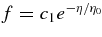 with η0 = 0.01v2A. The solid line is a plot of Equation (A8), and the dashed line gives just the leading-order result (i.e., Equation (A8) with δ = 0).
Download figure:
Standard image High-resolution image
Footnotes
- 1
Like Kennel & Engelmann (1966), we treat the plasma as infinite. Therefore, before taking a Fourier transform of a function of x, we first multiply the function by a "window function" that is 1 inside a cube of volume V and 0 outside this cube, where V is the same quantity that appears in Equation (2). This procedure is described in more detail by Stix (1992).
- 2
A/IC waves with θ = 0 satisfy Eky = −iEkxω/|ω|. It thus follows from Equations (33), (40), and (41) of chapter 17 of Stix (1992) that A/IC waves with θ = 0 and ω>0 resonate with ions only through the n = +1 resonance in Equation (5), while A/IC waves with θ = 0 and ω < 0 resonate with protons only through the n = −1 resonance in Equation (5), where we are taking Ekz = 0. Thus, although the dotted line in Figure 2 labeled Ωp + k∥v∥ would intersect the solid-line plot of ωkr at ωkr < 0 if extended to very large k∥, this second intersection does not correspond to an actual resonance with θ = 0 A/IC waves.
- 3
- 4
The discrepancy between Equation (59) and Equation (62) at k∥>kd/3 may be related to our assumption that the total damping rate γk satisfies |γk| ≪ |ωkr|. This assumption is reasonable when the proton distribution function satisfies f = f(η) as in Section 5, since then |γ(p)k| ≪ |ωkr|. However, when the protons are Maxwellian, as assumed by Gary & Borovsky (2004), |γ(p)k| ∼ |ωkr| at k∥ ≳ kd where ωkr ∼ Ωp. In this strong-damping limit, the wave dispersion and polarization properties are strongly modified relative to the cold-plasma limit, and the electron damping rate is not well described by Equation (59).