


ABSTRACT
Bulk dark energy (DE) properties are determined by the redshift evolution of its pressure-to-density ratio, wde(z). An experimental goal is to decide if the DE is dynamical, as in the quintessence (and phantom) models treated here. We show that a three-parameter approximation wde(z; εs, εϕ∞, ζs) fits well the ensemble of trajectories for a wide class of late-inflaton potentials V(ϕ). Markov Chain Monte Carlo probability calculations are used to confront our wde(z) trajectories with current observational information on Type Ia supernova, cosmic microwave background, galaxy power spectra, weak lensing, and the Lyα forest. We find that the best-constrained parameter is a low-redshift slope parameter, εs ∝ (∂ln V/∂ϕ)2 when the DE and matter have equal energy densities. A tracking parameter εϕ∞ defining the high-redshift attractor of 1 + wde is marginally constrained. ζs is poorly determined, which characterizes the evolution of εs, and is a measure of ∂2ln V/∂ϕ2. The constraints we find already rule out some popular quintessence and phantom models, or restrict their potential parameters. We also forecast how the next generation of cosmological observations improve the constraints: by a factor of about five on εs and εϕ∞, but with ζs remaining unconstrained (unless the true model significantly deviates from ΛCDM). Thus, potential reconstruction beyond an overall height and a gradient is not feasible for the large space of late-inflaton models considered here.
1. INTRODUCTION
1.1. Running Dark Energy and Its Equation of State
One of the greatest mysteries in physics is the nature of dark energy (DE) which drives the present-day cosmic acceleration, inferred to exist from supernovae (SNe) data (Riess et al. 1998; Perlmutter et al. 1999), and from a combination of cosmic microwave background (CMB) and large-scale structure (LSS) data (Bond & Jaffe 1999). Although there have been voluminous outpourings on possible theoretical explanations of DE, recently reviewed in Copeland et al. (2006), Kamionkowski (2007), Linder (2008a, 2008b), and Silvestri & Trodden (2009), we are far from consensus. An observational target is to determine if there are temporal (and spatial) variations beyond the simple constant Λ. Limits from the evolving data continue to roughly center on the cosmological constant case Λ, which could be significantly strengthened in near-future experiments—or ruled out. We explore the class of effective scalar field models for DE evolution in this paper, develop a three-parameter expression which accurately approximates the dynamical histories in most of those models, and determine current constraints and forecast future ones on these parameters.
The mean DE density is a fraction Ωde of the mean total energy density,

which is itself related to the Hubble parameter H through the energy constraint equation of gravity theory as indicated. Ωde(a) rises from a small fraction relative to the matter at high redshift to its current ∼0.7 value. Here , is the reduced Planck mass, GN is Newton's gravitational constant, and ℏ and c are set to unity, as they are throughout this paper.

Much observational effort is being unleashed to determine as much as we can about the change of the trajectory ρde with expansion factor a, expressed through a logarithmic running with respect to ln a:

This ρde-run is interpreted as defining a phenomenological average pressure-to-density ratio, the DE equation of state (EOS). The total "acceleration factor,"  ≡ 1 + q, where the conventional "deceleration parameter" is = −dln(Ha)/dln a, is similarly related to the running of the total energy density:


Equation (3) shows is the density-weighted sum of the acceleration factors for matter and DE. Matter here is everything but the DE. Its EOS has m = 3/2 in the non-relativistic-matter-dominated phase (dark matter and baryons) and m = 2 in the radiation-dominated phase.
1.2. The Semi-blind Trajectory Approach
We would like to use the data to constrain ρde(ln a) with as few prior assumptions on the nature of the trajectories as is feasible. However, such blind analyses are actually never truly blind, since ρde or wde is expanded in a truncated basis of mode functions of one sort or another: there will necessarily be assumptions made on the smoothness associated with the order of the mode expansion and on the measure, i.e., prior probability, of the unknown coefficients multiplying the modes. The most relevant current data for constraining wde, Type Ia Supernova (SNIa) compilations, extends back only about one e-folding in a, and probes a double integral of wde, smoothing over irregularities. The consequence is that unless wde was very wildly varying, only a few parameters are likely to be extractable no matter what expansion is made.
Low-order expansions include the oft-used but nonphysical cases of constant w0 ≠ −1 and the two-parameter linear expansion in a (Chevallier & Polarski 2001; Linder 2003; Wang & Tegmark 2004; Upadhye et al. 2005; Liddle et al. 2006; Francis et al. 2007; Wang et al. 2007),

adopted by the Dark Energy Task Force (DETF; see Albrecht et al. 2006). The current observational data we use in this paper to constrain our more physically motivated parameterized trajectories are applied in Figure 1 to w0 and wa, assuming uniform uncorrelated priors on each. The area of the nearly elliptical 1σ error contour has been used to compare how current and proposed DE probes do relative to each other; its inverse defines the DETF "figure of merit" (FOM; see Albrecht et al. 2009).

Figure 1. Marginalized 68.3% CL (inner contour) and 95.4% CL (outer contour) constraints on w0 and wa for the conventional DETF parameterization w = w0 + wa(1 − a), using the current data sets described in Section 4. The white point is the cosmological constant model. The solid red line is a slow-roll consistency relation, Equation (49) derived in Section 6.2 (for a fixed Ωm0 = 0.29, as inferred by all of the current data). The tilted dashed gray line shows wa = −1 − w0. Pure quintessence models restrict the parameter space to 1 + w0>0 and wa above the line, whereas in the pure phantom regime, 1 + w0 < −0 and wa would have to lie below the line. Allowing for equal a priori probabilities to populate the other regions is quite problematical theoretically, and indeed the most reasonable theory prior would allow only the pure quintessence domain.
Download figure:
Standard image High-resolution imageConstant wde and Equation (4) can be considered to be the zeroth- and first-order polynomial expansion in the variable 1 − a. Why not redshift z (Upadhye et al. 2005; Linder & Huterer 2005) or the scale factor to some power (Linder & Huterer 2005) or ln a? Why pivot about a = 1?
Why is it only linear in a? Why not expand to higher order? Why not use localized spline mode functions, the simplest of which is a set of contiguous top hats (unity in a redshift band, zero outside)? These cases too have been much explored in the literature, both for current and forecast data. The method of principal component (parameter eigenmode) analysis takes orthogonal linear combinations of the mode functions and of their coefficients, rank-ordered by the error matrix eigenmodes (see, e.g., Huterer & Starkman 2003; Crittenden & Pogosian 2005). As expected only a few linear combinations of mode function coefficients are reasonably determined. Thus, another few-parameter approach expands wde in many modes localized in redshift but uses only the lowest error linear combinations. At least at the linearized level, the few new parameters so introduced are uncorrelated. However, the eigenmodes are sensitive to the data chosen and the prior probabilities of the mode parameters. An alternative to the wde expansion is a direct mode expansion in , considered at low order by Rapetti et al. (2007); since the m part is known, this is an expansion in (de − m)Ωde, in which case wde becomes a derived trajectory; for wde parameterizations it is (a) that is the derived trajectory.
The partially blind expansions of 1 + wde are similar to the early universe inflation expansions of the scalar power spectrum (e.g., J. R. Bond et al. 2010, in preparation), except in that case one is "running" in "resolution," ln k. However, there is an approximate relation between the comoving wavenumber k and the time when that specific k-wave went out of causal contact by crossing the instantaneous comoving "horizon" parameterized by Ha. This allows one to translate the power spectra ln k-trajectories into dynamical ln Ha-trajectories, . The lowest order is a uniform slope ; next order is a running of that slope, rather like the DETF linear wde expansion. Beyond that, one can go to higher order, e.g., by expanding in Chebyshev polynomials in ln k, or by using localized modes to determine the power spectrum in k bands. Generally, there may be tensor and isocurvature power spectra contributing to the signals, and these would have their own expansions.


In inflation theory, the tensor and scalar spectra are related to each other by an approximate consistency condition: both are derivable from parameterized acceleration factor trajectories defining the inflaton EOS, 1 + wϕ(a) = 2/3 (with zero Ωm in early universe inflation). Thus, there is a very close analogy between phenomenological treatments of early and late universe inflation. However, there is a big difference: power spectra can be determined by over ∼10 e-foldings in k from CMB and LSS data on clustering, and hence over ∼10 e-foldings in a, whereas DE data probe little more than an e-folding of a. This means that higher order partially blind mode expansions are less likely to bear fruit in the late-inflaton case.
1.3. Physically Motivated Late-inflaton Trajectories
This arbitrariness in semi-blind expansions motivates our quest to find a theoretically motivated prior probability on general DE trajectories characterized by a few parameters, with the smoothness that is imposed following from physical models of their origin rather than from arbitrary restrictions on blind paths. Such a prior has not been much emphasized in DE physics, except on an individual-model basis. The theory space of models whose trajectories we might wish to range over include:
- 1.quintessence, with the acceleration driven by a scalar field minimally coupled to gravity with an effective potential with small effective mass and a canonical kinetic energy (Ratra & Peebles 1988; Wetterich 1988; Frieman et al. 1995; Binétruy 1999; Barreiro et al. 2000; Brax & Martin 1999; Copeland et al. 2000; de La Macorra & Stephan-Otto 2001; Linder 2006; Huterer & Peiris 2007; Linder 2008c);
- 2.
- 3.F(R, ϕ) models, with Lagrangians involving a function of the curvature scalar R or a generalized dilaton ϕ, that can be transformed through a conformal mapping into a theory with an effective scalar field, albeit with interesting fifth force couplings to the matter sector popping out in the transform (Capozziello & Fang 2002; Carroll et al. 2004; de La Cruz-Dombriz & Dobado 2006; Nojiri & Odintsov 2006; de Felice & Tsujikawa 2010; Sotiriou & Faraoni 2010); and
- 4.
In this paper, we concentrate on the quintessence class of models, but allow trajectories that would arise from a huge range of potentials, with our fitting formula only deviating significantly when |1 + wde|>0.5. A class of models that we do not try to include are ones with DE having damped oscillations before settling into a minimum Λ (Kaloper & Sorbo 2006; Dutta & Scherrer 2008).
We also extend our paths to include ones with wde < −1, the phantom regime where the null energy condition (Carroll et al. 2003) is violated. This can be done by making the kinetic energy negative, at least over some range, but such models are ill-defined. There have been models proposed utilizing extra UV physics, such as with a Lorentz-violating cutoff (Cline et al. 2004) or with extra fields (Sergienko & Rubakov 2008). Regions with wde < −1 are consistent with current observations, so a semi-blind phenomenology should embrace that possibility. It is straightforward to extend our quintessence fitting formula to the phantom region, so we do, but show results with and without imposing the theoretical prior that these are highly unlikely.
The evolution of wde for a quintessence field ϕ depends on its potential V(ϕ) and its initial conditions. For a flat Friedmann–Robertson–Walker (FRW) universe with given present matter density ρm0 and DE density ρde0, any function wde(a) satisfying 0 ⩽ 1 + wde ⩽ 2 can be reverse-engineered into a potential V(ϕ) and an initial field momentum, . (The initial field value ϕini can be eliminated by a translation in V(ϕ) and the sign of by a reflection in V(ϕ).) Given this one-to-one mapping between and {w(a), ρde0; ρm0}, we may think we should allow for all wde trajectories. Generally, these will lead to very baroque potentials indeed, and unrealistic initial momenta. The quintessence models with specific potentials that have been proposed in the literature are characterized by a few parameters, and have a long period in which trajectories relax to attractor ones, leading to smooth trajectories in the observable range at low redshift. These are the simple class of potentials we are interested in here: our philosophy is to consider "simple potentials" rather than simple mathematical forms of wde(a). The potentials which we quantitatively discuss in later sections include: power laws (Ratra & Peebles 1988; Steinhardt et al. 1999), exponentials (Ratra & Peebles 1988), double exponentials (Barreiro et al. 2000; Sen & Sethi 2002; Neupane 2004a, 2004b; Jarv et al. 2004), cosines from pseudo-Nambu Goldstone bosons (pnGB) (Frieman et al. 1995; Kaloper & Sorbo 2006), and supergravity (SUGRA) motivated models (Brax & Martin 1999). Our general method applies to a much broader class than these though: we find that the specific global form of the potential is not relevant because the relatively small motions on its surface in the observable range allow only minimal local shape characteristics to be determined, and these we can encode with the three key physical variables parameterizing our wde. Even with the forecasts data to come, we can refine our determinations but not gain significantly more information—unless the entire framework is shown to be at variance with the data.


1.4. Tracking and Thawing Models
Quintessence models are often classified into tracking and thawing models (Caldwell & Linder 2005; Linder 2006, 2008c; Huterer & Peiris 2007; Sullivan et al. 2007; Scherrer & Sen 2008). Tracking models were first proposed to solve the coincidence problem, i.e., why the DE starts to dominate not very long after the epoch of matter–radiation equality (∼7.5 e-folds). However, a simple negative power-law tracking model that solves the coincidence problem predicts wde ≳ −0.5 today, which is strongly disfavored by current observational data. In order to achieve the observationally favored wde ≈ −1 today, one has to assume the potential changes at an energy scale close to the energy density at matter–radiation equality. The coincidence problem is hence converted to a fine-tuning problem. In this paper, we take the tracking models as the high-redshift limit and parameterize it with a "tracking parameter" εϕ∞ that characterizes the attractor solution. The thawing models, where the scalar field is frozen at high redshift due to large Hubble friction, can be regarded as a special case of tracking models where the tracking parameter is zero. Because of the nature of tracking behavior, where all solutions regardless of initial conditions approach an attractor, we do not need an extra parameter to parameterize the initial field momentum.
In either tracking models or thawing models the scalar field has to be slowly rolling or moderately rolling at low redshift, so that the late-universe acceleration can be achieved. The main physical quantity that affects the dynamics of quintessence in the late-universe accelerating epoch is the slope of the potential. The field momentum is "damped" by Hubble friction, and the slope of the potential will determine how fast the field will be rolling down; actually, as we show here, it is the ϕ-gradient of ln V that matters, and this defines our second "slope parameter" εs.
It turns out that a two-parameter formula utilizing just εϕ∞ and εs works very well, because the field rolls slowly at low redshift, indeed is almost frozen, so the trajectory does not explore changes in the slope of ln V. However, we want to extend our formula to cover the space of moderate-roll as well as slow-roll paths. Moreover, in cases in which ln V changes significantly, even slow-roll paths may explore the curvature of ln V as well as its ϕ-gradient. Accordingly, we expanded our formula to encompass such cases, introducing a third parameter ζs, which is related to the second ϕ-derivative of ln V, explicitly so in thawing models.
1.5. Parameter Priors for Tracking and Thawing Models
Of course, there is one more important fourth parameter, characterizing the late-inflaton energy scale, such as the current DE density ρde,0 at redshift 0. This is related to the current Hubble parameter H0 ≡ 100 h kms−1Mpc−1, the present-day fractional matter density Ωm0, and the current fractional DE density ΩΛ ≡ Ωde,0 = 1 − Ωm0h2/h2: ρde,0 = 3Mp2H20ΩΛ. With CMB data, the sound-crossing angular scale at recombination is actually used, as is the physical density parameter of the matter, Ωm0h2, which is typically derived from separately determined dark matter and baryonic physical density parameters, Ωdm0h2 and Ωb0h2. With any nontrivial wde EOS, this depends upon the parameters of wde as well as on one of h or the inter-related zero redshift density parameters. The important point here is that the prior measure is uniform in the sound-crossing angular scale at recombination and in Ωdm0h2 and Ωb0h2, not in h or the energy scale of late inflation. If the quantities are well measured, as they are, the specific prior does not matter very much.
What to use for the prior probability of the parameters of wde, in which most are not well determined? The prior chosen does matter and has to be understood when assessing the meaning of the derived constraints. Usually a uniform prior in w0 and wa is used for the DETF form, Equation (4). The analog for our parameterization is to be uniform in the relatively well-determined εs, but we show what variations in the measure on it do, e.g., using or disallowing phantom trajectories, εs>0. The measure for each of the other two parameters is also taken to be uniform. (Our physics-based parameterization leads to an approximate "consistency relation" between w0 and wa, a strong prior relative to the usual uniform one.)

In Section 2, we manipulate the dynamic equations for quintessence and phantom fields to derive our approximate solution, wde(a|εs, εϕ∞, ζs, Ωm0). We show how well this formula works in reproducing full trajectories computed for a variety of potentials. In Section 4, we describe our extension of the CosmoMC program package (Lewis & Bridle 2002) to treat our parameterized DE and the following updated cosmological data sets: SNIa, galaxy power spectra that probe LSS, weak lensing (WL), CMB, and Lyα forest (Lyα). The present-day data are used to constrain our dynamical wde(a). In Section 5, we investigate how future observational cosmology surveys can sharpen the constraints on wde(a|εs, εϕ∞, ζs, Ωm0). We restrict our attention to flat universes. We discuss our results in Section 6.
2. LATE-INFLATION TRAJECTORIES AND THEIR PARAMETERIZATION
2.1. The Field Equations in Terms of Equations of State
We assume the DE is the energy density of a quintessence (or phantom) field, with a canonical kinetic energy and an effective potential energy V(ϕ). This is derived from a Lagrangian density

where "+" is for quintessence ("−" for phantom). Throughout this paper, we adopt the (+, −, −, −) metric signature. For homogeneous fields the energy density, pressure, and EOS are


Since we identify the DE with an inflaton, we hereafter use ϕ as the subscript rather than "de." The field ϕ does not have to be a fundamental scalar—it could be an effective field, an order parameter associated with some collective combination of fields. A simple way to include the phantom field case is to change the kinetic energy sign to minus, although thereby making it a ghost field with unpalatable properties even if it is the most straightforward way to get 1 + wde < 0.
The two scalar field equations, for the evolution of the field, , and of the field momentum, , transform to


The "±" sign in Equation (8) depends upon whether the field rolls down the potential to larger ψ (+) or smaller ψ (−) as the universe expands. For definiteness we take it to be positive. The second equation can be recast into a first-order equation for which is implicitly used in what follows, we prefer to work instead with a first integral, the energy conservation Equation (2).

As long as Πϕ is strictly positive, ψ is as viable a time variable as ln a, although it only changes by in an e-folding of a. Thus, along with trajectories in ln a, we could reconstruct the late-inflaton potential V(ϕ) as a function of ϕ and the energy density as a function of the field:


These "constraint" equations require knowledge of both ϕ and Ωϕ, but the latter runs according to

and hence is functionally determined. Equation (12) is obtained by taking the difference of Equations (2) and (3) and grouping all Ωϕ terms on the left-hand side.
For early universe inflation with a single inflaton, Ωϕ = 1, and ϕ = E = ≈ V. The field momentum therefore obeys the relation Πϕ = −2Mp2∂H/∂ϕ, which is derived more generally from the momentum constraint equation of general relativity (Salopek & Bond 1990).
2.2. A Re-expressed Equation Hierarchy Conducive to Approximation
The field equations form a complete system if V(ψ) is known, but what we wish to do is to learn about V. So we follow the running of a different grouping of variables, namely the differential equations for the set of parameters and , with a third equation for the running of Ωϕ, Equation (12):


The reason for choosing Equation (14) for rather than the simpler running equation in


is because we must allow for the possibility that the potential could be steep in the early universe, so V may be large, even though the allowed steepness now is constrained. For tracking models where a high redshift attractor with constant wϕ exists, VΩϕ tends to a constant, and is nicely bounded, allowing better approximations.
(The ϕ → −ϕ symmetry allows us to fix the and ambiguity to the positive sign. For phantom energy, we use the negative sign, in Equations (13)–(15). In these equations, we have restricted ourselves to fields that always roll down for quintessence, or up for phantom. The interesting class of oscillating quintessence models (Kaloper & Sorbo 2006; Dutta & Scherrer 2008) are thus not considered.


These equations are not closed, but depend upon a potential shape parameter γ, defined by

It is related to the effective mass squared in H2 units through

Determining how γ evolves involves yet higher derivatives of ln V, ultimately an infinite hierarchy unless the hierarchy is closed by specific forms of V. However, although not closed in , the equations are conducive for finding an accurate approximate solution, which we express in terms of a new time variable,


where the subscript "eq" defines variables at the redshift of matter–DE equality:

Thus, y is an approximation to , pivoting about the expansion factor aeq in the small ϕ limit. By definition .


2.3. The Parameterized Linear and Quadratic Approximations
We now show how working with these running variables leads to a one-parameter fitting formula, expressed in terms of

The two-parameter fitting formula adds the asymptotic EOS factor

The minus sign in Equations (20) and (21) is a convenient way to extend the parameterization to cover the phantom case. Here the subscript ∞ refers to the a ≪ 1 limit. The existence of limit VΩϕ|∞ is a consequence of the attractor in tracking models.3 In addition, if the initial field momentum is far from the attractor, it would add another variable, but the damping to the attractor goes as a−6 in ϕ, and hence should be well established before we get to the observable regime for trajectories. For thawing models, where V|a≪1 → const and Ωϕ|∞ = 0, the εϕ∞ parameter is zero. In both tracking and thawing models, it can be shown that , explaining why the symbol εϕ∞ is used for this parameter. This is further discussed in Section 2.4.

The three-parameter form involves, in addition to these two, a parameter which is a curious relative finite difference of about yeq/2:


The physical content of the "running parameter" ζs is more complicated than that of εs and εϕ∞. It is related not only to the second derivative of ln V, through γ, thus extending the slope parameter εs to another order, but also to the field momentum. As we mentioned in Section 1, the small stretch of the potential surface over which the late inflaton moves in the observable range make it difficult to determine the second derivative of ln V from the data. In thawing models, for which the field momentum locally traces the slope of ln V, the dependence of ζs on the field momentum can be eliminated. However, if the field momentum is sufficiently small, wϕ does not respond to d2ln V/dϕ2. We discuss these cases in Section 6.
What we demonstrate is that a relation linear in y

is a suitable approximation. It yields the two-parameter formula for ϕ, which maintains the basic form linear in parameters,

with

The one-parameter case has set to zero, hence the simple and ϕ = εsF2(a/aeq), which we regard as the logical physically motivated improvement to the conventional single-w0 parameterization, 1 + w = (1 + w0)F2(a/aeq)/F2(1/aeq).


The approximation for the three-parameter formula adds a quadratic correction in y:

and a more complex form for the DE trajectories,

with

Equation (27) gives the final three-parameter 1 + wϕ parameterization that will be used throughout the paper. To cover the phantom case, we put absolute values everywhere that εs and εϕ∞ appears, and multiply 1 + wde by the sign, sgn(εs) = sgn(εϕ∞). With ζs fixed to be zero, the three-parameter formula becomes the two-parameter formula (24), in which again εϕ∞ can be set to be zero to give the slow-roll thawing (one-parameter) parameterization (see Section 6.1). The details of derivation of these formulae are given in Sections 2.5 and 2.6.
2.4. Asymptotic Properties of V(ϕ) and

The class of quintessence/phantom models where the field is slow-rolling in the late-universe accelerating phase is of primary interest. Qualitatively this implies ϕ ≪ 1 at low redshift, but we would like to have a parameterization covering a larger prior space allowing for higher ϕ and |dψ/dln a|, and let observations determine the allowed speed of the roll. Therefore we also include moderate-roll models in our parameterization, making sure our approximate formula covers well trajectories with values of |1 + wϕ| which extend up to 0.5 and ϕ to 0.75 at low redshift.
At high redshift the properties of the potential are poorly constrained by observations, and we have a very large set of possibilities to contend with. Since the useful data for constraining DE are at the lower redshifts, what we really need is just a reasonable shutoff at high redshift. One way we tried in early versions of this work was just to cap ϕ at some ϕ∞ at a redshift well beyond the probe regime. Here we still utilize a cap as a parameter, but let physics be the guide to how it is implemented so that the ϕ trajectories smoothly join higher to lower redshifts.
The way we choose to do this here is to restrict our attention to tracking and thawing models for which the asymptotic forms are easily parameterized. Tracking models have an early universe attractor which implies ϕ indeed becomes a constant ϕ∞, which is smaller than m. If we apply this attractor to Equation (13), we obtain is constant at high redshift, equaling our . By definition, thawing models have ϕ∞ = 0.


Consider the two high redshift possibilities exist for the tracking models. One has ϕ = m, which, when combined with Equation (14), implies the potential structure parameter γ vanishes, hence one gets an exponential potential as an asymptotic solution for V, as discussed in Copeland et al. (1998), Liddle & Scherrer (1999), and Copeland et al. (2006). Another possibility has ϕ < m, hence from Equation (14) we obtain γ = (m − ϕ)/(2ϕ) is a positive constant. Solving this equation for γ yields a negative power-law potential, V ∝ ψ−1/γ. For both cases, we must have an asymptotically constant γ ⩾ 0 to give a constant

where γ∞ is the high redshift limit of the shape parameter Equation (16). This also shows why εϕ∞/m is actually a better parameter choice than εϕ∞, since the ratio is conserved as the matter EOS changes.
The difference between tracking and thawing models is not only quantitative, but is also qualitative. For tracking models, the asymptotic limit has a dual interpretation. One is that the shape of potential has to be properly chosen to have the asymptotic limit of the right-hand side of


existing. We already know how to choose the potential—it has to be asymptotically either an exponential or a negative power law. Another interpretation directly relates to the property of the potential through Equation (29). In the thawing scenario, Equation (14) is trivial, and the shape parameter γ is no longer tied to the vanishing εϕ∞, though Equation (30) still holds.

For phantom models the motivation for tracking solutions is questionable. We nevertheless allow for reciprocal ϕ-trajectories as for quintessence, just flipping the sign to extend the phenomenology to 1 + wϕ < 0, as has become conventional in DE papers. What we do not do, however, is try to parameterize trajectories that cross ϕ = 0, as is done in the DETF w0–wa phenomenology (see Figure 1).
2.5. The Two-parameter wϕ(a|εs, εϕ∞)-trajectories
In the slow-roll limit, εV does not vary much. As mentioned above, we use εs ≡ ±V,eq evaluated at the equality of matter and DE to characterize the (average) slope of ln V at low redshift, and Ωm0 or h as a way to encode the actual value of the potential V0 at zero redshift. To model V(ϕ) at high redshift for both tracking models and thawing models, we use the interpretation (30) characterized by the "tracking parameter" εϕ∞ = (VΩϕ)|∞, which is bounded by the tracking condition 0 ⩽ εϕ∞/m ⩽ 1.
Equation (13) shows that to solve for ϕ(a) one only needs to know plus an initial condition, , but that too is just in the a → 0 limit. We know as well at aeq, namely . If the rolling is quite slow, V will be nearly εs, and Ωϕ will be nearly Ωϕapp = y2, hence


the one-parameter approximation. But we are also assuming we know the y = 0 boundary condition, as well as this yeq value. If we make the simplest linear y relation through the two points, we get our first-order approximation, Equation (23), for .


To get the DE EOS wϕ, we need to integrate Equation (13), with our approximation. To facilitate this, we make another approximation,


which is always a good one: at high redshift the tracking behavior enforces and at low redshift ϕ/3 ≪ 1. The analytic solution for retains the form linear in the two parameters, yielding Equation (24), and hence the wϕ approximation


where F is defined in Equation (25).
The three DE parameters aeq, εϕ∞, and εs are related to Ωm0 through the constraint equation

obtained by integrating Equation (12) from a = aeq, where by definition Ωϕ,eq = 1/2, to today, a = 1, hence Ωm0 is actually quite a complex parameter, involving the entire wϕ(a; aeq, εs, εϕ∞)/a history, as of course is aeq(Ωm0, εs, εϕ∞), which we treat as a derived parameter from the trajectories. The zeroth-order solution for aeq(Ωm0, εs, εϕ∞) only depends upon Ωm0:

In conjunction with the approximate two-parameter wϕ, Equation (33), this aeq completes our first approximation for DE dynamics.
2.6. The Three-parameter Formula
The linear approximation of and the zeroth-order approximation for aeq rely on the slow-roll assumption. For moderate-roll models (|1 + wϕ| ≳ 0.2), the two-parameter approximation is often not sufficiently accurate, with errors sometimes larger than 0.01. We now turn to the improved three-parameter fit to wϕ; we need to considerably refine aeq as well to obtain the desired high accuracy.

The quadratic expansion of Equation (26) of in y leads to Equation (27) for , in terms of the two functions F and F2 of a/aeq. Since the ζs term is a "correction term," we impose a measure restriction on its uniform prior by requiring |ζs| ≲ 1. Thus wϕ(a; aeq, εs, εϕ∞, ζs) follows, with the phantom paths covered by ϕ,phantom(a; εs, εϕ∞, ζs) = sgn(εs)ϕ,quintessence(a; |εs|, |εϕ∞|, ζs).


We also need to improve aeq, using the constraint Equation (34). We do not actually need the exact solution, but just a good approximation that works for Ωm0 ∼ 0.3. For example, the following fitting formula is sufficiently good (error ≲0.01) for 0.1 < Ωm0 < 0.5:

where the correction to the index is

3. EXACT DE PATHS FOR VARIOUS POTENTIALS COMPARED WITH OUR APPROXIMATE PATHS
Equations (27), (36), and (37) define a three-parameter ansatz for wϕ = −1 + 2/3ϕ (with an implicit fourth parameter for the energy scale, Ωm0). We numerically solve wϕ(a) for a wide variety of quintessence and phantom models, and show our wϕ(a) formula follows the exact trajectories very well. This means we can compress this large class of theories into these few parameters.
The DE parameters εs, εϕ∞, and ζs are calculated using definitions (20)–(22), respectively. We choose z = 50 to calculate the high-redshift quantities such as εV|a≪1. Unless otherwise specified, the initial condition is always chosen to be at ln a = −20, roughly at the time of big bang nucleosynthesis (BBN), at which point the initial field momentum is set to be zero (although it quickly relaxes). The figures express ϕ in units of the reduced Planck mass Mp, hence are . The initial field value is denoted as ϕini.

In the upper panel of Figure 2 we show that once the memory of the initial input field momentum is lost, our parameterization fits the numerical solution for a negative power-law potential quite well over a vast number of e-foldings, even if 1 + w is not small at low redshift.

Figure 2. Examples of tracking models. The solid red lines and dot-dashed green lines are numerical solutions of wϕ with different ϕini. Upper panel: ϕini;red = 10−7Mp and ϕini;green = 10−6Mp. Middle panel: ϕini;red = 0.01Mp and ϕini;green = 0.03Mp. Lower panel: ϕini;red = −12.5Mp and ϕini;green = −10.5Mp. The dashed blue lines are w(a) trajectories calculated with the three-parameter w(a) ansatz (Equation (27)). The rapid rise at the beginning is the a−6 race of ϕ from our start of zero initial momentum toward the attractor.
Download figure:
Standard image High-resolution imageWe know that in order to achieve both wϕ ∼ wm at high redshift, which can alleviate the DE coincidence problem, and also slow-roll at low redshift, the negative power-law potential (or exponential potential) needs modification to fit the low redshift. One of the best-known examples of a potential that does this is motivated by supergravity (Brax & Martin 1999):

where α ⩾ 11. An example for a SUGRA model is shown in the middle panel of Figure 2: it fits quite well for the redshifts over which we have data, with some deviation once ϕ exceeds unity at high redshift.
Another popular tracking model is the double exponential model, an example of which is given in the lower panel of Figure 2.
In Figure 3, we show how robust our parameterization is for slow-roll and moderate-roll cases, taking examples from a variety of examples of popular thawing models. The horizontal axis is now chosen to be linear in a, since there is no interesting early universe dynamics in thawing models. The different realizations of the wϕ trajectories are produced by choosing different values for the potential parameters—λ for the upper panel, and V0 for the middle and lower panels. The initial values of ϕ are chosen to ensure Ωϕ(a = 1) = 1 − Ωm0 is satisfied. We see that in general our wϕ(a) parameterization works well up to |1 + w| ∼ 0.5. The case shown in the bottom panel is the potential of a pseudo-Nambu Goldstone boson, which has been much discussed for early universe inflation due to ϕ being an angular variable with a 2π shift symmetry that is easier to protect from acquiring large mass terms and has been invoked for late universe inflation as well (e.g., Kaloper & Sorbo 2006).
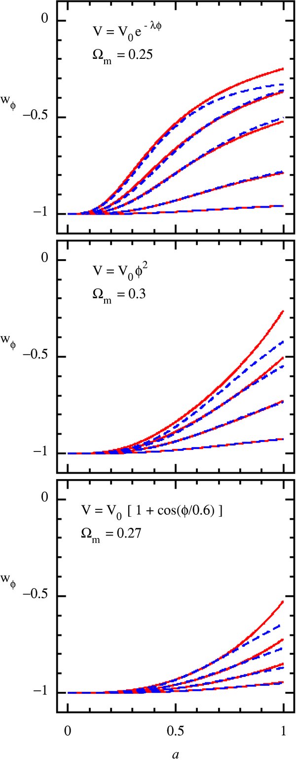
Figure 3. Examples of thawing models. The solid red lines are numerical solutions of wϕ. The dashed blue lines are calculated using the three-parameter w(a) formula (27). See the text for more details.
Download figure:
Standard image High-resolution imageIn Figure 4, we demonstrate how the parameter ζs improves our parameterization to sub-percent level. In the slow-roll regime, the ζs correction is small, and both the two- and three-parameter formulae can fit the numerical solution well. But the ζs correction becomes important in the moderate-roll regime.

Figure 4. Example showing how the ζs parameter improves our parameterization in the moderate-roll case. The solid red lines are numerical solutions of wϕ. The dashed blue lines are w(a) trajectories calculated with the three-parameter ansatz (Equation (27)). The dotted green lines are two-parameter approximations obtained by forcing ζs = 0.
Download figure:
Standard image High-resolution imageThe last example, shown in Figure 5, is a phantom model.

Figure 5. Example of the phantom model. The solid red lines are numerical solutions of wϕ. The dashed blue lines are w(a) trajectories calculated with the three-parameter w(a) formula (27).
Download figure:
Standard image High-resolution image4. OBSERVATIONAL CONSTRAINTS
In this section, we compile the updated cosmological data sets and use them to constrain the quintessence and phantom models.
4.1. Current Data Sets Used
For each of the data sets used in this paper we either wrote a new module to calculate the likelihood or modified the CosmoMC likelihood code to include dynamic w models.
Cosmic microwave background. Our complete CMB data sets include WMAP 7 yr (Komatsu et al. 2010; Jarosik et al. 2010), ACT (The ACT Collaboration et al. 2010), BICEP (Chiang et al. 2010), QUaD (Castro et al. 2009), ACBAR (Reichardt et al. 2009; Kuo et al. 2007; Runyan et al. 2003; Goldstein et al. 2003), CBI (Sievers et al. 2007; Readhead et al. 2004a, 2004b; Pearson et al. 2003), BOOMERANG (Jones et al. 2006; Piacentini et al. 2006; Montroy et al. 2006), VSA (Dickinson et al. 2004), and MAXIMA (Hanany et al. 2000).
For high-resolution CMB experiments we need to take account of other sources of power beyond the primary CMB. We always include the CMB lensing contribution even though with current data its influence is not yet strongly detected (Reichardt et al. 2009). For most high-resolution data sets, radio sources have been subtracted and residual contributions have been marginalized over (The ACT Collaboration et al. 2010). However, other frequency-dependent sources will be lurking in the data, and they too should be marginalized over. We follow a well-worn path for treating the thermal Sunyaev–Zeldovich (SZ) secondary anisotropy (Sunyaev & Zeldovich 1972, 1980): we use a power template from a gas dynamical cosmological simulation (with heating only due to shocks) described in Bond et al. (2002, 2005) with an overall amplitude multiplier ASZ, as was used in the CBI and ACBAR papers. This template does not differ by much from the more sophisticated ones obtained by Battaglia et al. (2010) that include cooling and feedback. Other SZ template choices with different shapes and amplitudes (Komatsu & Seljak 2002; Sehgal et al. 2010) have been made by the Wilkinson Microwave Anisotropy Probe (WMAP) and ACT and SPT, and as a robustness alternative by CBI. A key result is that as long as the "nuisance parameter" ASZ is marginalized, other cosmological parameters do not vary much as the SZ template changes. We make no other use of ASZ here, although it can encode the tension between the cosmology derived from the CMB primary anisotropy and the predictions for the SZ signal in that cosmology.
In addition to thermal SZ, there are a number of other sources: kinetic SZ with a power spectrum whose shape roughly looks like the thermal SZ one (Battaglia et al. 2010); and submillimeter dusty galaxy sources, which have clustering contributions in addition to Poisson fluctuations. Thermal SZ is a small effect at WMAP and Boomerang resolution. At CBI's 30 GHz, kinetic SZ is small compared with thermal SZ, but it is competitive at ACBAR, QUaD's, and ACT's 150 GHz and of course dominates at the ∼220 GHz thermal-SZ null, but the data are such that little would be added by separately modeling the frequency dependence and shape difference of it, so de facto it is bundled into the generic ASZ of the frequency-scaled thermal-SZ template. We chose not to include the SPT data in our treatment because the influence of the submillimeter dusty galaxy sources should be simultaneously modeled, and where its band powers lie (beyond ℓ ∼ 2000), the primary SZ power is small.
Type Ia supernova. We use the Kessler et al. (2009) data set, which combines the SDSS-II SN samples with the data from the ESSENCE project (Miknaitis et al. 2007; Wood-Vasey et al. 2007), the Supernova Legacy Survey (SNLS; Astier et al. 2006), the Hubble Space Telescope (HST; Garnavich et al. 1998; Knop et al. 2003; Riess et al. 2004, 2007), and a compilation of nearby SN measurements. Two light curve fitting methods, MLCS2K2 and SALT-II, are employed in Kessler et al. (2009). The different assumptions about the nature of the SN color variation lead to a significant apparent discrepancy in w. For definiteness, we choose the SALT-II-fit results in this paper, but caution that if we had tried to assign a systematic error to account for the differences in the two methods the error bars we obtain would open up, and the mean values for 1 + w may not center as much around zero as we find.
Large-scale structure. The LSS data are for the power spectrum of the Sloan Digital Sky Survey Data Release 7 (SDSS-DR7) Luminous Red Galaxy (LRG) samples (Reid et al. 2010). We have modified the original LSS likelihood module to make it compatible with time-varying w models.
Weak lensing. Five WL data sets are used in this paper. The effective survey area and galaxy number density of each survey are listed in Table 1.


Table 1. Weak Lensing Data Sets
| Data Sets | (deg2) | neff (arcmin−2) |
|---|---|---|
| COSMOSa | 1.6 | 40 |
| CFHTLS-wideb | 22 | 12 |
| GaBODSc | 13 | 12.5 |
| RCSd | 53 | 8 |
| VIRMOS-DESCARTe | 8.5 | 15 |

Notes. aMassey et al. (2007); Lesgourgues et al. (2007). bHoekstra et al. (2006); Schimd et al. (2007). cHoekstra et al. (2002); Hoekstra et al. (2002). dHoekstra et al. (2002); Hoekstra et al. (2002). eVan Waerbeke et al. (2005); Schimd et al. (2007).
Download table as: ASCIITypeset image
For the COSMOS data, we use the CosmoMC plug-in written by Lesgourgues et al. (2007) with our modifications for dynamic DE models.
For the other four WL data sets we use the covariance matrices given by Benjamin et al. (2007). To calculate the likelihood we wrote a CosmoMC plug-in code. We take the best-fit parameters α, β, z0 for n(z) ∝ (z/z0)αexp [ − (z/z0)β], and marginalize over z0, assuming a Gaussian prior with a width such that the mean redshift zm has an uncertainty of 0.03(1 + zm). We have checked that further marginalizing over other n(z) parameters (α and β) has no significant impact (DeLope Amigo et al. 2009).
Lyα forest. Two Lyα data sets are applied: (1) the set from Viel et al. (2004) consisting of the LUQAS sample (Kim et al. 2004) and the data given in Croft et al. (2002), and (2) the SDSS Lyα data presented in McDonald et al. (2005) and McDonald et al. (2006). To calculate the likelihood we interpolate the χ2 table in a three-dimensional parameter space, where the three parameters are amplitude, index, and the running of linear CDM power spectrum at pivot k = 0.9 h Mpc−1.
Other constraints. We have also used in CosmoMC the following observational constraints: (1) the distance-ladder constraint on Hubble parameter, obtained by the HST Key Project (Riess et al. 2009); (2) constraints from the BBN: Ωb0h2 = 0.022 ± 0.002 (Gaussian prior) and ΩΛ(z = 1010) < 0.2 (see Steigman 2006; O'Meara et al. 2006; Ferreira & Joyce 1997; Bean et al. 2001; Copeland et al. 2006); and (3) an isotopic constraint on the age of universe 10Gyr < age < 20Gyr (see e.g., Dauphas 2005). For the combined data sets, none of these add much. They are useful if we are looking at the impact of the various data sets in isolation on constraining our parameters.
4.2. CosmoMC Results for Current Data
Using our modified CosmoMC, we ran Markov Chain Monte Carlo (MCMC) calculations to determine the likelihood of cosmological parameters, which include the standard six, ASZ and our DE parameters, w0–wa, for Figure 1 and the new ones εs, |εϕ∞|/m, and ζs for most of the rest. Here we use |εϕ∞|/m as a fundamental parameter to eliminate the dependence of εϕ∞ on m and the sign of εs, whereas εϕ∞ adjusts as one evolves from a relativistic to non-relativistic matter EOS. The main results are summarized in Table 2. The basic six are Ωb0h2, proportional to the current physical density of baryons; Ωc0h2, the physical cold dark matter density; θ, the angle subtended by sound horizon at "last scattering" of the CMB, at z ∼ 1100; ln As, with As being the primordial scalar metric perturbation power evaluated at pivot wavenumber k = 0.002 Mpc−1; ns, the spectral index of primordial scalar metric perturbation; and τ, the reionization Compton depth. The measures on each of these variables are taken to be uniform. Derived parameters include zre, the reionization redshift; age (Gyr), the age of universe in units of gigayears; σ8, today's amplitude of the linear-extrapolated matter density perturbations over a top-hat spherical window with radius 8 h−1 Mpc. And, of great importance for DE, Ωm0; and H0 in unit of km s−1Mpc−1, which set the overall energy scale of late inflatons.
Table 2. Cosmic Parameter Constraints: ΛCDM, w0-CDM, w0–wa-CDM, εs–εϕ∞–ζs-CDM
| ΛCDM | w = w0 | w=w0+wa(1 − a) | Track+Thaw | Thaw | |
|---|---|---|---|---|---|
| Current data: CMB+LSS+WL+SN1a+Lyα | |||||
| Ωb0h2 | 0.0225+0.0004−0.0004 | 0.0225+0.0004−0.0004 | 0.0225+0.0004−0.0004 | 0.0225+0.0004−0.0004 | 0.0225+0.0004−0.0004 |
| Ωc0h2 | 0.1173+0.0020−0.0019 | 0.1172+0.0024−0.0024 | 0.1177+0.0025−0.0023 | 0.1174+0.0029−0.0029 | 0.1175+0.0023−0.0022 |
| θ | 1.042+0.002−0.002 | 1.042+0.002−0.002 | 1.042+0.003−0.002 | 1.042+0.003−0.002 | 1.0417+0.0021−0.0021 |
| τ | 0.089+0.014−0.013 | 0.090+0.015−0.014 | 0.088+0.014−0.013 | 0.090+0.015−0.014 | 0.088+0.015−0.014 |
| ns | 0.96+0.01−0.01 | 0.96+0.01−0.01 | 0.96+0.01−0.01 | 0.96+0.01−0.01 | 0.958+0.011−0.011 |
| ln(1010As) | 3.24+0.03−0.03 | 3.24+0.03−0.03 | 3.24+0.03−0.03 | 3.24+0.03−0.03 | 3.239+0.033−0.033 |
| 0.56+0.11−0.15 | 0.56+0.11−0.14 | 0.57+0.11−0.14 | 0.56+0.11−0.14 | 0.56+0.11−0.14 | |
| Ωm | 0.292+0.011−0.010 | 0.294+0.012−0.012 | 0.293+0.012−0.012 | 0.293+0.015−0.014 | 0.293+0.013−0.011 |
| σ8 | 0.844+0.015−0.016 | 0.841+0.026−0.026 | 0.847+0.026−0.026 | 0.844+0.035−0.036 | 0.844+0.024−0.023 |
| zre | 10.8+1.2−1.1 | 10.9+1.2−1.2 | 10.7+1.1−1.1 | 10.9+1.2−1.2 | 10.8+1.2−1.2 |
| H0 | 69.2+1.0−1.0 | 69.0+1.4−1.4 | 69.2+1.4−1.4 | 69.0+1.9−1.8 | 69.1+1.4−1.4 |
| w0 | ... | −0.99+0.05−0.06 | −0.98+0.14−0.11 | ... | ... |
| wa | ... | ... | −0.05+0.35−0.58 | ... | ... |
| εs | ... | ... | ... | 0.00+0.18−0.17 | −0.00+0.27−0.29 |
| |εϕ∞|/m |
... | ... | ... | 0.00+0.21+0.58 | ... |
| ζs | ... | ... | ... | n.c. | n.c. |
| Forecasted data: Planck2.5yr + low-z-BOSS + CHIME + Euclid-WL + JDEM-SN | |||||
| Ωb0h2 | 0.02200+0.00007−0.00007 | 0.02200+0.00007−0.00007 | 0.02200+0.00007−0.00008 | 0.02200+0.00007−0.00008 | 0.02200+0.0007−0.0007 |
| Ωc0h2 | 0.11282+0.00024−0.00023 | 0.11280+0.00027−0.00027 | 0.11282+0.00026−0.00029 | 0.1128+0.0003−0.0003 | 0.1128+0.0003−0.003 |
| θ | 1.0463+0.0002−0.0002 | 1.0463+0.0002−0.0002 | 1.0463+0.0003−0.0002 | 1.0463+0.0002−0.0002 | 1.0463+0.0002−0.0002 |
| τ | 0.090+0.003−0.003 | 0.090+0.004−0.004 | 0.090+0.004−0.004 | 0.090+0.005−0.005 | 0.090+0.004−0.004 |
| ns | 0.970+0.002−0.002 | 0.970+0.002−0.002 | 0.970+0.002−0.002 | 0.970+0.002−0.002 | 0.970+0.002−0.002 |
| ln(1010As) | 3.115+0.008−0.008 | 3.115+0.009−0.009 | 3.115+0.009−0.009 | 3.115+0.010−0.010 | 3.115+0.009−0.009 |
| Ωm | 0.260+0.001−0.001 | 0.261+0.002−0.002 | 0.260+0.003−0.003 | 0.2609+0.0022−0.0022 | 0.2605+0.0027−0.0024 |
| σ8 | 0.7999+0.0016−0.0017 | 0.7994+0.0023−0.0025 | 0.800+0.003−0.003 | 0.7992+0.0027−0.0027 | 0.7996+0.0026−0.0029 |
| zre | 10.9+0.3−0.3 | 10.9+0.3−0.3 | 10.9+0.3−0.3 | 10.9+0.4−0.4 | 10.9+0.3−0.3 |
| H0 | 72.0+0.1−0.1 | 71.9+0.3−0.3 | 72.0+0.4−0.4 | 71.85+0.37−0.29 | 71.94+0.34−0.36 |
| w0 | ... | −1.00+0.01−0.01 | −1.00+0.03−0.03 | ... | ... |
| wa | ... | ... | 0.01+0.08−0.08 | ... | ... |
| εs | ... | ... | ... | 0.005+0.031−0.025 | 0.008+0.056−0.054 |
| |εϕ∞|/m |
... | ... | ... | 0.000+0.034+0.093 | ... |
| ζs | ... | ... | ... | n.c. | n.c. |

Notes. Tracking + thawing models use wde(a|εs, εϕ∞, ζs) of Equation (27). Thawing enforces εϕ∞ = 0. n.c. stands for "not constrained." H0 has units km s−1Mpc−1. θ is in radians/100. m is 3/2 (or 2) in the matter-dominated (or radiation-dominated) regime. All bounds are marginalized 1σ (68.3% CL) limits, except that for |εϕ∞|/m marginalized 1σ and 2σ (95% CL) upper bounds are given.
Download table as: ASCIITypeset image
We begin with our versions of the familiar contour plots that show how the various data sets combine to limit the size of the allowed parameter regions. Figures 6 and 7 show the best-fit cosmological parameters do depend on the specific subset of the data that is used. We find that most cosmological parameters are stable when we vary the choice of data sets. The data making the largest differences are the SDSS-DR7-LRG data driving Ωm up and the Lyα data driving σ8 up. We take SN+CMB as a "basis," for which Ωm0 = 0.267+0.019−0.018 and σ8 = 0.817+0.023−0.021. Adding LSS pushes Ωm0 to 0.292+0.011−0.010; whether or not WL and Lyα are added or not is not that relevant, as Figure 6 shows. Lyα pushes σ8 to 0.844+0.015−0.016. These drifts of best-fit values are at the ∼2σ, level in terms of the σ's derived from using all of the data sets, as is evident visually in Figure 6.

Figure 6. Marginalized 68.3% CL and 95.4% CL constraints on σ8 and Ωm0 for the ΛCDM model vary with different choices of data sets. For each data set an HST constraint on H0 and BBN constraint on Ωb0h2 have been used.
Download figure:
Standard image High-resolution image
Figure 7. Marginalized 68.3% CL and 95.4% CL constraints on εs and Ωm0, using different (combinations) of data sets. This is the key DE plot for late-inflaton models of energy scale, encoded by 1 − Ωm0 and potential gradient defining the roll-down rate, .

Download figure:
Standard image High-resolution imageFigure 7 shows how the combination of complementary data sets constrains εs and Ωm0, the two key parameters that determine low-redshift observables. The label "All" refers to all the data sets described in this section, and "CMB" refers to all CMB data sets, and so forth. In Figure 8, marginalized two-dimensional likelihood contours are shown for all our DE parameters. The left panel shows that the slope parameter εs and tracking parameter εϕ∞ are both constrained. The constraint on εs limits how steep the potential could be at low redshift. The upper bound of εϕ∞ indicates that the field cannot be rolling too fast at intermediate redshift z ∼ 1. The right panel shows that ζs is not constrained and is almost uncorrelated with εs. This is because the current observational data favor slow-roll (|1 + wϕ| ≪ 1), in which case the ζs correction in wϕ is very small. Another way to interpret this is that a slowly rolling field does not "feel" the curvature of potential. In Section 6, we will discuss the meaning and measurement of ζs in more detail.

Figure 8. Marginalized two-dimensional likelihood contours for our three DE parameters derived using "ALL" current observational data. The inner and outer contours are 68.3% CL and 95.4% CL contours. (We actually show |εϕ∞|/m since that is the attractor whether one is in the relativistic m = 2 or non-relativistic m = 3/2 regime.)
Download figure:
Standard image High-resolution imageBecause of the correlation between εs and εϕ∞, the marginalized likelihood of εs depends on the prior of εϕ∞. On the other hand, the constraint on εs will also depend on the prior on εs itself. For example, we can apply a flat prior on , rather than a flat prior on the squared slope εs. Other priors we have tried are the "thawing prior" εϕ∞ = 0, the "quintessence prior" εs>0, and "slow-roll thawing prior" εϕ∞ = ζs = 0. The results are summarized in Table 3.

Table 3. Marginalized 68.3%, 95.4%, and 99.7% CL Constraints on εs under Different Prior Assumptions
| Prior | Constraint |
|---|---|
| Flat prior on εs | εs = 0.00+0.18+0.39+0.72−0.17−0.44−0.82 |
| Flat prior on | εs = 0.00+0.09+0.27+0.46−0.07−0.28−0.52 |
| Thawing prior εϕ∞ = 0 | εs = 0.00 + 0.27+0.53+0.80−0.29−0.61−0.98 |
| Slow-roll thawing εϕ∞ = ζs = 0 | εs = −0.01+0.26+0.50+0.70−0.28−0.59−0.86 |
| Quintessence εs>0 | εs = 0.00+0.18+0.39+0.76 |

Download table as: ASCIITypeset image
In Figure 9, we show the reconstructed trajectories of the DE EOS, Hubble parameter, distance moduli, and the growth factor D of linear perturbations. The wϕ information has also been compressed into a few bands with errors, although that is only to guide the eye. The off-diagonal correlation matrix elements between bands is large, encoding the coherent nature of the trajectories. Also, the likelihood surface in all wϕ bands is decidedly non-Gaussian, and should be characterized for this information to be statistically useful in constraining models by itself. The other variables shown involve integrals of wϕ, and thus are not as sensitive to detailed rapid change aspects of wϕ, which, in any case, our late-inflaton models do not give. The bottom panels show how impressive the constraints on trajectory bundles should become with planned experiments, a subject to which we now turn.

Figure 9. Best-fit trajectory (heavy curve) and a sample of trajectories that are within 1σ (68.3% CL). In the upper panels the current data sets are used, and lower panels the forecast mock data. From left to right the trajectories are the DE EOS, the Hubble parameter rescaled with H−10(1 + z)3/2, the distance moduli with a reference ΛCDM model subtracted, and the growth factor of linear perturbation rescaled with a factor (1 + z) (normalized to be unit in the matter-dominated regime). The current SN data are plotted against the reconstructed trajectories of distance moduli. The error bars shown in the upper left and lower left panels are 1σ uncertainties of 1 + w in bands 0 < a ⩽ 0.25, 0.25 < a ⩽ 0.5, 0.5 < a ⩽ 0.75, and 0.75 < a ⩽ 1.
Download figure:
Standard image High-resolution image5. FUTURE DATA FORECASTS
In this section, we discuss the prospects for further constraining the parameters of the new w(a) parameterization using a series of forthcoming or proposed cosmological observations: from the Planck satellite CMB mission (Tauber 2005; Clavel & Tauber 2005; Planck Science Team 2009), from a JDEM (Joint Dark Energy Mission; Albrecht et al. 2006) for SNIa observations, from a WL survey by the Euclid satellite (Euclid Study Team 2009), and from future BAO data that could be obtained by combining low-redshift galaxy surveys with a redshifted 21 cm survey of moderate z ∼ 2. The low-redshift galaxy surveys for BAO information can be achieved by combining a series of ground-based galaxy observations, such as Baryon Oscillation Spectroscopic Survey (BOSS; Schlegel et al. 2007). For the 21 cm survey, we assume a 200 m × 200 m ground-based cylinder radio telescope (Chang et al. 2008; Peterson et al. 2009; Morales & Wyithe 2010), which is the prototype of the proposed experiment CHIME (Canadian Hydrogen Intensity Mapping Experiment). Unless specified, we use the fiducial model in Table 4 to simulate the mock data sets.
Table 4. Fiducial Model used in Future Data Forecasts
| Ωb0h2 | Ωc0h2 | h | σ8 | ns | τ |
|---|---|---|---|---|---|
| 0.022 | 0.1128 | 0.72 | 0.8 | 0.97 | 0.09 |
Download table as: ASCIITypeset image
5.1. The Mock Data Sets
5.1.1. Planck CMB Simulation
Planck 2.5 years (five sky surveys) of multiple (CMB) channel data are used in the forecast, with the instrument characteristics for the channels used listed in Table 5 using Planck "Blue Book" detector sensitivities and the values given for the full width half-maxima (FWHMs).
Table 5. Planck Instrument Characteristics
| Channel Frequency (GHz) | 70 | 100 | 143 |
|---|---|---|---|
| Resolutiona (arcmin) | 14 | 10 | 7.1 |
| Sensitivityb intensity (μK) | 8.8 | 4.7 | 4.1 |
| Sensitivity polarization (μK) | 12.5 | 7.5 | 7.8 |
Notes. aFWHM assuming Gaussian beams. bThis is for 30 months of integration.
Download table as: ASCIITypeset image
For a nearly full-sky (we use fsky = 0.75) CMB experiment, the likelihood can be approximated with the following formula (Baumann et al. 2009):


where lmin = 3 and lmax = 2500 have been used in our calculation. Here, is the observed (or simulated input) angular power spectrum and Cl is the theoretical power spectrum plus noise.

We use the model described in Dunkley et al. (2009) and Baumann et al. (2009) to propagate the effect of polarization foreground residuals into the estimated uncertainties on the cosmological parameters. For simplicity, only the dominating components in the frequency bands we are using, i.e., the synchrotron and dust signals, are considered in our simulation. The fraction of the residual power spectra are all assumed to be 5%.
5.1.2. JDEM SN Simulation
For the JDEM SN simulation, we use the model given by the DETF forecast (Albrecht et al. 2006), with roughly 2500 spectroscopic SN at 0.03 < z < 1.7 and 500 nearby samples. The apparent magnitude of SN is modeled as

where δnear is unity for the nearby samples and zero otherwise.
There are four nuisance parameters in this model. The SN absolute magnitude is expanded as a quadratic function M − μLz − μQz2 to account for the possible redshift dependence of the SN peak luminosity, where M is a free parameter with a flat prior over −∞ < M < +∞; and for μL and μQ, Gaussian priors (the "pessimistic" case in the DETF forecast) are applied. Finally, given that the nearby samples are obtained from different projects, an offset μS is added to the nearby samples only. For μS we apply a Gaussian prior μS = 0.00 ± 0.01.

The intrinsic uncertainty in the SN absolute magnitude is assumed to be 0.1, to which an uncertainty due to a peculiar velocity 400 km s−1 is quadratically added.
5.1.3. BAO Simulation
The "Baryon Acoustic Oscillations" (BAO) information can be obtained by combining a series of ground-based low-redshift galaxy surveys with a high-redshift 21 cm survey. We assume a fiducial galaxy survey with comoving galaxy number density 0.003 h3 Mpc−3 and sky coverage 20,000 deg2, which is slightly beyond, but not qualitatively different from the specification of the SDSS-III BOSS project. The 21 cm BAO survey using a ground-based cylinder radio telescope has been studied by Chang et al. (2008), Peterson et al. (2009), and Seo et al. (2010). The specifications we have used are listed in Table 6.
Table 6. 21 cm BAO Survey Specifications
| Parameter | Specification |
|---|---|
| Shot noise | 0.01h3 Mpc−3 |
| Survey area | 15,000 deg2 |
| Number of receivers | 4000 |
| Integration time | 4 years |
| Cylinder telescope | 200 m ×200 m |
| Antenna temperature | 50K |
| Bias | 1 |
Download table as: ASCIITypeset image
For more details about the BAO forecast technique, the reader is referred to Seo & Eisenstein (2007) and Seo et al. (2010).
5.1.4. EUCLID Weak Lensing Simulation
We assume a WL survey with the following "Yellow Book" EUCLID specifications (Euclid Study Team 2009):

where 〈γ2int〉1/2 is the intrinsic galaxy ellipticity, and is the average galaxy number density being observed. At high ℓ, the non-Gaussianity of the dark matter density field becomes important (Doré et al. 2009). For simplicity we use an ℓ-cutoff ℓmax = 2500 to avoid modeling the high-ℓ non-Gaussianity, which will provide more cosmic information, hence, the WL constraints shown in this paper are conservative.

We use a fiducial galaxy distribution,

The galaxies are divided into four tomography bins, with the same number of galaxies in each redshift bin. The uncertainty in the median redshift in each redshift bin is assumed to be 0.004(1 + zm), where zm is the median redshift in that bin.
In the ideal case in which the galaxy redshift distribution function is perfectly known, the formula for calculating WL tomography observables and covariance matrices can be found in, e.g., Ma et al. (2006). In order to propagate the uncertainties of photo-z parameters onto the uncertainties of the cosmological parameters, we ran Monte Carlo simulations (with random Gaussian shift of the median redshift in each bin) to obtain the covariance matrices due to redshift uncertainties, which are then added to the ideal covariance matrices.
5.2. Results of the Forecasts
The constraints on cosmological parameters from future experiments are shown in Table 2 below those for current data. The future observations should improve the measurement of εs significantly—about five times better than the current best constraint. There is also a significant improvement on the upper bound of εϕ∞, which together with the constraint on εs can be used to rule out many tracking models. The running parameter ζs remains unconstrained.
To compare different DE probes, in Figure 10 we plot the marginalized constraints on Ωm0 and εs for different data sets. To break the degeneracy between DE parameters and other cosmological parameters, we apply the Planck-only CMB constraints as a prior on each of the non-CMB data sets.

Figure 10. Marginalized two-dimensional likelihood contours. Using mock data and assuming thawing prior (εϕ∞ = 0), the inner and outer contours of each color correspond to 68.3% CL and 95.4% CL, respectively. See the text for more details.
Download figure:
Standard image High-resolution imageThe forecasted BAO, WL, and SN results, when combined with the Planck prior, are all comparable. We note in particular that the ground-based BAO surveys deliver similar measurements at a fraction of the cost of the space experiments, although of course much useful collateral information will come from all of the probes.
The shrinkage in the allowed parameter space is visualized in Figure 9 through the decrease in area of the trajectory bundles from current to future data, showing trajectories of 1 + wϕ sampled down to the 1σ level. We also show the mean and standard deviation of 1 + wϕ at the center of four uniform bands in a. As mentioned above, the bands are highly correlated because of the coherence of the trajectories, a consequence of their physical origin. We apply such band analyses to early (as well as late) universe inflation that encodes such smoothing theory priors in future papers.
Figure 9 also plots trajectories, which are flat in the high-redshift matter-dominated regime. They are less spread out than the w bundle because H depends upon an integral of w. One of the observable quantities measured with SNe is the luminosity distance. What we plot is something more akin to relative magnitudes of standard candles, 5log10(dL/dL;ref), in terms of dL;ref, the luminosity distance of a reference ΛCDM model. For luminosity distance trajectories reconstructed with the current data we choose a reference model with Ωm0 = 0.29, which the SDSS LSS data drove us to; for forecasts, we chose Ωm0 = 0.26, what the other current data are more compatible with, for the reference. Because the SN data only measure the ratio of luminosity distances, for each trajectory we normalize dL/dL;ref to be unit in the low-redshift limit by varying H0 in the reference model. The error bars shown are for the current SN data (Kessler et al. 2009), showing compatibility with ΛCDM, and, based upon the coherence of the quintessence-based prior and the large error bars, little flexibility in trying to fit the rise and fall of the data means.

The rightmost panels of Figure 9 show the linear growth factor for dark matter fluctuations relative to the expansion factor, (1 + z)D(z). The normalization is such that it is unity in the matter-dominated regime. It should be determined quite precisely for the quintessence prior with future data.
6. DISCUSSION AND CONCLUSIONS
6.1. Slow-roll Thawing Models, Their One-parameter Approximation, and the Burn-in to It
In slow-roll thawing models, to first order w(z) only depends on two physical quantities: one determining "when to roll down," quantified mostly by 1 − Ωm0, and one determining "how fast to roll down," quantified by the slope of the potential, i.e., εs, since εϕ∞ = 0, and ζs ≈ 0:

where F is an analytical function given by Equation (25), and to sufficient accuracy. We plot F2(x) in the left panel of Figure 11. It is zero in the small a regime and unity in the large a regime, and at aeq is . The right panel of Figure 11 plots the derivative dF2/dx showing |dw/da| maximizes around a = aeq (at redshift ∼0.4). A few examples of 1 + w(a) are plotted in Figure 12 to show the mapping from εs to w(a) trajectories. Three stages are evident in the significant time dependence of dw/da: the Hubble-frozen stage at a ≪ aeq, where w has the asymptotic value −1; the thawing stage when the DE density is comparable to the matter component; and the future inflationary stage where DE dominates (a ≫ aeq) and a future attractor with 1 + w → 2εs/3 is approached, agreeing with the well-known early-inflation solution 1 + w = 2V/3.
![$a_{\rm eq}\vert _{\rm slowroll, thawing} \approx (\frac{{\Omega _{m0}}}{1-{\Omega _{m0}}}) ^{1/[3-1.08(1-{\Omega _{m0}})\varepsilon _{s} ]}$](https://content.cld.iop.org/journals/0004-637X/726/2/64/revision1/apj373813ieqn59.gif)
![$F^2(1)=[\sqrt{2}-\ln (1+\sqrt{2})]^2 \approx 0.284$](https://content.cld.iop.org/journals/0004-637X/726/2/64/revision1/apj373813ieqn60.gif)

Figure 11. Left panel: the function F2(x) with x = a/aeq defined by Equation (25). Right panel: the derivative dF2/dx, showing where wϕ changes most quickly in thawing models, namely near aeq.
Download figure:
Standard image High-resolution image
Figure 12. Trajectories of 1 + w(a) for different values of εs. For all trajectories εϕ∞ and ζs are fixed to be zero, and Ωm = 0.3. From bottom to top, εs is set to be −0.75, −0.5, −0.25, 0, 0.25, 0.5, and 0.75, respectively.
Download figure:
Standard image High-resolution imageEven with such models, there is in principle another parameter: the initial field momentum is unlikely to be exactly on the εϕ∞ = 0 attractor. In that case, falls as a−3 until the attractor is reached, a "burn-in" phase. (Such burn-in phases are evident in Figure 2 for tracking models.) In early work on parameterizing late inflatons we added a parameter as to characterize when this drop toward the attractor occurred, and found it could be (marginally) constrained by the data to be small relative to the a-region over which the trajectories feel the DE-probing data. However, we decided to drop this extra parameter for this paper since the expectation of late-inflaton models is that the attractor would have been established long before the redshift range relevant for DE probes.

The three-parameter, two-parameter, and one-parameter fits all give about the same result for the statistics of εs derived from current data. Figure 13 illustrates why we find εs ≈ 0.0 ± 0.28. It shows the confrontation of banded SN data on distance moduli defined by

where dL is the physical luminosity distance, with trajectories in μ with differing values of εs (for the h (or Ωm0) values as described.) The current DE constraints are largely determined by SN, in conjunction with the Ωmh2-fixing CMB.

Figure 13. Dependence of distance moduli μ(z) on the slope parameter εs for slow-roll thawing models. The prediction of μ(z) from a reference ΛCDM model with Ωm0 = 0.29 is subtracted from each line. The SN samples are binned into redshift bins with bin width Δz = 0.3.
Download figure:
Standard image High-resolution image6.2. A w0–wa Degeneracy for the Slow-roll Thawing Model Prior
The parameterization (43) can be simply related to the phenomenological w0–wa parameterization by a first-order Taylor series expansion about a redshift zero pivot:

and

From formula (43), it follows that w0 and wa should satisfy the linear relation

where

is roughly the scale factor where the field is unfrozen. Over the range of 0.17 < Ωm < 0.5, this constraint Equation (47) can be well approximated by the formula

Such a degeneracy line is plotted in Figure 1. Rather than a single w0 parameter, constraining to this line based on a more realistic theoretical prior obviously makes for a more precise measurement of w. On the other hand, once the measurements of w0 and wa are both sufficiently accurate, the slow-roll thawing models could be falsified if they do not encompass part of the line. Obviously, though, it would be better to test deviations relative to true thawing trajectories rather than the ones fit by this perturbation expansion about redshift zero. One way to do this is to demonstrate that 1 + w∞ is not compatible with zero, as we now discuss.
Similar w0–wa relations have appeared in Kallosh et al. (2003) for the linear potential and de Putter & Linder (2008) for the pnGB model. Our thorough analytic treatment here shows that such a relation: (1) is general for all slow-roll thawing models and (2) depends on Ωm0.
6.3. Transforming w0–wa and εs–εϕ∞ Contours into w0–w∞ Contours
The DETF w0–wa parameterization which is linear in a can be thought of as a parameterization in terms of w0 and w∞ = wa + w0 (or de,0 and de,∞ in the DE acceleration factor language). The upper panel w0–wa contour map in Figure 14 shows that it is only a minor adjustment of the w0–wa of Figure 1. If we said there is a strict dichotomy between trajectories that are quintessence and trajectories that are phantom, as has been the case in our treatment in this paper, only the two of the four quadrants of Figure 14 would be allowed. (In the w0–wa figures, the prior looks quite curious visually, in that the line wa = −(1 + w0) through the origin has only the region above it allowed in the 1 + w0>0 regime, and only the region below it allowed in the 1 + w0 < 0 regime.)

Figure 14. Upper panel shows the marginalized 68.3% (inner contour) and 95.4% (outer contour) constraints on w0 and w∞ for the conventional linear DETF parameterization, recast as w = w∞ + (w0 − w∞)a, using the current data sets described in Section 4. It is a slightly tilted version of the w0–wa version in Figure 1. The demarcation lines transform to just the two axes, with the upper right quadrant the pure quintessence regime, and the lower right quadrant the pure phantom regime. If the cross-over of partly phantom and partly quintessence are excluded, as they are for our late-inflaton treatment in this paper, the result looks similar to the lower panel, in which the two-parameter εs-εϕ∞ formula has been recast into 2ε0/3 and 2ε∞/3, via . However, as well the prior measure has also been transformed, from our standard uniform dεsdεϕ∞ one to a uniform dε0dεϕ∞ one. The quadrant exclusions are automatically included in our re-parameterization.

Download figure:
Standard image High-resolution imageTo make this issue more concrete, we show in the lower panel of Figure 14 what happens for our physics-motivated two-parameter linear model, Equation (33), except that it is linear for , and in the "time variable" F not in a. In terms of wϕ0 and wϕ∞, we have [1 − F(a/aeq)/F(1/aeq)]. The prior measure on 1 + wϕ0 and wϕ∞ is uniform as in the linear-a case. Once the prior that only two quadrants are allowed is imposed upon the linear-a case, it looks reasonably similar to the lower panel.


The determination of our various parameters depends upon an extended redshift regime with direct or indirect observational information. An error in a parameter is built up by a sum of deviations of the observational data from the observable constructed using the model for wde, using the maximum likelihood formula. The data-sensitive redshift regime is quite extended, not concentrated around zero redshift for w0, not concentrated at high redshift for w∞ or εϕ∞, and not concentrated at aeq for εs. An illustration of the redshift reach of the εs parameter is Figure 13 for the SN observable, namely a magnitude difference. The specific redshift reach is very data dependent of course.
6.4. ζs, the Potential Curvature, and the Difficulty of Reconstructing V(ϕ)
For slow-roll thawing quintessence models, the running parameter ζs can be related to the second derivative of ln V. Using the single-parameter approximation we can approximately calculate dϕ/dln a at a = aeq. The result is

An immediate consequence is that the amount that ϕ rolls, at least at late time, is small compared with the Planck mass. In the slow-roll limit, to the zeroth order, Equation (26) can be reformulated as

Combining Equations (50) and (51), and that , we obtain


where

For phantom models C is negative.
We have shown in Section 5 that, for the fiducial ΛCDM model (with εs = εϕ∞ = 0), the running parameter ζs cannot be measured. For a nearly flat potential, the field momentum is constrained to be very small, hence so is the change δϕ, so the second-order derivative of ln V is not probed. To demonstrate what it takes to probe ζs, we ran simulations of fiducial models with varying εs (0, 0.25, 0.5, and 0.75). The resulting forecasts for the constraints on εs and ζs are shown in Figure 15. We conclude that unless the true model has a large εs ≳ 0.5, which is disfavored by current observations at nearly the 2σ level, we will not be able to measure ζs. Thus if the second derivative of ln V is of order unity or less over the observable range, as it has been engineered to be in most quintessence models, its actual value will not be measurable. However, if |Mp2d2ln V/dϕ2| ≫ 1, the field would be oscillating. Though in their own right, oscillatory quintessence models are not considered in this work.

Figure 15. 68.3% CL (inner contours) and 95.4% (outer contours) CL constraints on εs and ζs, using forecasted CMB, WL, BAO, and SN data. The thawing prior (εϕ∞ = 0) has been used to break the degeneracy between εs and εϕ∞. The four input fiducial models labeled with red points have ζs = 0 and, from bottom to top, εs = 0, 0.25, 0.5, and 0.75, respectively. Only for large gradients can ζs be measured and a reasonable stab at potential reconstruction be made.
Download figure:
Standard image High-resolution image6.5. Field Momentum and the Tracking Parameter εϕ∞
The late-universe acceleration requires the field to be in a slow-roll or at most a moderate-roll at low redshift. In tracking models, the high redshift ϕ constancy implies the kinetic energy density follows the potential energy density of the scalar field: Π2ϕ/2V → εϕ∞/(3 − εϕ∞). The field could be fast-rolling in the early universe, with large εϕ∞ and a steep potential, and indeed is the case for many tracking models. If the potential is very flat, field momenta fall as a−3, The rate of Hubble damping in the flat potential limit is . However, as proposed in most tracking models, the potential is steep at high redshift, and gradually turns flat at low redshift. The actual damping rate itself is related to the field momentum, which again relies on how steep potential is at high redshift. The complicated self-regulated damping behavior of field momentum is encoded in the tracking parameter εϕ∞ in Equation (27) (see Figure 16 where the damping of field momentum is visualized in w(z) space). At high redshift the approximation completely fails, but at low redshift the damping rate asymptotically approaches sxs .


Figure 16. Dependence of wϕ(z) on εϕ∞ and ζs. We have fixed Ωm0 = 0.27 and εs = 0.5. The red solid lines correspond to ζs = 0, green dashed lines ζs = −0.5, and blue dotted lines ζs = 0.5. For each fixed ζs, the lines from bottom to top correspond to |εϕ∞|/m = 0, 0.3, 0.6, and 0.9.
Download figure:
Standard image High-resolution imageSince DE is subdominant at high redshift, the observational probes there are not very constraining. In the three-parameter approximation, instead of an asymptotic εϕ∞, we could use a moderate redshift pivot zpivot ∼ 1, with variables , εs, and ζs, and the asymptotic regime now a controlled extrapolation. Indeed, using the method of Section 6.3 we could define everything in terms of pivots of ϕ; for example, at z = 0 as we used in Section 6.3, and with a third about half way in between 0 and 1, such as at aeq, which is about 0.7, so zeq ∼ 0.4. Since all would be functions of our original three parameters and aeq through the specific evaluations of F and F2 at the pivots, the formula does not change, but the measure (prior on the parameters) would be different, namely to one uniform in the three s.


Whatever the specific parameters chosen, in all cases the lack of high-redshift constraining power means that our reconstructed wϕ(a) trajectories such as in Figure 9 should be regarded as low-redshift observational constraints extrapolated through theory-imposed priors on the smooth change in quintessence paths at high redshift. The tracking assumption that we have used in this paper provides one such extrapolation, but others may be considered. For these, we need to define a prior on and information on the damping rate of , and this could have an impact on the marginalized posterior likelihood of εs. We have presented an example of this, showing that whereas the flat prior 0 ⩽ |εϕ∞| < m gives εs = 0.00+0.18−0.17, the εϕ∞ = 0 "thawing prior" gives εs = −0.00+0.27−0.29. We note though that because DE is so subdominant at higher redshift, observables such as the Hubble parameter H(z), the luminosity distance dL(z), and the linear perturbation growth rate D(z) are insensitive to the high-z extrapolation of wϕ(z), as we showed in Figure 9. Thus, even for the SUGRA model shown in the middle panel of Figure 2 with a time-varying attractor which is not fit as well at high z, what the data say about it is confined to low z, and hence the results obtained with our formula apply to such models as well; in particular, the late-time potential steepness must be controlled according to the εs constraint for them to be viable.


6.6. Using Our wϕ Parameterization
Suppose that one has in mind a specific quintessence potential V(ϕ). How can our constraints, in particular on εs, be used to test viability? The first thing is to see what V looks like at a function of ϕ. One does not know ϕeq of course, but it had better lie in the range for εs allowed by the data. The model would be ruled out if no ϕ has V penetrating the allowed region. Otherwise, the field equation of motion has to be solved to get ϕeq and hence εs from its definition. Such a calculation is inevitable because quintessence models do not solve the fine-tuning problem. For tracking models, the low-redshift dynamics is usually designed (i.e., are fine-tuned) to deviate from an attractor. For thawing models, the initial value of ϕ∞ (to which ϕ is frozen at high redshift) needs to be fine-tuned as well.
Although it seems unlikely that the community will abandon the DETF-sanctioned w0–wa linear a model and its FOM as a way to state results for current and future DE experiments, our easy-to-use εs constraint with its clear physics-based meaning could be quoted as well. The two-parameter case goes well beyond linear a with the same number of parameters. Because we learn little about the third parameter one might think that the three-parameter case has one parameter too many to bother with, but it is not really redundant since it helps to accurately pave the wϕ paths. To facilitate general-purpose use of this parameterization, we wrote a fortran90 module that calculates wϕ(a|εs, εϕ∞, ζs, Ωm0) (http://www.cita.utoronto.ca/~zqhuang/work/wphi.f90). The f90 code is well wrapped so that implementing it in CosmoMC is similar to what has to be done to install the w0–wa parameterization to deliver more physically meaningful MCMC results.
We are grateful for useful discussions with Patrick MacDonald, Andrei Frolov, and Dmitry Pogosyan.
APPENDIX: COMPARISON WITH OTHER PARAMETERIZATIONS
The constant w model and the linear w models, w = w0 + wa(1 − a) or w = w0 + w1z with a cutoff (Upadhye et al. 2005; Linder & Huterer 2005), are the simplest wde parameterizations widely used in the literature. An advantage is that they can fit many DE models, including those beyond scalar field models, at low redshifts. A disadvantage is that they fail at z ≳ 1 for most physical models, and in this high-precision cosmology era we cannot ignore adequate inclusion of the z ∼ 1 information. For this reason, there are various three-parameter or four-parameter approximations proposed to improve w at higher redshifts. Some examples are simple extensions of w0–wa.
- Replacement of (1 − a) by (1 − ab), with b being a parameter added to w0, wa (Linder & Huterer 2005),Four-parameter models include
- where w0, w1, as, p are the parameters (Hannestad & Mörtsell 2004);
- where w0, wm, ac, Δ are constants (Corasaniti & Copeland 2003);
- where wf, Δw, at, τ are the parameters (Linder & Huterer 2005).


Many of these four-parameter models describe a wϕ-transition characterized by an initial w, today's w, a transition redshift, and a duration of transition. For the tracking models they are meant to describe, such a phenomenology introduces three parameters to describe essentially one degree of freedom (the tracking attractor). Instead our parameterization consistently solves the tracking wϕ(a).
Chiba (2010) has done similar work for the negative power-law tracking models, though did not model the low-redshift slow-roll regime, making his parameterization much less useful than ours for comparing with data.
Slow-roll quintessence models have been studied by, e.g., Crittenden et al. (2007), Scherrer & Sen (2008), and Chiba (2009), but our work makes significant improvements. First, we have chosen a more optimal pivot a = aeq to expand ln V(ϕ), whereas the other works expand V(ϕ) at either a ≪ 1 or a = 1. As a result, we approximate wϕ at the sub-percent level in the slow-roll regime |1 + w| < 0.2 compared with the other approximations failing at |1 + wϕ|>0.1. Second, with the field momentum from the tracking regime incorporated, our three-parameter wϕ(a) ansatz can also fit the more extreme moderate-roll and tracking models with an accuracy of a few percent. Since current data allow a relatively large region of parameter space (|1 + wϕ| ≲ 0.2 at 99.7% CL), a slow-roll prior with |1 + wϕ| ≪ 1 should not be imposed as other papers have done. Third, we have extended the parameterization to cover phantom models, though that is arguably not a virtue.
A.1. ρde(z) and H(z) Reconstruction
One has to integrate wϕ(z) once to get the DE density ρϕ(z) and the Hubble parameter H(z). Observational data are often directly related to either H(z) or ρde(z), and not sensitive to wde(z) variations. Thus, one may prefer to directly parameterize ρde(z) (Wang & Tegmark 2004; Alam et al. 2004) or H(z) (Sahni et al. 2003; Alam et al. 2004, 2007) on phenomenological grounds. A semi-blind expansion of H(z) or ρde(z), e.g., in polynomials or in bands, differs from one in wde(z), since the prior measures on the coefficients are radically altered. By contrast, a model such as ours for wde(z; εs, εϕ∞, ζs) characterized by physical parameters is also a model for H(z; εs, εϕ∞, ζs) or ρde(z; εs, εϕ∞, ζs), obtained by integration.
Where the freedom does lie is in the prior measures imposed on the parameters, a few examples of which were discussed in Section 4.
A.2. V(ϕ) Reconstruction
For thawing models, our parameters εs and ζs are based on a local expansion of ln V(ϕ) at low redshift. One should obtain similar results by directly reconstructing the local V(ϕ). An attempt at local V(ϕ) reconstruction was done in Sahlén et al. (2005), where a polynomial expansion was used,

with ϕ chosen to be zero at present. A result highlighted in that paper is that there is a strong degeneracy between V1 and . We shall see that this degeneracy is actually a result of the prior, and not something that observational data are telling us, as we now show.

For simplicity we assume that Ωm0 and h are known, and hence the parameter V0 is fixed. Although V1 is defined at the pivot a = 1, it is approximately proportional to since V varies slowly. Because is a function of 1 + w|z=0, the degeneracy between V1 and is roughly the degeneracy between εs and ϕ0, an expression of the low-redshift dynamics being mainly dependent upon the slope of ln V. This is explicitly shown in Figure 16.


Huterer & Peiris (2007) tried to do V(ϕ) reconstruction using what was then recent observational data. They used RG flow parameters V, ηV, etc. expanded about an initial redshift zstart = 3, and evolved the field equations till z = 0. The constraint they find on the parameter V|z=3 is very weak. From our work, this is understandable because the high-redshift dynamics are determined by the tracking parameter rather than by εV. They also calculated the posterior probability of εV at redshift zero, which is much better constrained. Their result is consistent with what we have obtained for εs. Also the large uncertainty in ηV|z=0 they find is similar to our result for ζs.
Recently Fernandez-Martinez & Verde (2008) have proposed Chebyshev expansions of V(z) or wϕ(z), a method we have applied to treat early universe inflation (J. R. Bond et al. 2010, in preparation), but as we have discussed in Section 1 there is de facto much less information in the ∼ one e-folding in a that DE probes cover than the ∼10 e-foldings in a that CMB+LSS power spectrum analyses cover.
Footnotes
- 3
For tracking models at high redshift, the asymptotic
VΩϕ is ∝m (see Steinhardt et al. 1999; Cahn et al. 2008), and so varies by a factor of 3/4 from the radiation-dominated era to the matter-dominated era. In practice, we actually use |εϕ∞|/m as the parameter in our MCMC calculations, hence, replaces εϕ∞ in our wϕ formula.
