


ABSTRACT
Observations of 108 coronal holes (CHs) from 1998–2008 were used to investigate the correlation between fast solar wind (SW) and several parameters of CHs. Our main goal was to establish the association between coronal bright points (CBPs; as sites of magnetic reconnection) and fast SW. Using in situ measurements of the SW, we have connected streams of the fast SW at 1 AU with their source regions, CHs. We studied a correlation between the SW speed and selected parameters of CHs: total area of the CH, total intensity inside the CH, fraction of area of the CH associated with CBPs, and their integrated brightness inside each CH. In agreement with previous studies, we found that the SW speed most strongly correlates with the total area of the CHs. The correlation is stronger for the non (de)projected areas of CHs (which are measured in image plane) suggesting that the near-equatorial parts of CHs make a larger contribution to the SW measured at near Earth orbit. This correlation varies with solar activity. It peaks for periods of moderate activity, but decreases slightly for higher or lower levels of activity. A weaker correlation between the SW speed and other studied parameters was found, but it can be explained by correlating these parameters with the CH's area. We also studied the spatial distribution of CBPs inside 10 CHs. We found that the density of CBPs is higher in the inner part of CHs. As such, results suggest that although the reconnection processes occurring in CBPs may contribute to the fast SW, they do not serve as the main mechanism of wind acceleration.
Export citation and abstract BibTeX RIS
1. INTRODUCTION
The main physical process that is responsible for acceleration of solar wind (SW)—the supersonic outflow of solar plasma—remains largely unknown. To date, two types of models have been proposed to explain the SW acceleration: wave/turbulence-driven models and the reconnection/loop-opening models (e.g., Cranmer et al. 2010; Cranmer 2010). In wave/turbulence-driven models, photospheric convective flows drive wave-like distortions in the magnetic field. These distortions propagate up into the corona where they dissipate heating the solar corona and accelerating the SW. The presence of Alfvén waves that may be responsible for coronal heating has recently been reported by Tomczyk et al. (2007). In reconnection/loop-opening models, the SW is "fed" by impulsive bursts associated with the magnetic reconnection between closed and opened magnetic structures. X-ray jets (XRJs) and coronal bright points (CBPs) are usually associated with the reconnection process, and often XRJs and CBPs are also found to correlate with each other. Cirtain et al. (2007) had investigated XRJs in solar polar regions and concluded that the energy flux and mass flow could be sufficient to explain the fast SW acceleration. The reconnection process was also invoked to explain a lack of differential rotation in coronal holes (CHs). Wang & Sheeley (2004) had suggested that the interchange reconnection between closed and open field lines (at the boundaries of coronal holes) will result in a gradual drift of CH in respect to its photospheric footprint. Observations of CH displacements support such evolution (e.g., Pevtsov & Abramenko 2010). Recent observations by Subramanian et al. (2010) indicate that the interchange reconnection at the boundaries of CHs may act as the driver for slow SW. In contrast, Cranmer & van Ballegooijen (2010) concluded that SW is unlikely to be driven by the reconnection involving the magnetic carpet fields.
Unlike the slow SW that could have various source regions on the Sun, the fast SW is typically associated with CHs (Jones 2005). If indeed the reconnection serves as the prime mechanism of fast SW acceleration, one would expect to see a certain correlation between reconnection events in CHs and the properties of fast SW. For instance, CHs with larger numbers of CBPs should be associated with stronger SW.
In this work, we concentrated on the observational signature relevant to the models of SW-driven by the reconnection. We compared parameters of CHs such as CH total area, the total intensity inside them, the area of CHs occupied by CBPs, and the total intensity of CBPs inside CHs with the fast SW speed. In Section 2, we present data and data analysis used for this research. Sections 3 and 4 are devoted to the correlation of SW speed with different CH parameters, as well as the spatial distribution of bright points inside CHs. In Section 5, we discuss our findings and conclusions.
2. DATA AND DATA ANALYSIS
Our study of the SW is based on data from the Advanced Composition Explorer (ACE) spacecraft (Stone et al. 1998) particularly the Solar Wind Electron, Proton, and Alpha Monitor (SWEPAM; McComas et al. 1998). We used hourly averages of level-2 data of the proton speed v (km s−1). For CH identification and parameter measurements we employed SOHO/Extreme-ultraviolet Imaging Telescope (EIT; Delaboudinière et al. 1995) images taken in Fe xii 195 Å. We have selected observations in Fe xii 195 Å because of the higher time cadence of these data, their suitability for automation of CH identification, and larger number of CBPs as compared with observations in other wavelength bands. For example, in establishing an association between a CH on the disk and fast SW at 1 AU, EIT 195 Å provide much closer match within the timeframe extrapolated from 1 AU measurements back to the Sun. From trial and error, we also found that the area of CHs in 284 Å may change significantly with the threshold level. In contrast, the CH's identification in 195 Å is less sensitive to the threshold level, and thus it could be more easily automated. Also, EIT 195 Å images yield a significantly larger number of CBPs as compared with 284 Å (e.g., McIntosh & Gurman 2005). This is advantageous for our study due to a possible relationship between fast SW and reconnection events in CBPs.
SOHO/EIT images were reduced following standard data reduction procedures. Boundaries of all CHs were plotted semi-automatically using the following approach. First, the observer manually selected a point inside of a CH that was "representative" of CH background brightness (i.e., not an area of enhanced brightness). The boundary of CHs was then drawn at the level of two times the intensity at that manually selected pixel. This simple procedure worked satisfactorily in most cases. However, in a few cases the observer had to modify the threshold for the CH boundary to achieve better correspondence with the visually identifiable boundary of a CH on the image. To ensure that our results were not affected by subjectivity of the selected threshold for CHs, we ran all the data in automatic mode (when the threshold for CH boundaries was computed based on the total intensity of the full disk image of the Sun). The results for both approaches were closely correlated with each other. In a majority of cases (≈70%), boundaries defined by these two methods are in a close agreement (see Figure 1).
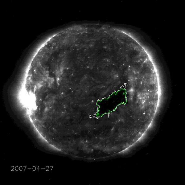
Figure 1. SOHO/EIT 195 Å image with an isolated non-polar coronal hole. The white contour indicates boundaries of the CH as selected by the described semi-automatic procedure. The green contour indicates boundaries of the CH defined by the automatic procedure.
Download figure:
Standard image High-resolution imageNext, we established an association between the variation of SW speed at 1 AU and individual CHs following the Abramenko et al. (2009) approach. SW speed measurements from the ACE spacecraft were searched for fast SW streams. Potential peaks were identified (using a 15 day average) and those exceeding one standard deviation level were highlighted for examination by the observer. In several cases, the observer included some clear peaks that were lower than the selected level due to a very high value or/and average value of standard deviation (caused by several high peaks during a 15 day average period). For the confirmed fast SW streams, the speed was calculated as an average of ACE measurements between the beginning and the end of a stream. Once the average time (t) and speed (v) at the ACE location were determined, the time (t0) when the stream left the solar surface was computed under the assumption that v is constant as

Figure 2 provides example of fast SW stream originating in the CH shown on Figure 1. In this plot, t0 is represented by the dotted vertical line and has a value of about 5.3 days (starting from 2007 April 22), t is about 8.13 days (vertical solid line), and the average speed within the stream, v (horizontal dashed line), is approximately 614 km s−1. The travel time derived from Equation (1) is 2.83 days.
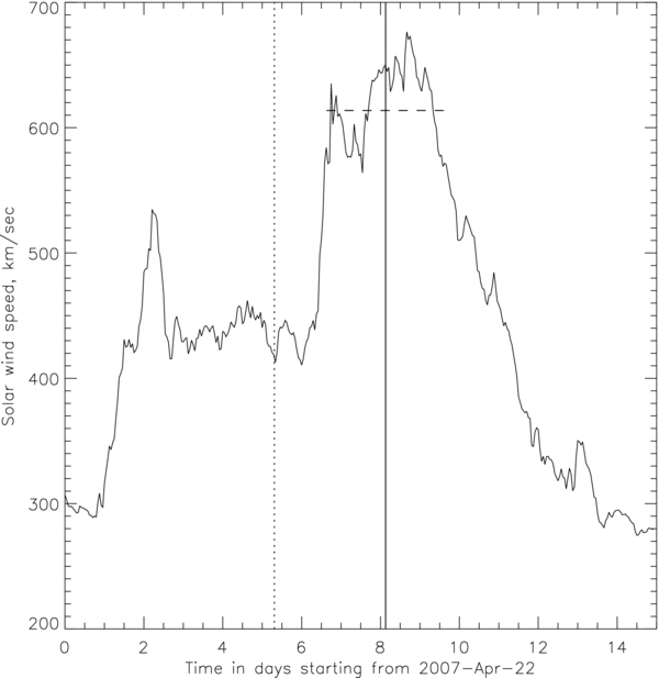
Figure 2. Temporal variation of the solar wind speed for the period from 2007 April 22 to 2007 May 7. The solid line shows the moment when the solar wind stream arrives to the Earth orbit and the dotted line shows the computed time when the stream should left the solar surface and the source must be near the central meridian. The dashed horizontal line indicates the average solar wind speed within the peak.
Download figure:
Standard image High-resolution imageAt the next step, images from SOHO/EIT for computed time (t0) were analyzed to identify a potential source of each stream. If EIT data showed the presence of an isolated CH (within approximately ±30 deg from the central meridian), the CH was selected for further study. We have only considered low-mid-latitude isolated CHs. Polar CHs and their low-latitude extensions were excluded.
The above procedure was applied to data from 1998 to 2008, and 108 CH fast SW stream pairs were selected for further investigation.
3. CORRELATION BETWEEN SOLAR WIND SPEED AND INTEGRATED PARAMETERS OF CHs
Several previous investigations studied correlations between the SW speed and different parameters of CHs. The best correlated parameters turned out to be the CH area (e.g., Nolte et al. 1976; Vršnak et al. 2007; Abramenko et al. 2009; Robbins et al. 2006) and integrated intensity or brightness of CHs (e.g., Luo et al. 2008; Obridko et al. 2009; Abramenko et al. 2009). These two parameters are often used in SW forecasting (e.g., Luo et al. 2008; Obridko et al. 2009; Vršnak et al. 2007; Robbins et al. 2006). However, these earlier studies were based on limited data sets. These included several CHs during certain years or those that had applied various restrictions on CHs and the exclusion of portion of CHs that fell outside of about 10 deg of the disk center (or considered brightness only in the darkest inner part of CHs; Nolte et al. 1976; Luo et al. 2008; Obridko et al. 2009; Vršnak et al. 2007). Also, it is unknown if the correlations between the area and intensity of CHs with SW are independent of each other. Our study removes some of these limitations.
As an additional justification, we note that the correlation between CBPs and fast SW speed has not been studied yet.
We have computed several different parameters for each CH to include the total area of CHs (without any restrictions) in the image plane, the deprojected area of CHs (in square degrees on solar surface), and the total intensity of all pixels inside CHs. In addition, we identified CBPs situated inside the CHs, and then calculated the area of CHs occupied by CBPs and their integrated brightness. For this study, a "coronal bright point" pixel was defined as any pixel situated inside the CH, the intensity of which exceeded the 1σ level above the mean intensity in the CH.
Table 1 lists Spearman's and Pearson's correlation coefficients between SW speed (VSW) and the area of CHs (ACH), the integrated intensity of CHs (ICH), the area of CHs occupied by CBPs (ACBPs), the integrated brightness of CBPs in CHs (ICBPs), the threshold used to define boundary of CHs (LCH), and the total brightness of the solar disk (IFD). Correlation coefficients for both the semi-automatic and automatic methods of identification of CH boundaries are shown.
Table 1. Correlation Coefficients Between the SW Speed and Other Calculated Parameters
| Parameters | Spearman's Rank | Significance of Its | Linear Pearson |
|---|---|---|---|
| Correlation Coefficient | Deviation from Zero | Correlation Coefficient | |
| VSW vs. ACH (deg) | 0.480 | 1.4 × 10⁻⁷ | 0.494 |
| VSW vs. ACH | 0.561 (0.553)a | 2.7 × 10⁻¹⁰ | 0.546 (0.492)a |
| VSW vs. ICH | 0.479 (0.465)a | 1.6 × 10⁻⁷ | 0.452 (0.343)a |
| VSW vs. ACBPs | 0.327 (0.422)a | 5.6 × 10⁻⁴ | 0.305 (0.295)a |
| VSW vs. ICBPs | 0.383 (0.408)a | 4.3 × 10⁻⁵ | 0.327 (0.246)a |
| VSW vs. f(ACH, ICH) | 0.471 (0.447)a | 2.7 × 10⁻⁷ | 0.445 (0.318)a |
| ACH (deg) vs. ICH | 0.837 | 1.7 × 10⁻²⁹ | 0.831 |
| ACH vs. ICH | 0.892 (0.945)a | 2.3 × 10-38 | 0.915 (0.921)a |
| ACH vs. LCH | −0.037 | 7.0 × 10⁻¹ | 0.026 |
| ACH vs. ACBPs | 0.649 (0.865)a | 3.1 × 10⁻¹⁴ | 0.744 (0.851)a |
| ACH vs. ICBPs | 0.775 (0.894)a | 8.1 × 10⁻²³ | 0.801 (0.838)a |
| ACH vs. IFD | −0.051 | 6.0 × 10⁻¹ | 0.031 |
| IFD vs. LCH | 0.855 | 5.5 × 10⁻³² | 0.880 |
| IFD vs. ICH | 0.304 | 1.4 × 10⁻³ | 0.331 |
| IFD vs. ICBPs | 0.335 | 3.9 × 10⁻⁴ | 0.360 |
| ICH vs. ICBPs | 0.888 | 1.7 × 10-37 | 0.923 |
| ICH vs. LCH | 0.356 | 1.5 × 10⁻⁴ | 0.374 |
Note. aValues in parentheses are for automatic mode for CH boundaries.
Download table as: ASCIITypeset image
Out of five parameters, the total area of CHs correlates most strongly with SW speed. The correlation is higher for the area measured in the image plane, ACH, as compared with the deprojected area, ACH (deg). We interpret this as an indication that the low-latitude parts of CHs have a larger contribution to the SW observed at the ecliptic plane as compared with high-latitude parts of CHs. This conclusion is in agreement with the early findings of Nolte et al. (1976).
Correlation between VSW and the integrated brightness of CHs is slightly weaker, but it is still statistically significant. To verify the uniqueness of each correlation, we investigated the possibility of multi-correlation: VSW = f(ACH, ICH), where f is a linear function of two parameters, in this case, the area of CH and the total intensity of CH. The correlation resulting from this multi-correlation analysis was found not to be stronger than the correlation between VSW and ACH or ICH. Therefore, we conclude that the correlation between the SW speed and the area of CH is the primary correlation, whereas the correlation between VSW and ICH is the result of an inter-correlation between the area and intensity of a CH. High correlation between ACH and ICH supports this conclusion (Table 1). Low correlation coefficients between parameters of CBPs and SW suggest that reconnection associated with CBPs does not play a significant role in SW acceleration.
Upon further investigation, we found that the correlation coefficient between the SW speed and CHs area changes depending on the level of solar activity. As a proxy for solar activity we used a total intensity integrated over the full solar disk. The results are shown in Table 2. It is clear that the correlation between VSW and ACH is lower during periods of high and low coronal brightness, which corresponds to maxima and minima of solar cycle, respectively. The correlation is significantly higher for the period of moderate activity—which is likely to correspond to the rising and declining phases of solar cycle. We see this change in the correlation to be in agreement with Robbins et al. (2006). However, our data for the moderate level of the coronal brightness (25 × 106 < IFD < 50 × 106 data number (DN)) include both rising and decaying phases of solar cycle, and therefore we cannot confirm if the correlation is higher for the declining phase, and if it is lower for the rising phase of the solar cycle as found by Robbins et al. (2006).
Table 2. Correlation Coefficients Between the SW Speed and Total Area of Associated CHs Depending on the Solar Activity Level
| Total Intensity over | Spearman's Rank | Significance of Its | Linear Pearson | Number of CHs |
|---|---|---|---|---|
| Full Solar Disk, 106 DN | Correlation Coefficient | Deviation from Zero | Correlation Coefficient | |
| I > 50 | 0.425 (0.390)a | 3.8 × 10⁻² | 0.408 (0.302)a | 24 |
| 50 > I > 25 | 0.657 (0.701)a | 4.9 × 10⁻⁹ | 0.645 (0.640)a | 63 |
| I < 25 | 0.395 (0.451)a | 7.7 × 10⁻² | 0.461 (0.538)a | 21 |
| All data | 0.561 (0.553)a | 2.7 × 10⁻¹⁰ | 0.546 (0.492)a | 108 |
Note. aValues in parentheses are for automatic mode for CH boundaries.
Download table as: ASCIITypeset image
The decrease in ACH–VSW correlation with solar activity could indicate additional contribution to SW from other sources (e.g., active regions, polar coronal holes), although to confirm that would require further study. Also, when the corona is too dim (at the minimum of the cycle), CH boundaries are difficult to determine (and are thus uncertain), which may affect the correlation between the area of CHs and SW speed during periods of low solar activity. The latter may be addressed by improved identification of CH boundaries using data observed at different spectral bands, such as (for example) recent data observed by the Solar Dynamics Observatory/Atmospheric Imaging Assembly.
Majority of the previous studies of the correlation between the SW speed and area (e.g., Luo et al. 2008; Obridko et al. 2009) used EIT 284 Å data. We used 195 Å data. As a control experiment, we have also applied our technique to EIT images taken in the 284 Å wavelength range. Although the correlation coefficients were slightly different, we did not find any change in our conclusions when using the 284 Å EIT data. We also find no statistically significant correlation between the area, brightness of CHs, and brightness level used to select the CH boundaries. As only a limited subset of the EIT 284 Å data was used for the above test, the resulting correlation coefficients are not included in Table 1.
4. SPATIAL DISTRIBUTION OF BRIGHT POINTS INSIDE CORONAL HOLES
To further investigate the role of CBPs in accelerating SW, we also studied the distribution of CBPs inside the isolated non-polar CHs that were observed in near-equatorial regions. Ten CHs during the period of 2002–2008 were chosen for that study. The following routine was applied to each selected CH.
- 1.Contours of a CH were defined as described in Section 2.
- 2.An intensity profile from each point at the boundary to the center of the CH (defined as a center of gravity using all pixels inside the CH) is constructed and recorded. All profiles are normalized by the "radius" of the CH, so that the distance changes from 0 (the center) to 1 (the boundary). An example of such a profile is shown in Figure 3. The Y-axis represents intensity along the profile and the X-axis is normalized distance (distance in pixels from the center divided by the radius, which is the distance from the center to the boundary). The radius is different for each profile, but after normalization all profiles would change along the X-axis from 0 to 1.
- 3.All distance-normalized profiles for each CH are averaged, and a Gaussian function is fitted to the average profile. This function represents a general trend in the intensity changes inside a CH from its center to the boundary. Subtracting this function from each individual profile allows us to better identify brightenings inside CHs and near its boundaries, as compared with the fixed intensity threshold.
- 4.All profiles are searched for bright pixels the intensity of which exceeds the average plus its standard deviation, and where the average is the mean of the difference between the individual profile and the best-fit function. All bright pixels satisfying these criteria are then recorded with their coordinates normalized by the profile radius.
- 5.A distribution of bright pixels inside the CH is computed and plotted using area normalized bins.
The computed average profiles of intensity inside CHs show the following patterns. A minimum brightness in a CH is about 0.6–0.86 of the brightness of the corona surrounding the CH, brightness reaches a minimum value at a distance of about 0.1–0.6 of the CH radius from the boundary of a CH, and the brightness profile inside the darkest portion of a CH is nearly flat. Figure 3 shows an example of a center-to-boundary profile for a selected CH (solid line) and a Gaussian function (dashed line) fitted to the average profile for this CH. A dash-dotted curve represents residuals after subtracting a fitted profile from the individual profile, and a solid horizontal line shows the threshold (≈6.7, DN) for the identification of bright point pixels inside this CH.
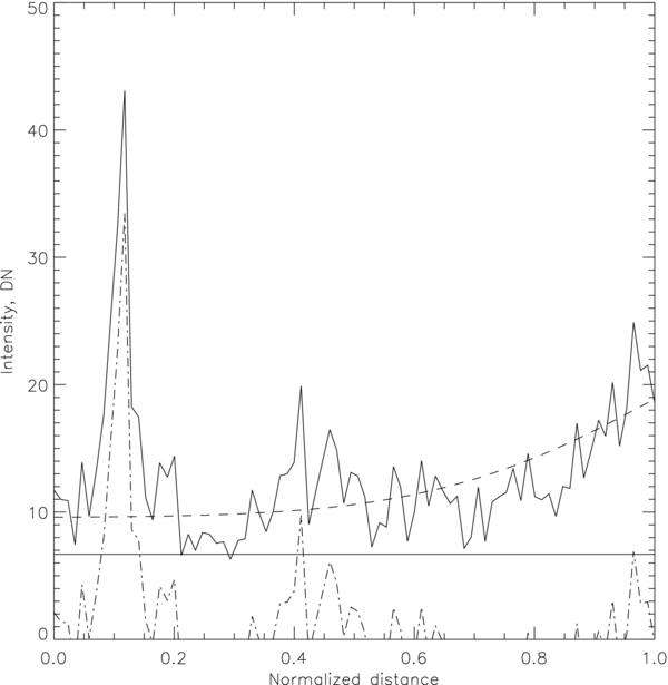
Figure 3. Individual profile of the intensity inside a CH (solid curve), best-fitted function (dashed curve), and their difference (dash-dotted curve). The straight solid line is a level for the bright pixel identification (average+standard deviation).
Download figure:
Standard image High-resolution imageFigure 4 gives us an example of a distribution of bright points pixels inside one of the CHs used in this study. The distribution is normalized, so all bins plotted along the X-axis (radius of the CH) have equal areas.
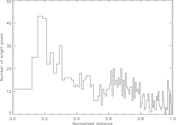
Figure 4. Distribution of "coronal bright points" pixels as a function of the normalized radius of the CH from the SOHO/EIT image for 2006 September 21. Bin sizes are normalized to represent equal areas.
Download figure:
Standard image High-resolution imageThe average distribution for all 10 control group CHs is presented in Figure 5. Note that the number of bright pixels here is also normalized and presented in percentages. From the plot one can see that the distribution shows a gradual increase in the number of bright pixels toward the center of the CH. According to the models, a CBP presents an example of the reconnection between two opposite polarities in a small magnetic bipolar structure observed on the photospheric level at the CBP location (Kankelborg & Longcope 1999; Golub et al. 1974; Webb et al. 1993; Longcope et al. 2001). Guided by this CBP–magnetic bipole association, we also calculated a distribution of small magnetic bipolar structures inside CHs. It was found that the number of small magnetic bipolar structures also increases toward the center of CHs, similar to the CBPs distribution.

Figure 5. Distribution of "coronal bright points" pixels as a function of radius of a CH for 10 control group CHs. Bin sizes are normalized to represent equal areas.
Download figure:
Standard image High-resolution image
5. DISCUSSION AND CONCLUSIONS
It is generally accepted that fast SW originates from the inner part of CHs. Our data show an increase in the number of CBPs and magnetic bipoles toward the center of CHs (Figures 4 and 5), which seem to support the idea that the fast SW can be driven by reconnection events (assuming that the CBPs are indicative of the reconnection).
On the other hand, from the interchange reconnection model one would expect to see more frequent reconnection events near the boundaries of CHs. Indeed, in four out of six cases, Subramanian et al. (2010) had reported there were more brightenings taking place at the boundaries of CHs. In two cases, they observed more brightenings inside CHs as compared with the boundaries. As Subramanian et al. (2010) have concluded, the reconnection events observed in their data sets can be responsible for driving slow SW. Although we do not see weak highly intermittent brightenings near the boundaries observed by Subramanian et al. (2010), we do see an increase in the number of (much brighter) CBPs in inner parts of CHs, suggesting that the reconnection may be a driver for both the slow and fast SW. However, we think that lack of a strong correlation between the CBP number and SW speed (see Table 1) may indicate that the reconnection associated with CBPs is not the primary mechanism for fast SW acceleration. This latter conclusion is in agreement with the Cranmer & van Ballegooijen (2010) arguments based on estimations of energy and timescales for Monte Carlo simulations, which deemed it unlikely that either the slow or fast SW is driven primarily by the reconnection and loop-opening processes at the scale of the "magnetic carpet" fields.
The strongest correlation with the SW speed is found with the total area of CHs. Unlike previous studies, we had considered the entire area of CHs, without any restrictions in latitude or central meridian distance. Still, a difference in the correlation between the total areas of CHs in the image plane and deprojected areas of CHs implies that equatorial parts of CHs provide the main contribution to faster SW as compared with high-latitude portions.
We have also established that SW–ACH is the primary correlation. Correlations between the SW speed and other parameters of CHs (including their brightness) are secondary and can be explained by the correlation of these parameters with the area of CHs (Table 1).
The correlation between the SW speed and area of CHs varies with the Sun's activity level. The highest correlation is observed during the periods of a moderate level of solar activity. The decrease in the correlation between VSW and ACH (for the periods of maxima and minima of solar activity) may indicate that other solar features contribute to the acceleration of the fast SW.
In summary, we conclude that it is unlikely that the reconnection events associated with CBPs can serve as the primary source of fast SW.
We are very grateful to V. Abramenko and V. Yurchyshyn for providing us with their software for the solar wind and coronal hole passage association. We also thank Ms. Jacqueline Diehl for her help in improving the text of manuscript. This work was supported by NASA NNH09AL04I inter-agency transfer. National Solar Observatory (NSO) is operated by the Association of Universities for Research in Astronomy, AURA, Inc., under cooperative agreement with the National Science Foundation. SOHO is a project of international cooperation between ESA and NASA. This research has made use of NASA's Astrophysics Data System Bibliographic Services.
Facilities: SOHO (EIT, MDI) - Solar Heliospheric Observatory satellite, ACE (SWEPAM) - Advanced Composition Explorer satellite