


ABSTRACT
We present the first analysis of the complete charge state distributions of heavy ions in interplanetary coronal mass ejections (CMEs), from singly charged to fully ionized. We develop a novel analysis technique that requires the combination and cross-calibration of two different data sets from the Solar Wind Ion Composition Spectrometer on the Advanced Composition Explorer. The first contains ions of higher charge states, and includes an identification of their mass, mass-per-charge, and energy-per-charge. The second data set contains singly and low-charge ions, and identifies only their mass-per-charge and energy-per-charge. Focusing on C, O, and Fe, we find ionic charge states representative of temperatures from ⩽60,000 K to over 5,000,000 K contained within interplanetary CMEs observed near 1 AU. We interpret these data in the context of near-Sun observations of filament material associated with CMEs. We find that singly charged ions are embedded within selected interplanetary CMEs, and we examine their densities and durations. These data thus provide the most unambiguous in situ diagnostic of solar prominence plasma in the heliosphere.
Export citation and abstract BibTeX RIS
1. INTRODUCTION
Coronal mass ejections (CMEs) expel plasma and magnetic flux from the solar surface into the heliosphere. Interplanetary coronal mass ejections (ICMEs) are the heliospheric remnants of these CMEs. While coronal observations show differences among CMEs, most are observed to have the same basic three-part structure: a bright rim, a low-density cavity, and a central core of cool, dense plasma. This core of cool plasma, generated via radiative cooling and typically found near magnetic neutral lines (Karpen & Antiochos 2008), is generally referred to interchangeably as a filament or prominence and is observed near the Sun in over 70% of CMEs (Gopalswamy et al. 2003). As filaments erupt into the heliosphere, they often trail the magnetically dominated cavities that result in so-called magnetic clouds (Klein & Burlaga 1982) or flux ropes. During the eruption process, these clouds dynamically interact with the ambient coronal and heliospheric plasmas, creating the bright rim due to the increased density in the interaction regions. Despite filaments being commonly observed at the Sun trailing the erupting clouds and interaction regions, relatively few observations of filament-related heavy ions have been made at 1 AU (Zwickl et al. 1982; Gopalswamy et al. 1998; Burlaga et al. 1998; Gloeckler et al. 1999; Lepri & Zurbuchen 2010).
Observed solar wind charge states typically correlate to coronal temperatures of 106 K or higher (von Steiger et al. 2000), but the cool temperatures in core filament plasma and incomplete ionization during CME eruption are expected to create lower ionic charge states. Using 12 years' worth of data from the Solar Wind Ion Composition Spectrometer (SWICS; Gloeckler et al. 1998) on the Advanced Composition Explorer (ACE; Stone et al. 1998), Lepri & Zurbuchen (2010) surveyed 283 ICMEs searching for plasma charge state signatures that would be expected in filament plasma. The very selective criteria in the study revealed significant enhancements in the density of extremely low charge state plasma (C2+, O2+, and Fe4+) in 4% of the ICMEs surveyed. Observed and modeled temperatures of filament core plasma indicate a local thermodynamic equilibrium temperature range of 15,000–40,000 K (Landi et al. 2010), and microwave observations show temperatures as low as 8000 K (Gopalswamy 1999), which are consistent with charge states as low as +1. With the exception of He1+ (Schwenn et al. 1980; Gosling et al. 1980; Skoug et al. 1999), these singly charged ionization states have been inaccessible by any previous analysis of ICMEs. Observations of these very low charge states would not only provide a test of the presence of these low-temperature plasmas, but would also provide a sensitive technique to constrain the effectiveness of ionization processes during the plasma's propagation throughout the heliosphere.
Lepri & Zurbuchen (2010) identified several ICMEs at 1 AU that had measureable density enhancements in low charge states of heavy ions, but the lowest charge states of those ions were not in the measurement range of the available data. We discuss in this paper the first observations of ICME plasma over the entire charge state range of C and O, and over the range Fe2+–Fe24+, which extend the previous observations using a novel analysis technique. Section 2 first provides details of the analysis technique used to derive these data. Section 3 then focuses on applying this new analysis to the identification of filament material, combining the data with a rich set of plasma and field measurements from ACE and providing a quantitative analysis of temperatures. Section 4 discusses the observed size and evolutionary characteristics of the filament plasma as it moves throughout the heliosphere. We conclude in Section 5.
2. ANALYSIS TECHNIQUES
Detections of filament material by ACE–SWICS were examined by Lepri & Zurbuchen (2010) in a comprehensive analysis based on heavy-ion composition. In that study, two-hour-averaged plasma composition data were analyzed with respect to unusually low charge states of C, O, and Fe. To identify these compositionally cold plasmas, specific criteria were used to avoid ions that are common in the solar wind, as well as avoid those whose densities were found biased for any reason, such as by the priority scheme used by the spacecraft telemetry. There were 11 events that fit these selection criteria, all of which were found to be associated with ICMEs. By comparing with CME observations from the Large Angle and Spectrometric Coronograph (Brueckner et al. 1995), 90% of these were linked to specific erupting filaments. This previous study utilized the improved and publicly accessible composition data of ACE-SWICS, which contain ionic charge states as low as C2+, O2+, and Fe4+, well below the typical dominant solar wind charge states of C5+, O6+, and Fe10+ that freeze-in near coronal electron temperatures of 1 MK. To search for singly and very low charged heavy ions in the ACE-SWICS data set, it is necessary to use different criteria for ion detection than those used by Lepri & Zurbuchen (2010).
Plasma data collected by SWICS covers an energy-per-charge (E/q) range of 0.49–100.0 keV e−1 and all masses from H to Fe. The SWICS instrument (Figure 1) is optimized for low-noise measurements of the elemental and charge state composition of solar wind plasma. A given solar wind ion is identified in the SWICS data by a combination of three independent measurements: an electrostatic selection of its energy-per-charge (E/q), a time-of-flight (TOF) measurement of its speed, and a measurement of its total energy. A series of voltage settings are sequentially scanned in the electrostatic analyzer to select ions within a chosen E/q passband. Prior to a measurement of its energy and speed, an ion is accelerated within the instrument in proportion to its ionic charge by an electrostatic potential. This acceleration of 21–26 kV significantly reduces the amount of energy straggling and angular scattering that the ion experiences when it traverses the instrument's thin carbon foil. The carbon foil emits secondary electrons to trigger a start signal (1) for a TOF measurement. The acceleration allows most ions to overcome the energy threshold of the solid-state detector (SSD), where the residual energy (3) is measured. When the ion impacts the SSD, secondary electrons are emitted and are used to trigger a stop signal (2) for the ion TOF. The speed of the ion is calculated from the start and stop signals of the ion TOF across a known distance. The three detectors, marked 1–3 in Figure 1, provide the necessary signals for a triple-coincidence measurement.

Figure 1. Illustration of the SWICS electrostatic analyzer and TOF system. Numbered detectors indicate the start (1), stop (2), and energy (3) measurements of a triple-coincidence event. Figure adapted from Gloeckler et al. (1998).
Download figure:
Standard image High-resolution imageLinking the E/q of an ion to the measurement of its energy and speed allows the mass and charge of the ion to be calculated unambiguously, within the limits of the resolution of the SWICS instrument. The start, stop, and energy requirement of triple coincidence for each ion creates the highest standard of measurement. All SWICS solar wind data processing of triple-coincidence data follows the methodology given in the Appendix of von Steiger et al. (2000).
As heavy ions with low charge states pass through the acceleration region, they typically do not gain acceleration sufficient to overcome the energy detection threshold of the SSD, around 25–35 keV for H and He, and >50 keV for heavier elements (Ipavich et al. 1978; von Steiger et al. 2000), and are therefore absent or underrepresented in the triple-coincidence data. Although they may not be detected by the SSD, these ions may still trigger the start and stop detectors for the TOF measurement, creating a double-coincidence event. The TOF measured in a double-coincidence event can be combined with the E/q to calculate the mass-per-charge (M/q) of the ion. Without a direct measurement of the energy, however, ions with similar M/q values cannot easily be distinguished from each other even if they have different energies (e.g., He1+, C3+, and O4+ each have 4 amu e−1). This loss in resolution makes ion identification in the double-coincidence measurement ambiguous for most ions. Fortunately, singly charged heavy ions are often isolated from other ions in M/q and can be readily identified.
Singly and doubly charged ions can originate in the heliosphere, where interplanetary dust and neutral gases experience ionization and are picked up by the solar wind (Grün & Landgraf 2001; Gloeckler et al. 2000). Similarly, neutral gas from interstellar space can drift into the heliosphere, become ionized, and be picked up by the solar wind (Gloeckler et al. 1993). Both of these populations of singly charged particles are observed to have velocity distributions unique to pickup ions, and are therefore generally much hotter that the solar wind, with a sonic Mach number near 1. In contrast, typical Mach numbers for solar wind heavy ions in the ACE-SWICS data are 5–20 at 1 AU, making it possible for singly charged pickup ions to be distinguished from singly charged ions of solar origin. Previous studies that have examined heavy elements in low charge states, such as SWICS analyses of singly charged interstellar and inner-source pickup ions (e.g., Gloeckler & Geiss 1998), have focused exclusively on double-coincidence measurements. Singly and doubly charged cold filament plasma, if present in ICMEs, would also be found in the SWICS data using an analogous double-coincidence measurement methodology. Depending on their ionic charge states, some heavy ions can be observed in both double and triple coincidence, so a combination of the two data sets is necessary to obtain the full picture.
Measurements taken during an ICME on 2005 January 9 are shown in Figure 2. The data are accumulated during only the filament portion of the ICME, as explained in detail in Section 3. In Figure 2(a), the mass of each ion is plotted against the M/q for triple-coincidence measurements, with the color scale indicating the number of counts. The locations of many heavy-ion charge states of He, C, O, and Fe are outlined by black ovals. The double-coincidence data (Figure 2(b)) are plotted in terms of the E/q against the M/q, with counts shown by the color scale. A close examination of the double-coincidence data also shows significant amounts of heavy ions with high charge states—ions that should have overcome the energy threshold of the SSD and triggered a full triple-coincidence measurement. The detection efficiency of the SSD improves with increasing energy for a given ion species, but is not near 100% for heavy ions at solar wind energies. Ions that are prominent in the solar wind, such as Fe8+–Fe10+ or O6+, will have a high enough flux that the fraction overlooked by the SSD will play a significant role in the double-coincidence data, particularly in M/q ranges where these ions overlap low-charge-state heavy ions. To ensure that densities and velocity distributions in the triple-coincidence data are minimally affected by the "missing" ions that go into the double-coincidence measurement, detector efficiencies are accounted for during data processing (von Steiger et al. 2000). For this study, where the double- and triple-coincidence data sets are combined, corrections for the detector efficiencies are applied only to the double-coincidence data.
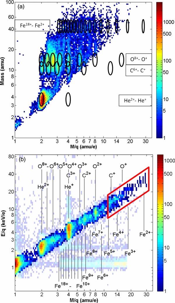
Figure 2. Ion charge state composition data for the filament material in a 2005 January 9 ICME. The triple-coincidence data (a) capture the higher charge states of heavy ions, including carbon, oxygen, and iron. The labeled ion charge states are marked by black ovals. The double-coincidence data (b) contain ions that do not trigger a signal on the SSD and include singly charged heavy ions. The M/q region that was used for the combined data set in this study is outlined in red.
Download figure:
Standard image High-resolution imageAn ion event was only counted if the ion speed was within 15% of the average hourly He2+ speed. The noise reduction from this criterion is illustrated well in the double-coincidence data of Figure 2(b), where the events that satisfy the speed requirement are visible as a bright-colored diagonal strip. Vertical data streaks near M/q values of 1 (H+) and 4 (He1+) are also visible, with a smaller streak near M/q = 2 (He2+). These are the indications of the suprathermal contributions to the solar wind distribution functions of H+ and He2+, as well as the hot pickup ion distribution of He1+ (Möbius et al. 2004). The horizontal streaks in Figure 2(b) at around 1 keV e−1 and 2 keV e−1 are likely due to a combination of energy straggling of solar wind H+ and He2+ in the carbon foil, slowing some of the ions down so much that their recorded TOF aligns with a range of high M/q values; and so-called accidental coincidence measurements, where two separate ions trigger the start and stop signals for a TOF, leading to an M/q value that is unassociated with the original ions. These horizontal streaks are mostly associated with the E/q ranges of protons and He2+, which are the most abundant ions in the solar wind. Singly charged ions can be identified in the double-coincidence data, but due to the overlap in ions with similar M/q, such as C2+ and Fe9+, it is difficult to unambiguously identify ions below ∼10 amu e−1. The double-coincidence data range used for this study (M/q > 11 amu e−1) is outlined in red. The two data sets complement each other, providing a full charge spectrum for several atoms.
Once an event has been detected by SWICS, it must be classified correctly in terms of its ion species. For triple-coincidence data, the identity of the measured ion is statistically determined by processing the E/q, TOF, and measured energy in a parameterized forward model, which is constrained by results from laboratory calibrations (Gloeckler et al. 1998; von Steiger et al. 2000). For the double-coincidence data, the measured E/q and TOF of each event are used in the calculation of the M/q, as shown in Equation (1). Other necessary parameters include the travel times of the TOF start and stop electrons (Tstart, Tstop), which can be determined from an ion optics model of the SWICS TOF telescope using SIMION software (Dahl 2000); the length of the TOF telescope from carbon foil to SSD (L); the acceleration voltage that the ion experiences prior to entering the TOF telescope (VA); and the energy loss (see the Appendix) experienced in the carbon foil (Eloss), calculated with Monte Carlo techniques in the program The Stopping and Range of Ions in Matter (SRIM; Ziegler et al. 2010):
For the full, combined data set used in this study, the double- and triple-coincidence measurements were binned into matching 1 hr time steps from their native 12 minute resolution. Densities were calculated using the method described in von Steiger et al. (2000), and the data were filtered by speed and M/q as described previously. Corrections were applied to the double-coincidence data to account for detector efficiencies in the start and stop microchannel plate detectors. The densities of double- and triple-coincidence data were then added together to create the combined data set used for this study. As can be seen in Figure 2(a), the ions C1+, O1+, and Fe2+, marked by empty ovals, do not register any counts on the SSD; and Fe+, with an M/q of 56 amu e−1, is outside of the measurement range. The double-coincidence data outlined in Figure 2(b) fill in a region of M/q space that is missed by the triple-coincidence measurements, thereby extending the SWICS data set to its lowest measured charge states.
3. SINGLY CHARGED FILAMENT PLASMA
Each of the ICME time periods identified by Lepri & Zurbuchen (2010) was examined for low charge states in the ACE–SWICS double-coincidence data. Figure 3 shows an event from 2005, with ICME boundaries marked with black vertical lines, the duration of cold plasma indicated by a colored stripe, and the boundaries of a previous ICME marked with blue vertical lines. ICME boundaries are inferred using both solar wind plasma and magnetic field data as described in Cane & Richardson (2003) and Richardson & Cane (2010), and periodically updated boundary information is available online at the ACE Science Center: http://www.srl.caltech.edu/ACE/ASC/DATA/level3/icmetable2.htm. The panels of the figure show data taken by sensors onboard the ACE spacecraft: the proton speed, density, and temperature measured by SWICS and the Solar Wind Electron Proton Alpha Monitor (SWEPAM; McComas et al. 1998); the hourly charge state distributions of iron, oxygen, and carbon from SWICS, with hourly averages marked by a solid black line; and the magnetic field magnitude from the magnetic field experiment (MAG; Smith et al. 1998). The double-coincidence measurements add to the data set the +1 charge states of carbon and oxygen, and the +2 charge state of iron, as well as augmenting the triple-coincidence +3 and +4 iron charge states. These inclusions provide a more complete picture of the ion charge state distributions and indicate that the filament material was indeed frozen-in at the lowest charge states of at least C and O.

Figure 3. Cold filament plasma in a 2005 January 9 ICME. Charge states as low as C1+, O1+, and Fe2+ are observed during the filament, which is contained within the shaded vertical stripe. The ICME boundaries are shown in black solid (beginning) and dashed (end) vertical lines. A prior ICME is marked with blue vertical lines.
Download figure:
Standard image High-resolution imageThe duration of the interval of low charge plasma within the ICME was longer when the full data set was considered than when using just the triple-coincidence data. Density enhancements in C1+ can be found 2 hr earlier than the other charge states of carbon. A concentration of Fe2+ is found coincident with the time of the peak C1+ and O1+ densities, on day 9 from 09:00 to 11:00. A density enhancement of cool, low charge state plasma on DOY 8 is also observed, when another ICME passed by the ACE spacecraft; this time period does not show an enhancement in cold charge states in the triple-coincidence data. Although the TOF of Fe1+ lies outside of the timing window cutoff of SWICS, measurements of filament temperatures (Gopalswamy et al. 1997) and calculations of charge state fractions at various temperatures (Landi et al. 2012) indicate that, were the SWICS cutoff limits adjusted to measure it, Fe1+ would possibly be found in some of the SWICS ICME data as well.
Figure 4 shows average hourly densities for each measured charge state of C, O, and Fe during the shaded interval of the filament material embedded within the 2005 January 9 ICME. Double- and triple-coincidence measurements have been combined into a full data set as explained previously. Densities from charge states found only in the double-coincidence data are shown in red, triple-coincidence in blue, and charge states found in both double- and triple-coincidence data are shown in purple. For reference, the typical solar wind proton density at 1 AU is in the range of 2–10 cm−3. The density of carbon (Figure 4(a)) is highest for the charge state C2+ and decreases for higher charge states until rising again for C6+. When the measured densities of oxygen in the filament are examined by their charge state (Figure 4(b)), a clear double peak is seen, with enhancements in O2+ and in the nominal solar wind values of O6+. For iron (Figure 4(c)), there are density peaks at three charge states. The cold filament material has a peak around Fe3+–Fe5+, while the other two peaks match the iron bi-modal charge state distribution, which is found in 95% of all ICMEs, around charge states Fe8+ and Fe16+. While ICMEs have been observed to contain plasmas of different temperatures moving together (e.g., Landi et al. 2010), it is also possible to obtain this bi-modal charge state signature as a result of fast heating of dense plasma followed by a rapid cooling due to expansion (Gruesbeck et al. 2011).

Figure 4. Hourly average densities of C, O, and Fe charge states from the filament material of the 2005 January 9 ICME. Double-coincidence data are shown in red, triple-coincidence data are shown in blue, and charge states containing densities from both data sets are shown in purple. Charge states as low as C1+, O1+, and Fe2+ can be measured in this full data set.
Download figure:
Standard image High-resolution imageThe presence of very low charge states indicates that at least part of the ICME plasma is very cold, <100,000 K. For reference, Figures 5(a)–(c) show the fraction of C, O, and Fe ions distributed in each charge state as a function of temperature. These fractions have been calculated using the CHIANTI ionization and recombination data (Dere et al. 1997; Landi et al. 2012) under equilibrium conditions, so they are not likely representative of ICME plasma. Realistic charge state distributions can be calculated only by considering the evolution of the plasma density and temperature as the ejecta travel far from the Sun. Still, they clearly indicate that at typical prominence temperatures (10,000–100,000 K) the low charge states dominate, and will be the starting ionization distribution from which the ICME plasma will evolve. For reference, the vertical shaded regions indicate the temperature range that could create the charge state distributions seen in the 2005 January 9 ICME.

Figure 5. Fractional abundances of C, O, and Fe, calculated from CHIANTI recombination and ionization data. The abundances are shown as a function of coronal electron temperature in conditions of thermodynamic equilibrium. The shaded regions indicate the temperature range that could create the charge state distributions seen in the 2005 January 9 ICME.
Download figure:
Standard image High-resolution imageA visual comparison of Figures 4 and 5 indicates that under equilibrium conditions, coronal electron temperatures of <100,000 K will create low charge state ions in the abundances observed in the ICME filament material. This is consistent with remote observations of CME core plasma temperatures near the Sun (Landi et al. 2010).
4. ANALYSIS AND DISCUSSION
Out of the 11 ICME events defined in the Lepri & Zurbuchen (2010) list, 8 of them occurred in time periods where double-coincidence measurements were available in the ACE–SWICS data set. The cold events observed during ICMEs are listed in Table 1, along with the duration of the low charge state plasma for both the full data set and the triple-coincidence only. The average solar wind speed is from SWICS proton measurements. The observed filament dimension is derived from the combined data set and the average solar wind speed during the filament observations. For the cold ICME events examined here, the average duration is 14.6 hr, about 20% longer than what was observed using triple-coincidence only. The average derived dimension is around 0.1–0.2 AU, which is indicative of the large spatial expansion that filament plasma undergoes as it moves from the Sun into the heliosphere. Each of these ICMEs exhibited density enhancements in one or more of the lowest measurable heavy-ion charge states. The extended SWICS data set not only reveals colder ICME freeze-in temperatures for the filament plasma, but also generally longer durations.
Table 1. Characteristics of Cold ICME Material
| Year | DOY, UT | Duration (hr) | Duration (hr) | Solar Wind Speed | Filament Dimension |
|---|---|---|---|---|---|
| Combined Data Set | Triple-coincidence Only | (km s−1) | (AU) | ||
| 1998 | 122 08:10–123 00:11 | 16.0 | 16.0 | 579 | 0.22 |
| 1999 | 107 00:58–107 17:27 | 16.5 | 8.2 | 400 | 0.16 |
| 1999 | 227 05:54–227 20:01 | 14.1 | 9.1 | 374 | 0.13 |
| 2000 | 52 02:59–52 22:13 | 19.2 | 16.0 | 427 | 0.20 |
| 2001 | 295 08:00–295 15:00 | 7.0 | 7.0 | 542 | 0.09 |
| 2002 | 252 22:03–253 14:54 | 16.8 | 12.8 | 407 | 0.16 |
| 2003 | 300 20:15–301 09:01 | 12.8 | 12.8 | 550 | 0.17 |
| 2005 | 9 06:00–9 20:01 | 14.0 | 12.0 | 446 | 0.15 |
Download table as: ASCIITypeset image
Each of these ICMEs contains cold filament material with singly charged heavy ions, but not all low-charge ions were enhanced equally during the filament. In general, the C1+ showed the clearest enhancements, and often was enhanced for the longest duration, while the density enhancements of Fe2+ would sometimes only be observed in one of the hourly accumulations. In each of these cold ICMEs, the densities of ions with elevated charge states were also enhanced, as shown in Figure 6. During this ICME from 2002 September 9 to 10, enhancements were seen simultaneously in densities of iron charge states near both Fe8+ and Fe16+. During the time period of detected filament material (shaded region), however, those density enhancements in the hot charge states fade and densities increase in the lower, cold charge states. After the main concentration of cold plasma passes, the densities of hot charge states increase again. The timing of the hot and cold plasma is in general agreement with the shape of a passing flux rope (Lin et al. 2004). Observations of plasma in the leading edge of the flux rope show a hot, dense population. This is followed by a measurement of cool low-density plasma as the spacecraft passes through the core. Finally, the trailing edge has similar hot charge states as the leading edge. The times when densities are enhanced in both hot and cold charge states simultaneously confirm the findings of plasma mixing reported in previous ICME studies (e.g., Zwickl et al. 1982; Gloeckler et al. 1999; Lepri & Zurbuchen 2010), and support the observations of Landi et al. (2010), in which the CME core consists of two components: a cold, dense concentration of plasma traveling together with a hot, low-density component. For the ICMEs studied here, the cold plasma was observed to be near the leading edge, trailing edge, or in the middle of the ICME with almost equal probability.
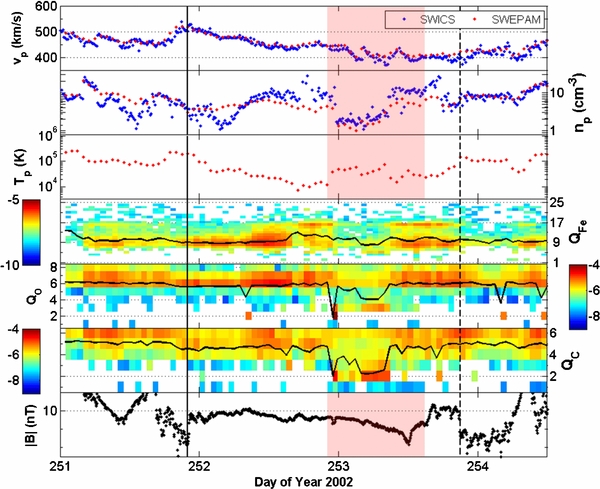
Figure 6. ICME in 2002 with clear bi-modal and cold charge states. In the iron charge state distribution around day 253, density enhancements can be seen around the +8 and +16 charge states. During part of the detection of the cold material (shaded region), the density enhancements of high charge states disappear and lower charge states of iron (+4, +5) are enhanced.
Download figure:
Standard image High-resolution image5. CONCLUSIONS
We present the first full charge state distributions of heavy ions embedded within ICMEs. These measurements include plasma charge states as low as singly charged carbon and oxygen, and the +2 charge state of iron, which is the lowest measurable charge state of iron attainable by SWICS. The charge state distributions of C and O correspond to what would be created in equilibrium conditions near the Sun at around 80,000–100,000 K or lower. The SWICS instrument is not designed to observe neutral particles, so the possibility cannot be ruled out that at very cold temperatures a population of neutral material may exist. These observations of cold material were made applying a novel technique that combines a data set of ACE–SWICS double- and triple-coincidence data to eight selected ICMEs from the Lepri & Zurbuchen (2010) cold plasma survey.
The average duration of the cold material within ICMEs is longer in the full data set than what was seen using triple-coincidence data alone. On the average, when low and singly charged ions are included, the duration of filament-associated plasma is increased by 20%; individual ICMEs show increases in duration of up to a factor of two. The geometric dimension of plasma with compositional signatures from filaments is derived from our observations to be 0.1–0.2 AU. Furthermore, the location of cold filament material does not appear biased to any location within the ICME, consistent with the findings of the Lepri & Zurbuchen (2010) study.
The estimated freeze-in temperatures for the charge state distributions of cold material observed by ACE–SWICS correspond to remote observations and models of filament temperatures in the low corona, adding support to the association of these cold events with filamentary eruptions. While the majority of CMEs are observed to be associated with filament material near the Sun, the observations of concentrations of cold filament material at 1 AU are rare. There are physical processes that must be understood to fully explain how this cold material is preserved as it propagates from its low freeze-in altitude through the hot, multimillion degree corona and out to 1 AU. These observations provide additional constraints on models of CME initiation and expansion within the corona and into the heliosphere.
The authors acknowledge J. Thomas and J. M. Raines for assistance with the access and processing of ACE-SWICS data. This work was supported in part by NASA grants NNX10AQ61G, NNX08AI11G, NNX11AC20G, and NNX10AM17G.
APPENDIX: CARBON FOIL ENERGY LOSS MODEL
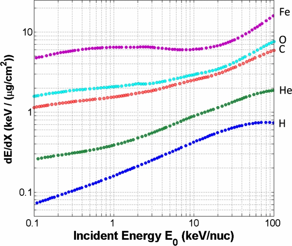
To calculate the M/q of an ion from the TOF measurement, the energy loss it experiences when passing through the thin carbon foil must first be identified. This energy loss is highly dependent on the mass and charge state of the ion, and has been characterized experimentally for ions of several energies (Ipavich et al. 1982; Allegrini et al. 2006). This energy loss can also be found using the program SRIM (Ziegler et al. 2010) and the general procedure outlined here. The advantages of the SRIM-based model include the flexibility of choice with respect to energy range, foil thickness, and ion species, as well as the database of thousands of experimental measurements upon which the SRIM calculations have been corrected and calibrated (Ziegler 2004). Thin carbon foils have been found to have layers of surface impurities that thicken the foil (Funsten et al. 1993) and may affect the ion-stopping properties. An approximation will be made here of a pure carbon foil of arbitrary thickness, with a density of 2.253 g cm−3. Ion stopping and range tables can be tabulated in SRIM for each element over a specified energy range. The calculation gives both the electronic and nuclear stopping powers, which must be summed together to find the total stopping power (dE/dX). In Figure 7, the stopping power is shown for several elements passing through carbon as a function of the incident energy-per-nucleon (E0), which is what the ion possesses at the time of foil impact, and therefore includes any energy gained in the acceleration region.
Figure 7. SRIM calculations of energy loss, dE, experienced by an ion passing through a carbon foil of thickness dX, as a function of incident energy-per-nucleon for H, He, C, O, and Fe. The solar wind typically has about 1 keV nucleon−1.
Download figure:
Standard image High-resolution image
A generally applicable model of energy loss through thin carbon foils would account for the full energy measurement range of all charge states of H–Fe in multiple space plasma instruments, e.g., MESSENGER-FIPS (0.46–20 keV e−1; Andrews et al. 2007), SWICS (0.49–100 keV e−1), and Wind-STICS (30–230 keV e−1; Gloeckler et al. 1995). The stopping power of carbon can be tabulated for each incident element over the energy range of the instrument and plotted against E0 as shown in Figure 7. By fitting equations to these curves, the stopping power dE/dX can quickly be found for any E0, and can be multiplied by the thickness of the instrument's carbon foil (dX, in units of μg cm−2) to find the energy lost (dE) by a traversing ion.