


ABSTRACT
Focused particle transport in a nonuniform large-scale magnetic field is investigated numerically in the case of isotropic pitch-angle scattering. Evolving particle density profiles and distribution moments are computed from solutions of a system of stochastic differential equations, equivalent to the original Fokker–Planck equation for the particle distribution. Conflicting analytical predictions for the transport coefficients in the diffusion limit, independently calculated by Beeck & Wibberenz and Shalchi, are compared with the numerical results. The reasons for the discrepancies among the analytical and numerical treatments, as well as the general limitations of the diffusion model, are discussed. The telegraph equation, derived in a higher-order expansion of the particle distribution function, is shown to describe the particle transport much more accurately than the diffusion model, especially ahead of a moving density pulse.
Export citation and abstract BibTeX RIS
1. INTRODUCTION
Cosmic-ray transport in turbulent cosmic magnetic fields is often investigated using the Fokker–Planck equation (e.g., Schlickeiser 2011 and references therein). When the particle pitch-angle distribution is nearly isotropic, a perturbed Fokker–Planck equation can be integrated over the pitch angle, yielding a simpler diffusion equation for the particle density (Jokipii 1966; Hasselmann & Wibberenz 1968). The diffusion approximation should be valid as long as the scale of density variation is significantly larger than the particle mean free path. Hasselmann & Wibberenz (1970) derived a theoretical expression for the coefficient of spatial diffusion κ|| parallel to a constant mean magnetic field. The value of κ|| was shown to be determined by an appropriate average of the pitch-angle scattering coefficient in the Fokker–Planck equation. Numerical studies confirmed the accuracy of the theoretical predictions based on the diffusion approximation (Kóta et al. 1982).
The original formulation of the diffusion approximation neglected the adiabatic focusing effect due to a spatially varying mean magnetic field. Large-scale magnetic fields, however, are often nonuniform in space plasmas. Unless the particle mean free path is negligibly small compared with the magnetic field length scale, adiabatic focusing should strongly modify the particle transport parallel to the field (Roelof 1969; Earl 1976; Kunstmann 1979).
Focused transport equations have been used extensively to model the propagation of energetic particles in interplanetary space following large solar flares (e.g., Bieber et al. 2002; Sáiz et al. 2008; Dröge et al. 2010). Notably, Artmann et al. (2011) employed a focused diffusion model to interpret the flare electron spectra obtained with the Wind spacecraft. Tautz et al. (2012) list several other applications of focused particle transport in astrophysics.
Beeck & Wibberenz (1986) derived the diffusion approximation taking into account adiabatic focusing (see also Earl 1981). Adiabatic focusing both modifies the parallel diffusion coefficient κ|| and causes coherent streaming of cosmic-ray particles, quantified by the coherent speed u. Litvinenko (2012a, 2012b) revisited and generalized the diffusive limit of focused particle transport by analyzing a system of stochastic differential equations equivalent to the Fokker–Planck equation. Litvinenko (2012b) concluded that, in the limit of vanishing magnetic helicity, the resulting expressions for κ|| and u were those in Beeck & Wibberenz (1986). Independently, Shalchi (2011) proposed a new method for calculating κ||, based on the Kubo (1957) formalism. Shalchi (2011) obtained a formula for κ||, which disagreed with the expression in Beeck & Wibberenz (1986) except in the limit of a constant mean magnetic field.
Concrete values of transport coefficients are of obvious importance in applications. To evaluate the validity of the conflicting theoretical results, we present in this paper numerical solutions of the Fokker–Planck equation. We compute the dependence of the solutions on the strength of adiabatic focusing, measured by a focusing length L, and we compare the numerical results with the theoretical predictions of the diffusion approximation. In order to emphasize the essential points of the analysis, throughout the paper we consider the Fokker–Planck equation with isotropic pitch-angle scattering, in which case the theoretical formulas for the transport coefficients are particularly simple. It would be straightforward to incorporate the effects of non-isotropic scattering, using, e.g., the transport equations in Litvinenko (2012b). Our goal, however, is to emphasize the general limitations of the diffusion model, and so we choose to work with the simplest physically meaningful model.
2. ANALYTICAL ARGUMENTS
2.1. Theoretical Description of Focused Transport
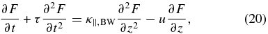
The Fokker–Planck equation for a cosmic-ray distribution function, which incorporates the effects of pitch-angle scattering and adiabatic focusing, is given by
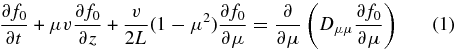
(e.g., Roelof 1969; Earl 1981). Here f0 is the distribution function of energetic particles (gyrotropic phase-space density), t is time, μ is the cosine of the particle pitch angle, v is the particle speed, z is the distance along the mean magnetic field B0, L = −B0/(∂B0/∂z) is the adiabatic focusing length, and Dμμ is the Fokker–Planck coefficient for pitch-angle scattering. For simplicity, momentum diffusion is neglected. In practice, momentum diffusion can be neglected for the transport of solar energetic particles in interplanetary space (Artmann et al. 2011).
As a concrete illustration, throughout this paper we assume a constant focusing length, L = const, and isotropic pitch-angle scattering:

where D0 = const. An exact steady solution of Equation (1) is then given by
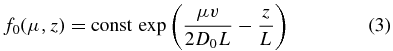
(Kunstmann 1979; Roelof 1969). Physical regimes leading to isotropic pitch-angle scattering have been analyzed by Shalchi et al. (2009).
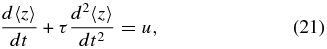
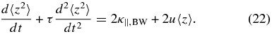
Numerical studies of particle transport often employ the fact that a system of stochastic differential equations contains the same information about the evolution of the particle distribution as the Fokker–Planck equation (e.g., Fichtner et al. 1996; Zhang 1999; Pei et al. 2010; Dröge et al. 2010; Strauss et al. 2011). In particular, standard application of the Itô calculus (e.g., Litvinenko 2012a) shows that Equation (1) in the case of isotropic pitch-angle scattering and L = const is completely equivalent to the system


where W(t) represents a Wiener process with zero mean and variance t (Gardiner 2009).
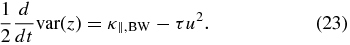
2.2. The Diffusion Approximation
If the time-dependent angular distribution of energetic particles remains close to that of the exact Equation (3), integration of a perturbed Fokker–Planck equation over μ leads to the diffusion approximation for the evolution of the particle density. As shown by Beeck & Wibberenz (1986), the resulting equation for the isotropic linear density
is as follows:
In Equation (7),
is the coherent speed, and κ|| is the parallel diffusion coefficient. Because this mode of particle transport comprises both coherent streaming and diffusion, Earl (1981) called it pseudo-diffusion.
Note for clarity that the sign of the convective term in Equation (7) is different from that in Equation (17) in Beeck & Wibberenz (1986). This is because Beeck & Wibberenz (1986) used the phase-space density, whereas Equation (7) is written for the linear density, defined as the number of particles per line of force per unit distance parallel to B0. The two descriptions are mathematically equivalent (Earl 1981). Because the mean magnetic field is proportional to exp (− z/L), the cross-sectional area of a flux tube scales as exp (z/L), and so the particle conservation is conveniently expressed as N(t) = 2∫Fdz = const.
Clearly κ|| is the key parameter controlling the particle transport. Beeck & Wibberenz (1986) derived an expression for κ|| in terms of the pitch-angle scattering rate Dμμ and the focusing length L. In the limit L → ∞, the expression for κ|| reduces to that in Hasselmann & Wibberenz (1970). When scattering is isotropic, Equation (14) in Beeck & Wibberenz (1986) yields
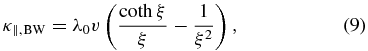
where ξ = λ0/L is the focusing parameter, and

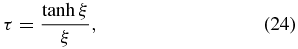
is the scattering mean free path in the absence of focusing (e.g., Equation (3) in Beeck & Wibberenz (1986)). By contrast, a recent calculation by Shalchi (2011) leads to a different expression for κ|| = λv/3. Equation (33) for the scattering length λ in Shalchi (2011) yields
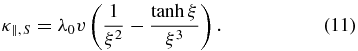
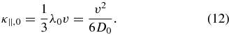
Clearly the two expressions for the parallel diffusion coefficient are contradictory, except in the limit of no focusing, ξ → 0, when both expressions yield
Shalchi (2011) did not discuss the earlier calculations by Earl (1981) and Beeck & Wibberenz (1986).
Since the diffusion approximation is the standard approximation for studying the cosmic-ray transport (e.g., Kóta et al. 1982; Schlickeiser & Shalchi 2008; Artmann et al. 2011), the discrepancy between κ||, BW and κ||, S is troubling. To evaluate the validity of the conflicting theoretical results, below we present numerical solutions of the Fokker–Planck equation. We compute an evolving spatial density profile F(z, t) and compare the numerical results with the theoretical predictions of the diffusion approximation. We also investigate the predicted and computed dependencies of the solutions on the focusing parameter ξ.
The validity of the diffusion approximation usually requires that the focusing be sufficiently weak, say ξ < 1. Both expressions for the parallel diffusion coefficient, however, are formally valid for an arbitrary ξ. In the next section, we determine the dependence of our numerical results on the focusing strength in a sufficiently wide range 0 ⩽ ξ ⩽ 2, which simplifies the comparison of the numerical and analytical results.
3. NUMERICAL RESULTS
3.1. Stochastic Simulations
We solved the Fokker–Planck Equation (1) for a range of focusing strengths and time intervals by integrating the stochastic differential Equations (4) and (5). We introduced dimensionless variables by measuring distances in units of the mean free path λ0 = v/2D0, speeds in units of the constant particle speed v, and times in units of λ0/v = 1/2D0. The dimensionless stochastic equations are as follows:

where we used the identity W(a2t) = aW(t). The only parameter of the simulation is the dimensionless focusing strength ξ that we vary in the range 0 ⩽ ξ ⩽ 2. The parallel diffusion coefficients are normalized by λ0v = v2/2D0, which gives the dimensionless κ||, 0 = 1/3 in a uniform mean magnetic field (ξ = 0).
The stochastic equations are more convenient to work with than the original Fokker–Planck equation. We solve Equations (13) and (14) using the Milstein approximation scheme:

where  t is a normal random variable with mean zero and variance unity (Kloeden & Platen 1999). Particles are reflected at μ = ±1 to conserve probability at these boundaries. Most conveniently, particle distribution moments are obtained simply by evaluating the appropriate sample moments from the particle simulations.
3.2. Evolving Particle Distributions
The numerical results described in this section correspond to a delta-functional initial distribution in position and isotropic pitch-angle distribution, f0(μ, z, t = 0) = δ(z). (A normalization constant is not significant since the original differential equation is linear.) We also verified that an anisotropic distribution at t = 0 does not alter the numerical results after a brief transitional period.
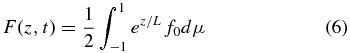
We calculated time-dependent density profiles F(z, t) by binning the particles with any pitch-angle cosine μ in a given position interval between z and z + Δz, and we compared the resulting density profiles with the theoretical predictions of the diffusion approximation. Specifically, the solution of Equation (7) with a delta-functional initial condition is given by a moving pulse
where the parameters u and κ|| are defined by Equation (8), and either Equation (9) or Equation (11) in dimensionless form.
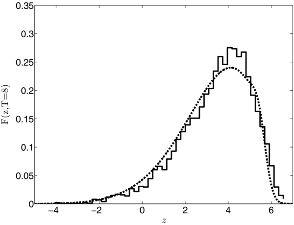
The transport coefficients calculated by Beeck & Wibberenz (1986) and by Shalchi (2011) coincide in the case of no focusing, when ξ = 0, κ||, 0 = 1/3 and u = 0. Figure 1 shows an excellent agreement between the analytical solution of Equation (17) (black curve) and numerical results (histogram) in the case of no focusing at time t = 8. The numerical results are obtained by solving Equations (15) and (16) with 106 particles and time step Δt = 0.004. The close agreement reinforces the results of the earlier numerical studies of diffusive particle transport, performed by Kóta et al. (1982). We also confirmed that the diffusion approximation remains accurate at t = 15.
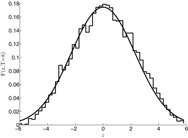
Figure 1. Analytical prediction (solid curve) and numerical results (histogram) for the density profile F(z, t) at t = 8 in a uniform mean magnetic field (ξ = 0). The numerical results are obtained by solving Equations (15) and (16) with 106 particles and time step Δt = 0.004.
Download figure:
Standard image High-resolution imageFigure 2 shows the snapshot of a moving density pulse in the case of strong focusing, ξ = 1.5. The numerical results (histogram) are obtained by solving Equations (15) and (16) with 106 particles and time step Δt = 0.004. Interesting differences among the analytical and numerical profiles emerge. The diffusive transport model of Beeck & Wibberenz (1986) (solid curve) clearly predicts the location z = ut of the peak of the pulse better than the model of Shalchi (2011; dashed curve). The model of Beeck & Wibberenz (1986) also reproduces the density profile for z < ut quite well, whereas the profile based on the model of Shalchi (2011) cannot reproduce the numerically obtained profile, even if the theoretical profile is shifted to the right to match the density peak. We confirmed that the results are similar for other values of ξ > 0 at t = 8, as well as at t = 15.
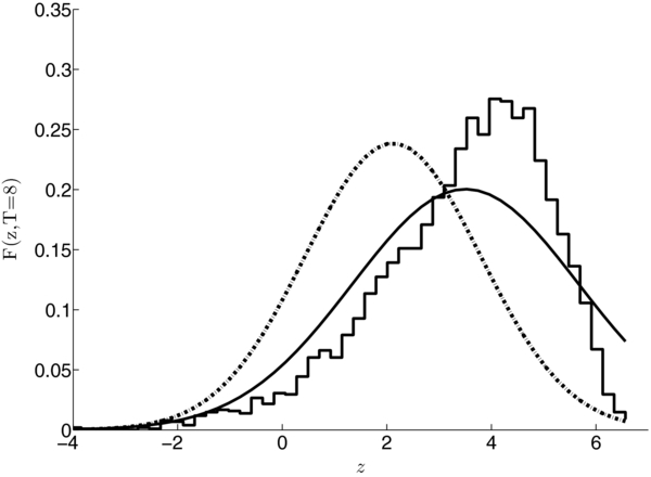
Figure 2. Analytical predictions and numerical results (histogram) for the density profile F(z, t) at t = 8 with strong focusing (ξ = 1.5). The numerical results are obtained by solving Equations (15) and (16) with 106 particles and time step Δt = 0.004. The analytical moving-pulse profiles, given by Equation (17), are based on the models of Beeck & Wibberenz (1986; solid curve) and Shalchi (2011; dashed curve).
Download figure:
Standard image High-resolution imageFigure 3 presents the dimensionless mean speed, computed from the averaged Equation (13), d〈z〉/dt = 〈μ〉, against time. For each value of time we approximate 〈μ〉 using the mean pitch-angle cosine of 106 particles. The dimensionless mean speed 〈μ〉 is plotted for ξ = 0 (points), ξ = 0.5 (crosses), and ξ = 1 (asterisks). In all cases, a constant value of 〈μ〉 is reached after a transitional period of a few scattering times.
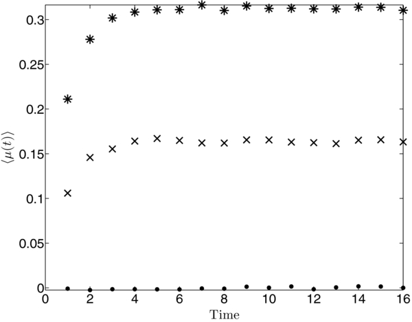
Figure 3. Dimensionless mean speed d〈z〉/dt = 〈μ〉 as a function of time. For each value of time, 〈μ〉 is computed using the mean pitch-angle cosine of 106 particles. The dimensionless mean speed 〈μ〉 is plotted for ξ = 0 (points), ξ = 0.5 (crosses), and ξ = 1 (asterisks). The transitional period of a few scattering times corresponds to the relaxation of the angular distribution to a steady distribution (see Figure 4).
Download figure:
Standard image High-resolution imageThe transitional period corresponds to the relaxation of the angular part of the distribution function f0(μ, z, t) to a steady distribution. Figure 4 presents the angular distribution computed using 106 particle simulations with ξ = 0.5. The initial uniform distribution is given (black histogram), together with the distribution at t = 2 (blue histogram) and the distribution at t = 6 (red histogram). The black curve is an exact steady analytical solution for the angular distribution, h(μ) = Aexp (ξμ) (Roelof 1969), where the normalization constant is A = ξ/2sinh (ξ). As emphasized by Litvinenko (2012b), rapid relaxation to the steady angular distribution h(μ) is a key requirement in the derivation of the diffusion approximation.

Figure 4. Angular particle distributions computed using 106 particle simulations with ξ = 0.5: the initial uniform distribution (black histogram), the distribution at t = 2 (blue histogram), and the distribution at t = 8 (red histogram). The black curve is the exact steady solution h(μ) = Aexp (ξμ) from Equation (3), where the normalization constant is A = ξ/2sinh (ξ).
Download figure:
Standard image High-resolution imageThe mean particle speed can be used as a test of the accuracy of the diffusion approximation. Figure 5 shows the dependence of the dimensionless mean speed, computed from the averaged Equation (13), on the focusing parameter ξ. For each value of ξ, we compute d〈z〉/dt = 〈μ〉 using the mean pitch-angle cosine of 106 particles at a terminal time T (black points). To allow relaxation of the angular distribution to a steady distribution, we choose a terminal time T, for each individual particle, to be uniformly distributed between 5 < T < 15. Simulations use a time step Δt = T/2000. The solid curve is the theoretical coherent speed u = ξκ||, BW due to Beeck & Wibberenz (1986), and the dashed curve is the coherent speed u = ξκ||, S due to Shalchi (2011). Figure 5 confirms that the diffusion model of Beeck & Wibberenz (1986) yields the correct value of the mean speed for the range of focusing strengths used in the simulations.
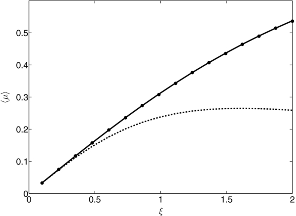
Figure 5. Limiting value of the dimensionless mean speed d〈z〉/dt = 〈μ〉 as a function of the focusing strength ξ. For each value of ξ, 〈μ〉 is computed using the mean pitch-angle cosine of 106 particles at a terminal time T. The terminal time T is taken to be uniformly distributed between 5 < T < 15. Simulations use a time step Δt = T/2000. The solid curve is the coherent speed u = ξκ||, BW due to Beeck & Wibberenz (1986), and the dashed curve is the coherent speed u = ξκ||, S due to Shalchi (2011).
Download figure:
Standard image High-resolution imageFinally, we note that the computed density profile ahead of the peak at z = ut in Figure 2 is particularly interesting. Since all particles have finite speed v, the density F(z, t) must vanish for z > vt (recall that the particle speed v = 1 in our dimensionless units). Hence the computed profile has a sharp front propagating to the right, and the particles pile up in the range ut < z < vt. Obviously these effects cannot be described by the diffusion approximation that has infinite propagation speed, and so the asymmetry of the density profile about the peak indicates the breakdown of the diffusion approximation. We return to this point in Section 3.4 below.
3.3. Distribution Variance and the Parallel Diffusion Coefficient
In order to better understand the reason for the disagreement between our numerical results and the analytical predictions of Shalchi (2011), we now investigate the variance of the particle distribution, var(z) = 〈z2〉 − 〈z〉2. On differentiating this with respect to time and using the averaged Equation (13), we get
We use the right-hand side of this equation to compute the rate of change of the variance for the evolving particle distribution.
Consider first the limit of no focusing, ξ = 0. Figure 6 shows that after a brief transitional period when the particle motion is non-diffusive, dvar(z)/2dt = κ||, 0 = 1/3, and so the variance is a linear function of time. This is a well-known result of the diffusion approximation (Kóta et al. 1982). As described above, the transitional period of a few scattering times corresponds to the relaxation of the angular distribution to a steady anisotropic distribution.
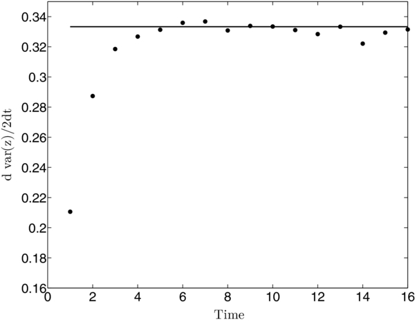
Figure 6. Dependence of the rate of change dvar(z)/2dt of the distribution variance on time for a uniform magnetic field (ξ = 0). The horizontal line is the value of the dimensionless parallel diffusion coefficient κ||, 0 = 1/3 of the diffusion approximation.
Download figure:
Standard image High-resolution imageFigure 7 shows the temporal behavior of dvar(z)/2dt in the case of strong focusing, ξ = 1.5. The solid line is the theoretical prediction κ||, BW = 0.29 due to Beeck & Wibberenz (1986), and the dashed line is the theoretical prediction κ||, S = 0.18 due to Shalchi (2011). The particle motion is initially non-diffusive, and then the variance grows linearly with time. It is clear from Figure 7 that with a high degree of accuracy dvar(z)/2dt = κ||, S after a transitional period.
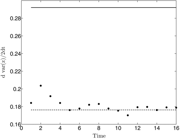
Figure 7. Dependence of dvar(z)/2dt on time for a magnetic field with strong focusing (ξ = 1.5). The solid line is the parallel diffusion coefficient κ||, BW = 0.29 due to Beeck & Wibberenz (1986), and the dashed line is the parallel diffusion coefficient κ||, S = 0.18 due to Shalchi (2011).
Download figure:
Standard image High-resolution imageFigure 8 compares the two analytical expressions for the parallel diffusion coefficient κ|| with the computed dvar(z)/2dt for 0 < ξ ⩽ 2 (standard errors are also shown). As in the calculation of the mean speed, we used the terminal time T, uniformly distributed between 5 < T < 15, and a time step Δt = T/2000. The solid and dashed curves are the dimensionless parallel diffusion coefficients predicted by Beeck & Wibberenz (1986) and Shalchi (2011), respectively. This figure confirms that dvar(z)/2dt = κ||, S for the complete range of focusing strengths (0 ⩽ ξ ⩽ 2) for which we computed the particle distributions.
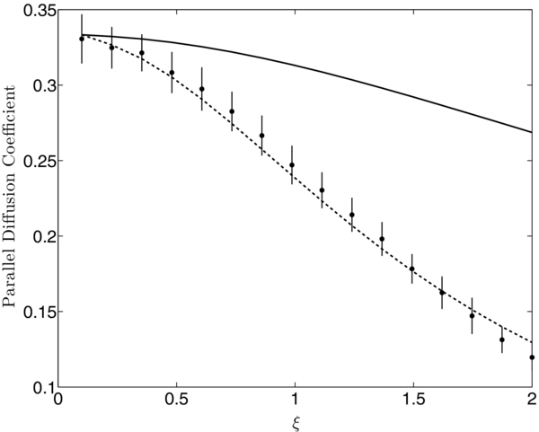
Figure 8. Limiting value of dvar(z)/2dt (with standard errors) as a function of the focusing strength ξ. For each value of ξ, the points are computed using the sample covariance of 106 simulations of μ(T) and z(T). The terminal time T and time step Δt are as in Figure 5. The solid curve is the dimensionless parallel diffusion coefficient κ||, BW due to Beeck & Wibberenz (1986), and the dashed curve is the dimensionless parallel diffusion coefficient κ||, S due to Shalchi (2011).
Download figure:
Standard image High-resolution imageOur numerical results indicate that what Shalchi (2011) calculated, at least in the case of isotropic scattering, is
This equation could serve as a correct definition of the diffusion coefficient if the diffusion approximation were sufficiently accurate for all z. As we demonstrated, however, the approximation breaks down ahead of a propagating density pulse, as a consequence of a finite particle speed. We conclude that the analysis of Beeck & Wibberenz (1986) describes correctly the location of the density maximum at z = ut and the dispersion of the cosmic-ray particles for z ⩽ ut, whereas the model of Shalchi (2011), while leading to a formally correct integral characteristic of the distribution, is physically less useful because it essentially assumes the diffusion approximation to be perfectly valid everywhere. Neither model is reliable ahead of the density pulse for z > ut where the diffusion approximation breaks down.
Interestingly, the diffusion approximation does appear to be valid for any z in the case of a uniform mean magnetic field (see Figure 1). The reason for this appears to be related to the fact that the coherent speed u vanishes when adiabatic focusing is absent. Very few particles are predicted to diffuse far from the origin in this case, which is why the resulting error is small. By contrast, strong focusing leads to a large value of the coherent speed, and as illustrated by Equation (17), the diffusion approximation predicts a much greater number of particles even far ahead of a propagating density pulse. Since this is physically impossible, in reality the particles pile up directly ahead of the density peak, creating a sharp propagating front (Figure 2).
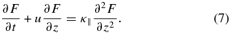
3.4. The Telegraph Equation for Particle Transport
The diffusion approximation for particle density is derived by separating the particle distribution function into the isotropic and anisotropic parts and by finding an approximate expression for the anisotropic part g = f0 − F0 (Beeck & Wibberenz 1986). When perturbation methods are used to get a more accurate expression for the anisotropic part of the distribution, the telegraph equation is obtained (Earl 1976; for alternative expansion techniques, see also Gombosi et al. 1993; Pauls & Burger 1994).
Solutions of the telegraph equation are characterized by sharp propagating fronts that resemble those in our simulations. In order to perform a detailed comparison, we use the telegraph equation
where, as before, the coherent speed u = κ||, BW/L or u = ξκ||, BW in our dimensionless variables. The telegraph equation formally reduces to the diffusion model when τ = 0. It is important to stress though that in practice τ does not vanish for any value of ξ. For instance, the reader can check that the results of Beeck & Wibberenz (1986) can be extended by obtaining a second iteration for g, which leads to τ ≈ 1 when ξ ≪ 1.
For an arbitrary focusing strength, we obtain an expression for τ in terms of ξ as follows. Equation (20) yields
On assuming that d2〈z〉/dt2 = 0 and d2var(z)/dt2 = 0 for t > τ, the equations are combined to give
Comparing this with Equation (19) yields κ||, S = κ||, BW − τu2. On substituting the expressions for κ||, BW and κ||, S from Equations (9) and (11) and solving for τ, we get
which appears to be a new result.
Figure 9 compares the numerical results (histogram) and a solution to Equation (20) (dashed curve) for the density profile at time t = 8 in the case of strong focusing, ξ = 1.5. The initial conditions for the telegraph equation are F(z, 0) = δ(z) and ∂tF(z, 0) = 0. An analytical solution of the equation in the context of focused transport is well known (Earl 1976). Since the solution is expressed in terms of special functions, however, in practice it is simpler to solve the telegraph equation numerically. We solved Equation (20) with τ given by Equation (24), using finite differences in space z and fourth-order Runge–Kutta in time (Press et al. 1986). An excellent agreement between the two density profiles strongly suggests that, wherever possible, a higher-order model should be used instead of the diffusion approximation in analysis of cosmic-ray data.
Figure 9. Solution of the telegraph equation (dashed curve) and numerical results (histogram) for the density profile F(z, t) at t = 8 with strong focusing (ξ = 1.5). The numerical results are obtained by solving Equations (15) and (16) with 106 particles and time step Δt = 0.004. The telegraph equation (Equation (20) with τ given by Equation (24)) is solved using finite differences in space and fourth-order Runge–Kutta in time.
Download figure:
Standard image High-resolution image
4. DISCUSSION
The diffusion approximation is the standard approximation for studying the cosmic-ray transport, which is why it is troubling that the expressions for the parallel diffusion coefficient κ||, derived by Beeck & Wibberenz (1986) and Shalchi (2011), are contradictory. Litvinenko (2012a, 2012b) attempted to clarify the issue by using an independent analytical method to calculate κ||. In this paper we presented the results of a complementary numerical approach to the problem.
We computed the distribution function of energetic cosmic-ray particles by solving a system of stochastic differential equations, fully equivalent to the Fokker–Planck equation, and we compared the numerically obtained evolving density profiles with analytical predictions of the diffusion approximation. In our stochastic simulations, all the particles are at z = 0 initially, corresponding to a delta-functional initial condition to the Fokker–Planck equation. The simulations strongly suggest that the key reason for the discrepancy of the analytical predictions and numerical results is that the diffusion approximation works best near and behind the peak of the particle density profile, moving with the mean speed u = κ||/L, but breaks down ahead of the peak.
We used the numerical solutions to argue that while the calculation by Shalchi (2011) appears to be mathematically correct, physically it yields a diffusion model that is less accurate than that of Beeck & Wibberenz (1986). Specifically, the model of Beeck & Wibberenz (1986) predicts more accurately both the location of the peak of a moving density pulse and the density profile behind the peak. We traced the superiority of the Beeck & Wibberenz (1986) model to its accuracy in describing the local spreading of the particles. By contrast, the model of Shalchi (2011) turns out to define the parallel diffusion coefficient in terms of the rate of change of the variance of the particle distribution. This global approach is less successful in describing the salient features of the evolving particle distribution. Thus our numerical results not only test the accuracy of the conflicting theoretical approaches, but also illustrate the important distinction between the formal correctness and physical relevance of the analytical calculations.
We also demonstrated the breakdown of the diffusion approximation ahead of the moving density pulse. Our numerical solution is characterized by a sharp propagating front and particle pile-up just ahead of the peak of the pulse, followed by a wake. These features, ultimately caused by a finite particle speed, are consistent with those of the solution of the telegraph equation, described by Earl (1976). Physically, the superior accuracy of the telegraph equation for particle density is due to the fact that its derivation takes into account higher-order terms in an expansion of the particle distribution function, which control the shape of a moving density pulse. In a new approach, we used the formula of Shalchi (2011) for the variance of the particle distribution to calculate the dependence of a coefficient in the telegraph equation on the magnetic focusing strength, and we demonstrated an excellent agreement of the solution to the resulting equation and the computed evolving profile of the density pulse. This result illustrates the usefulness of the global approach of Shalchi (2011) for particle transport studies.
Recently Tautz et al. (2012) simulated cosmic-ray transport with adiabatic focusing. They used a three-dimensional mean magnetic field and computed test-particle trajectories in a turbulent magnetic field. The computed mean free paths turned out to be much greater than the values predicted by Shalchi (2011). Tautz et al. (2012), however, did not describe the effects of coherent streaming and diffusion separately. By contrast, we used the diffusion approximation to interpret our numerical results, which enabled us to identify the separate effects of adiabatic focusing on both the parallel diffusion coefficient and the coherent speed. This is why it is difficult to compare our results and those of Tautz et al. (2012).
A more general formulation of the diffusion approximation incorporates the effects of non-isotropic scattering, magnetic helicity, and adiabatic focusing in a nonuniform large-scale magnetic field (e.g., Bieber et al. 1987; Bieber & Burger 1990; Kóta 2000; Litvinenko 2012b). It would be interesting to use the stochastic numerical techniques of this paper to investigate the accuracy of the more general diffusion approximation for the transport of energetic particles in interplanetary space, as well as generalize the telegraph equation for the particle density for a more realistic magnetic field geometry.
The authors gratefully acknowledge numerous useful discussions with Profs. I. J. D. Craig and M. S. Wheatland.