


ABSTRACT
The Large Area Telescope (LAT) on the Fermi Gamma-ray Space Telescope is a pair-conversion telescope designed to detect photons with energies from ≈20 MeV to >300 GeV. The pre-launch response functions of the LAT were determined through extensive Monte Carlo simulations and beam tests. The point-spread function (PSF) characterizing the angular distribution of reconstructed photons as a function of energy and geometry in the detector is determined here from two years of on-orbit data by examining the distributions of γ rays from pulsars and active galactic nuclei (AGNs). Above 3 GeV, the PSF is found to be broader than the pre-launch PSF. We checked for dependence of the PSF on the class of γ-ray source and observation epoch and found none. We also investigated several possible spatial models for pair-halo emission around BL Lac AGNs. We found no evidence for a component with spatial extension larger than the PSF and set upper limits on the amplitude of halo emission in stacked images of low- and high-redshift BL Lac AGNs and the TeV blazars 1ES0229+200 and 1ES0347−121.
1. INTRODUCTION
The Large Area Telescope (LAT) is the primary instrument on board the Fermi Gamma-ray Space Telescope, launched in 2008, and is sensitive to γ rays from ≈20 MeV to >300 GeV (Atwood et al. 2009). The LAT consists of a 4 × 4 array of modules called towers, each with tracker and calorimeter sections, surrounded by a segmented anticoincidence detector to veto charged particles. The tracker sections have 18 layers of alternating x–y pairs of silicon-strip detectors. Each of the first 16 layers of the tracker has a layer of tungsten foil to induce γ rays to pair convert. Pair conversion in tungsten layers in the LAT tracker creates secondary e+–e− pairs that deposit ionization energy in the silicon tracker layers. The direction of the original γ ray is reconstructed from the tracks of the secondaries, and the energy of the γ ray is determined from the energy deposition in the calorimeter and the estimated energy losses in the tracker. See Atwood et al. (2007) for further details of the tracker system.
At energies below ≈10 GeV, the accuracy of the directional reconstruction is limited by multiple scattering, whereas above ≈10 GeV, the accuracy is limited by the lever arm of the direction measurement and the 228 μm silicon-strip pitch. By design, the tracker has significantly different angular resolution depending on whether the incident γ ray converts in the front or the back tungsten layers. The 12 front conversion planes have thinner tungsten layers (3% of a radiation length) and longer track lengths for the converted pairs, yielding good angular resolution but smaller conversion efficiency. The four back conversion planes have thicker layers of tungsten (18% of a radiation length) to increase the effective area and field of view at high energies, but provide poorer angular resolution due to the increased multiple scattering and shorter track lengths.
The point-spread function (PSF) of the LAT is the probability distribution function (PDF) , for , the offset between the true () and reconstructed () directions of the γ ray of true energy E. The characteristic angular size of the PSF scales with energy as the sum of the angular uncertainties due to the instrument-pitch and multiple scattering, added in quadrature. We parameterize this energy dependence with the scaling function,


where c0 is the normalization of the multiple scattering term, c1 is instrument-pitch uncertainty, and β sets the scaling of the multiple scattering with energy. The 68% containment radius for front-converting events can be approximated with Equation (1) and c0 = 3 5, c1 = 015, and β ≈ 0.8 (Atwood et al. 2009). The angular resolution for a γ ray converting in the back layers is typically about a factor of two larger than for the front layers.
Accurate characterization of the LAT PSF is critical for proper source analysis. It has assumed additional importance because of the potential for inferring the magnitude of the intergalactic magnetic field (IGMF) BIGMF from the measurement of γ-ray halos around TeV blazars, a subset of active galactic nuclei (AGNs), e.g., Elyiv et al. (2009). In intergalactic space, BIGMF could be a remnant of exotic processes taking place in the early universe, far earlier than the decoupling epoch (Neronov & Semikoz 2009). TeV γ rays annihilating due to γ–γ interactions with the extragalactic background light (EBL) create relativistic electrons and positrons that Compton-scatter photons of the cosmic microwave background (CMB) to GeV energies. Depending on the magnitude and correlation length of BIGMF, a halo of secondary GeV photons with a characteristic spectrum (D'Avezac et al. 2007; Neronov & Vovk 2010) and angular extent (Elyiv et al. 2009) will surround a TeV source.
The MAGIC Collaboration examined several potential angular profiles of emission for the blazars Mrk 421 and 501 at energies between 0.3 and 3.0 TeV and found no significant extension compared to their PSF width of 01. The upper limit on the flux of extended emission from Mrk 501 may constrain magnetic field strengths in the range 4 × 10⁻¹⁵–1.3 × 10⁻¹⁴ G if the IGMF coherence length scale is ≳ 1 Mpc (Aleksić et al. 2010). Ando & Kusenko (2010) have recently claimed that halos around bright AGNs in LAT data give direct evidence for BIGMF ≈ 10−15 G. A subsequent analysis by Neronov et al. (2011) of the LAT data found no significant pair-halo component of AGNs when compared with the profile of the Crab pulsar and nebula. A detailed investigation of the Fermi-LAT PSF is performed in this paper using the Vela and Geminga pulsars and AGNs.
The functional representation used to characterize the PSF is described in Section 2. In Section 3, the on-orbit PSF derived from an analysis of AGNs is compared with the PSF inferred from simulations and cross-checked against an analysis of pulsars. We also consider possible contributions from systematic effects for the measured differences between the pre-launch and the on-orbit PSF. In Section 4, we present an analysis that quantifies the limits on halo emission around AGNs. Discussion and summary are given in Section 5.
2. INSTRUMENT RESPONSE AND THE POINT-SPREAD FUNCTION
To parameterize the instrument response of the LAT, we performed Monte Carlo (MC) simulations of large samples of γ rays and charged particles, and analyzed these data with our event reconstruction and classification algorithms (Atwood et al. 2009). The physical interaction of particles with the LAT is modeled by an implementation of the Gaudi73 framework and the Geant4 toolkit (Geant4 Collaboration et al. 2003), Gleam (Boinee et al. 2003). We generate a high statistics, uniform γ-ray data set using Gleam, and we apply to the events a simulation of the LAT trigger and onboard filter. Accepted events are reconstructed and undergo the same event analysis scheme as real events, the details of which may be found in Ackermann et al. (2012). The simulated particles that survive triggering and filtering are then passed through the event reconstruction and classification. The resulting MC sample was used to determine the pre-launch effective area, energy dispersion, and PSF as a function of energy and inclination angle, or the angle from the boresight (Atwood et al. 2009). A calibration unit consisting of two tracker modules and three calorimeter modules was tested with charged-particle and photon beams to validate the MC simulation (Atwood et al. 2007).
We assume azimuthal symmetry of the PSF with respect to the γ-ray direction such that the PSF can be described by a PDF with a single parameter , the angular deviation between the reconstructed and true γ-ray direction. Furthermore, we assume that the PSF does not depend on the azimuth angle of the incoming γ ray but only on the inclination angle with respect to the LAT boresight, θ. Thus the PSF can be written as P(δv; E, θ). Since the angular size of the PSF varies by two orders of magnitude over the LAT energy range, we use Equation (1) to scale out most of the energy dependence of the PSF by expressing it as a PDF in the scaled angular deviation,


We parameterize the PSF in terms of the King function (cf. King 1962), which was chosen to follow the power-law behavior of the PSF at large angular offsets. The King function has the form

and K is normalized in the small-angle approximation dΩ = xdxdϕ, so that

The parameter σ is the characteristic size of the angular distribution and γ determines the weight of the tails of the distribution. The King function becomes the normal distribution in the limit γ → ∞, where 1.51σ ≈ 68% containment. A best-fit single King function fit is not enough to properly reproduce the observed distributions of simulated γ rays (see Figure 1), so we opted for a more complex model using the sum of two King functions

where the core and tail components characterize the distributions for small and large angular separations, respectively. As can be seen from Figure 1, this functional form provides a good fit to the simulated angular distributions of event counts around the γ-ray direction. The parameters γcore and γtail determine the structure of the PSF tail and are found from simulations to decrease at high energy, yielding larger tail fractions above ≈10 GeV. For the analysis described in Section 3, we also use, as an alternative to the King function, a model independent form of the PSF parameterized by the angles corresponding to the 68% and 95% integral fractions of the distribution, or the 68% and 95% containment radii.

Figure 1. Comparison of best-fit Gaussian, single, and double King function fits to the angular distribution of simulated Diffuse-class γ rays with energy 7.5 GeV impinging at inclination angles between 26° and 37° uniformly in solid angle. The best-fit Gaussian, determined by binned likelihood, gives a poor representation of the PSF at small and large separations because of power-law tails at large angles.
Download figure:
Standard image High-resolution imageThe LAT Science Tools distribution has for each event class a set of tables that contain the PSF parameters for each conversion type (front or back) as a function of energy and inclination angle.74 By scaling out the energy dependence of the angular size σ, the tables isolate the energy dependence of the PSF tails and the weak dependence on the inclination angle. The parameters are tabulated for logarithmic energy intervals ranging from 18 MeV to 562 GeV with 4 bins per decade, and in the cosine of the inclination angle between 0.2 and 1.0 in increments of 0.1. The tables contain all of the parameters described in Equation (5) and the scaling function for the energy dependence of the σ parameters, which has the form given by Equation (1).
The PSF parameters determined from MC simulations for the pre-launch event analysis (Pass6) were the first publicly released set (e.g., Rando 2009), denoted as Pass6 version 3 (P6_V3). A range of event classifications for LAT data is available to meet different scientific requirements. The Diffuse event class selection has the highest quality requirements on track reconstruction and low charged-particle background and is most suitable for analyzing weak point sources. For these reasons, we derive the PSF for the Diffuse event class only.
Since the release of the Pass6, a newer version of the event analysis, Pass7, has been publicly released that integrates all of the known on-orbit effects into the instrument response. The PSFs associated with each of the Pass7 event classes suitable for source analysis were derived using the methodology outlined in Section 3, identical to the on-orbit PSF analysis of Pass6 Diffuse event class data. The PSFs of these event classes are described and validated in Ackermann et al. (2012).
3. ON-ORBIT PSF
The primary motivation for determining the PSF from LAT data was to verify that the reconstruction of γ rays was consistent with the simulations described in Section 2. When performing analyses of point sources using months of accumulated statistics, we noticed discrepancies between the PSF derived from MC simulations and the angular distributions of measured directions of γ rays around bright point sources with the observed distributions systematically broader for energies above a few GeV. Over time, sufficient γ-ray statistics accumulated for an accurate characterization of the on-orbit PSF at high energies. The leading considerations in the development of the on-orbit PSF for Pass6 data (P6_V11) were twofold: (1) reproducing the angular profiles of point sources in the LAT data, thereby limiting the biases and systematic uncertainties in measurements of spatial extensions and spectra of sources; and (2) smoothing the energy dependence of the PSF parameterization to avoid introducing spurious features from statistical fluctuations that could affect the quality of source analysis.
In this section we describe the stacking analysis used to determine the on-orbit PSF and the validation of the methodology using a simulation. We then verify the on-orbit PSF derived from this analysis using pulsars and AGNs. Finally, we evaluate sources of systematic uncertainties in the calibration of the instrument that may influence the PSF.
3.1. PSF Derived from Stacked AGNs
To calibrate the PSF, we adopted a technique of stacking sources, where the angular offsets of γ rays from their presumed sources are analyzed as if they came from a single source. Pulsars would be ideal for calibrating the PSF. However, the γ rays from pulsars above 10 GeV are limited, so we restrict our analysis to AGNs. A subset of 65 AGNs was selected from the Fermi-LAT First Source Catalog (henceforth 1FGL; Abdo et al. 2010b) to create a calibration sample. All the AGNs in the sample have flux between 1 and 100 GeV of at least 1.66 × 10⁻⁹ photons cm−2 s−1 and a TS75 of at least 81 above 1 GeV; a list of the sources and their properties is given in Table 1. Out of the 65 sources, 35 were associated with BL Lac-type blazars, 27 with Flat Spectrum Radio Quasars (FSRQ-type blazars), 1 with a non-blazar active galaxy, and 2 with an active galaxy of uncertain type. Though not an explicit criterion for selecting the AGN sample, the calibration sample of bright AGNs is primarily at high Galactic latitude |b| > 10°, limiting the possible systematic uncertainties associated with the background intensity and structure of the Galactic diffuse emission.
Table 1. List of AGNs from 1FGL Catalog used for Calibration of the On-orbit PSF (P6_V11)
| Source | Association | Photon Index | Fluxa | b | zc |
|---|---|---|---|---|---|
| 1FGL J0033.5−1921 | RBS 76 | 1.89 | 2.8 | 16 | 0.61 |
| 1FGL J0120.5−2700 | PKS 0118−272 | 1.99 | 3.7 | 20 | 0.557 |
| 1FGL J0136.5+3905 | B3 0133+388 | 1.73 | 4.5 | 24 | — |
| 1FGL J0137.0+4751 | OC 457 | 2.34 | 9.7 | 30 | 0.859 |
| 1FGL J0217.9+0144 | PKS 0215+015 | 2.18 | 6.0 | 25 | 1.715 |
| 1FGL J0221.0+3555 | B2 0218+35 | 2.33 | 6.4 | 26 | 0.685 |
| 1FGL J0238.6+1637 | PKS 0235+164 | 2.14 | 32.7 | 72 | 0.94 |
| 1FGL J0303.5−2406 | PKS 0301−243 | 1.98 | 4.6 | 23 | 0.26 |
| 1FGL J0319.7+4130 | NGC 1275 | 2.13 | 17.3 | 45 | 0.0176 |
| 1FGL J0334.4−3727 | CRATES J0334−3725 | 2.10 | 2.8 | 13 | — |
| 1FGL J0423.2−0118 | PKS 0420−01 | 2.42 | 5.8 | 22 | 0.916 |
| 1FGL J0428.6−3756 | PKS 0426−380 | 2.13 | 25.7 | 63 | 1.03 |
| 1FGL J0433.5+2905 | CGRaBS J0433+2905 | 2.13 | 4.5 | 16 | 0.97 |
| 1FGL J0442.7−0019 | PKS 0440−00 | 2.44 | 6.3 | 24 | 0.844 |
| 1FGL J0449.5−4350 | PKS 0447−439 | 1.95 | 11.1 | 40 | 0.205 |
| 1FGL J0457.0−2325 | PKS 0454−234 | 2.21 | 32.5 | 73 | 1.003 |
| 1FGL J0507.9+6738 | 1ES 0502+675 | 1.75 | 2.3 | 17 | 0.416 |
| 1FGL J0509.3+0540 | CGRaBS J0509+0541 | 2.16 | 3.9 | 18 | — |
| 1FGL J0538.8−4404 | PKS 0537−441 | 2.27 | 21.3 | 53 | 0.892 |
| 1FGL J0630.9−2406 | CRATES J0630−2406 | 1.87 | 3.1 | 17 | 1.238 |
| 1FGL J0700.4−6611 | PKS 0700−661 | 2.15 | 4.7 | 19 | — |
| 1FGL J0719.3+3306 | B2 0716+33 | 2.15 | 6.9 | 26 | 0.779 |
| 1FGL J0730.3−1141 | PKS 0727−11 | 2.33 | 20.7 | 44 | 1.589 |
| 1FGL J0738.2+1741 | PKS 0735+17 | 2.02 | 4.4 | 20 | 0.424 |
| 1FGL J0808.2−0750 | PKS 0805−07 | 2.14 | 10.0 | 32 | 1.837 |
| 1FGL J0818.2+4222 | B3 0814+425 | 2.15 | 8.7 | 32 | 0.53 |
| 1FGL J0825.8−2230 | PKS 0823−223 | 2.14 | 5.3 | 22 | 0.91 |
| 1FGL J0920.9+4441 | B3 0917+449 | 2.28 | 14.0 | 44 | 2.19 |
| 1FGL J0957.7+5523 | 4C +55.17 | 2.05 | 10.5 | 40 | 0.896 |
| 1FGL J1015.1+4927 | 1ES 1011+496 | 1.93 | 8.7 | 36 | 0.20 |
| 1FGL J1058.4+0134 | PKS 1055+01 | 2.29 | 7.1 | 27 | 0.888 |
| 1FGL J1058.6+5628 | CGRaBS J1058+5628 | 1.97 | 5.7 | 30 | 0.888 |
| 1FGL J1104.4+3812 | Mkn 421 | 1.81 | 26.1 | 76 | 0.03 |
| 1FGL J1159.4+2914 | 4C +29.45 | 2.37 | 5.5 | 23 | 0.729 |
| 1FGL J1221.5+2814 | W Com | 2.06 | 6.9 | 29 | 0.102 |
| 1FGL J1224.7+2121 | 4C +21.35 | 2.55 | 2.5 | 13 | 0.432 |
| 1FGL J1246.7−2545 | PKS 1244−255 | 2.31 | 8.3 | 26 | 0.635 |
| 1FGL J1248.2+5820 | CGRaBS J1248+5820 | 2.18 | 4.5 | 23 | — |
| 1FGL J1253.0+5301 | CRATES J1253+5301 | 2.14 | 3.2 | 16 | — |
| 1FGL J1256.2−0547 | 3C 279 | 2.32 | 32.4 | 72 | 0.536 |
| 1FGL J1312.4+4827 | CGRaBS J1312+4828 | 2.34 | 1.5 | 9 | 0.501 |
| 1FGL J1344.2−1723 | CGRaBS J1344−1723 | 2.11 | 6.0 | 21 | — |
| 1FGL J1426.9+2347 | PKS 1424+240 | 1.83 | 10.2 | 40 | — |
| 1FGL J1444.0−3906 | PKS 1440−389 | 1.83 | 3.5 | 16 | 0.0655 |
| 1FGL J1457.5−3540 | PKS 1454−354 | 2.27 | 16.9 | 40 | 1.424 |
| 1FGL J1504.4+1029 | PKS 1502+106 | 2.22 | 67.0 | 113 | 1.839 |
| 1FGL J1517.8−2423 | AP Lib | 2.10 | 5.6 | 21 | 0.048 |
| 1FGL J1522.1+3143 | B2 1520+31 | 2.42 | 15.9 | 48 | 1.487 |
| 1FGL J1542.9+6129 | CRATES J1542+6129 | 2.14 | 5.2 | 25 | — |
| 1FGL J1555.7+1111 | PG 1553+113 | 1.66 | 13.7 | 51 | — |
| 1FGL J1725.0+1151 | CGRaBS J1725+1152 | 1.89 | 3.4 | 16 | 0.018 |
| 1FGL J1802.5−3939 | BZU J1802−3940 | 2.25 | 10.4 | 24 | 0.296 |
| 1FGL J1903.0+5539 | CRATES J1903+5540 | 1.86 | 3.6 | 17 | — |
| 1FGL J1917.7−1922 | CGRaBS J1917−192 | 1.88 | 3.3 | 15 | 0.137 |
| 1FGL J1923.5−2104 | OV −235 | 2.17 | 11.9 | 33 | 0.874 |
| 1FGL J2000.0+6508 | 1ES 1959+650 | 2.10 | 6.0 | 26 | 0.047 |
| 1FGL J2009.5−4849 | PKS 2005−489 | 1.90 | 5.0 | 21 | 0.071 |
| 1FGL J2025.6−0735 | PKS 2023−07 | 2.35 | 12.5 | 36 | 1.338 |
| 1FGL J2056.3−4714 | PKS 2052−47 | 2.54 | 4.8 | 18 | 1.491 |
| 1FGL J2139.3−4235 | CRATES J2139−4235 | 2.08 | 8.3 | 29 | — |
| 1FGL J2158.8−3013 | PKS 2155−304 | 1.91 | 27.1 | 70 | 0.116 |
| 1FGL J2202.8+4216 | BL Lac object | 2.38 | 7.3 | 21 | 0.069 |
| 1FGL J2203.5+1726 | PKS 2201+171 | 2.39 | 4.3 | 18 | 1.076 |
| 1FGL J2253.9+1608 | 3C 454.3 | 2.47 | 46.2 | 85 | 0.859 |
| 1FGL J2329.2−4954 | PKS 2326−502 | 2.42 | 4.2 | 17 | 0.518 |

Notes. aPhoton flux between 1 and 100 GeV in units of 10−9 photons cm−2 s−1 obtained by summing the 1FGL photon flux values in the three bands from 1 to 100 GeV. bSum of the 1FGL TS values in the three bands between 1 and 100 GeV. cRedshifts for sources in 1LAC are taken from Abdo et al. (2010a). Redshifts for sources not in 1LAC are taken from the NASA Extragalactic Database (NED).
For our analysis, we used the events in the P6_V3 Diffuse class of γ rays from the 24-month period 2008 August 4–2010 August 4 (mission elapsed time in the range 239557417 s–302629417 s). We selected events with energies between 1 and 100 GeV in a region of interest (ROI) of radius 4° around each source. The lower energy limit was chosen to limit contamination in the ROIs from nearby point sources, since for the average source separation ≈70 for our sources above a Galactic latitude |b| > 10°, the 99% containment radii begin to overlap at about this energy. We also excluded events with zenith angle greater than 105° in order to limit the contamination from the Earth limb. We excluded inclination angle in the detector greater than 664 to remove γ rays for which the PSF is significantly broader and the acceptance is small (≲ 0.2% of the total acceptance). The data were split into their respective conversion types, front and back, and into four energy bins per logarithmic decade between 1 and 32 GeV and a single bin from 32 to 100 GeV. Due to the limited statistics in the energy bins above 10 GeV, the events were not binned in inclination angle. The model we derive from this analysis is representative of the PSF over exposures longer than the 53.4-day orbital precession period of the spacecraft. The PSF for a given source and observation period depends on the source observing profile, the accumulated exposure of the source as a function of its inclination angle in the LAT. Over long exposures the observing profile converges to an approximately constant shape and the use of an average PSF model is well justified. On shorter timescales, the shape of the observing profile can differ significantly and potentially introduce significant variations in the PSF relative to the one derived in this analysis.
We chose to model the angular distribution of γ rays around our sample of AGNs for a given energy bin as the sum of a single King function and an isotropic background from diffuse γ-ray emission and residual cosmic rays. The single King function parameterization was chosen over the double King function used to model the MC PSF in order to stabilize the convergence of the PSF parameters when fitting to the lower statistics of the stacked AGN sample. The log-likelihood log L for the model of the stacked counts distribution for each energy bin given the observations is defined as

where K is the normalized King function from Equation (3) as a function of angular separation xj, I is the isotropic normalization factor, and j is summed over the number of γ rays N. The localization uncertainty in the 1FGL positions was orders of magnitude smaller than the PSF, so we used the measured positions as the reference directions to determine the γ-ray angular separations.
While the King function parameter σ of the PSF has the same scaling with energy as the characteristic angular size of Equation (1), the tail parameter γ has a more complicated energy dependence. Because small changes in γ can induce large changes in the shape of the PSF, we chose to reparameterize the King function in terms of the 68% and 95% containment radii, R68 and R95. For a single King function (see Equation (3)) any two containment radii uniquely determine the parameters σ and γ. While σ and γ cannot be expressed analytically in terms of the two containment radii, they can nonetheless be determined numerically and we denote them as σ(R68, R95) and γ(R68, R95). We model the energy dependence of the 68% and 95% containment radii with two independent scaling functions, R68(E) and R95(E), with the form given by Equation (1) and each with three independent parameters: c = {c0, c1} and β.
We used a maximum likelihood analysis to determine the best-fit parameters for R68(E) and R95(E) by maximizing the sum of the log-likelihoods from Equation (6) over all the energy bands. The joint log-likelihood log L is defined as

where log L is the log-likelihood from Equation (6), is the set of angular separations in energy bin i, Ei is the bin energy, and the parameter dependence of R68(E) and R95(E) is implied. Given the best-fit scaling functions, we extract the King function parameters for the on-orbit PSF tables by evaluating σ(R68(E), R95(E)) and γ(R68(E), R95(E)) at the geometric mean energy of each bin. This procedure creates a set of PSF parameters that are smoothly varying with energy. The resulting parameterization is an extrapolation of the PSF outside the energy range of the analysis: below 1 GeV and above 100 GeV. Figure 2 compares the MC (P6_V3) and on-orbit (P6_V11) PSFs.


Figure 2. Comparison of 68% (solid lines) and 95% (dashed lines) containment radii of the MC (black) and on-orbit (green) PSF models for front- (left) and back-converting (right) Diffuse-class events.
Download figure:
Standard image High-resolution imageTo examine the potential bias of determining the PSF from on-orbit data, specifically the extrapolation of the PSF beyond the 1–100 GeV range, we generated and analyzed a detailed simulation of the sky. We simulated all sources from the Fermi-LAT Second Source Catalog (2FGL; Nolan et al. 2012), along with the Galactic and isotropic diffuse models, using the Science Tool gtobssim with the P6_V3 Diffuse PSF. The simulation covered the same time span as the on-orbit data selection and used the same cuts on inclination angle, energy, and zenith angle. We chose to use the 2FGL catalog for the simulation to account for the presence of sources not in the 1FGL that could introduce structured background and create a systematic uncertainty in the PSF determination. We analyzed the simulation with the same set of 65 AGNs from the on-orbit PSF analysis and determined the simulation PSF in the same manner as the on-orbit data, using Equation (7). The 68% and 95% containment radii determined by the PSF analysis of the simulated data are compared with those derived numerically from the P6_V3 PSF in Figure 3. The P6_V3 containment radii were derived by averaging the PSF model over inclination angle weighted by the effective area. We find good agreement between the 68% and 95% containment radii of the P6_V3 PSF and the containment radii derived from the sky simulation. Additionally, we find the containment radii extrapolated below 1 GeV and above 100 GeV are in good agreement with the measured values at these energies. This finding is consistent with the expectation from Equation (1) that the containment should follow the E−β scaling from multiple scattering below 1 GeV and take a constant value above 100 GeV.

Figure 3. 68% (open circles) and 95% (black diamonds) PSF containment radii inferred from applying the on-orbit PSF analysis to a simulated AGN sample (stack) with the properties of the calibration AGN sample generated with the P6_V3 Diffuse PSF for front- (left) and back-converting (right) events. The solid lines show the containment radii predicted by the same PSF used to generate the simulation.
Download figure:
Standard image High-resolution imageWe determined that there were no large systematic uncertainties from the determination of the PSF by the stacking technique. However, we sought to verify the on-orbit PSF using a different technique and class of point sources. The Vela and Geminga pulsars are the brightest persistent γ-ray point sources in the 100 MeV−10 GeV energy range and are alternate calibration sources for the PSF. In the next section, we use these pulsars to cross-check against the PSF inferred from AGNs, including the extrapolation below 1 GeV.
3.2. On-orbit PSF Verification
We verified the MC (P6_V3) and on-orbit (P6_V11) PSF models for the Diffuse event class with the angular distributions of γ rays from the pulsars Geminga (PSR J0633+1746) and Vela (PSR J0835−4510). The γ-ray sample was divided into four logarithmic bins per decade in energy and also separated into front and back conversion types. For each energy bin and conversion type, on- and off-pulse angular distributions were created from the pulsar data sample by selecting events with pulse-phase ranges given in Table 2. Pulse phases for the Vela pulsar were determined by using radio ephemerides derived from timing with the Parkes telescope (Weltevrede et al. 2010) and the pulse phases for the Geminga pulsar were determined from Fermi data (Abdo et al. 2010d). The pulse phases were applied to LAT data with the TEMPO2 application (Hobbs et al. 2006).76 Light curves for Vela and Geminga can be seen in Figure 4. The background in the on-pulse distributions was estimated by scaling the off-pulse distributions by the ratio of the widths of the on- and off-pulse phase intervals. The angular distribution of γ rays from a point source was then inferred as the differences by angular bin of the on- and scaled off-pulse counts distributions. This technique should provide a perfect subtraction of any unpulsed sources of γ-ray emission such as would be associated with a pulsar wind nebula (PWN) or the Galactic diffuse emission. The Vela-X PWN, a spatially extended source that is offset from the Vela pulsar by ∼1°, is approximately 500 times fainter than the Vela pulsar at 1 GeV (Abdo et al. 2010c). No evidence for a PWN has been found associated with the Geminga pulsar (Ackermann et al. 2011).

Figure 4. Light curve for all γ rays above 100 MeV within 4° of the Vela pulsar (above) and Geminga pulsar (below) in 100 fixed-count phase bins. The on- and off-pulse phase selections are identified in gray and black, respectively.
Download figure:
Standard image High-resolution imageTable 2. On- and off-pulse Phase Selection for Vela and Geminga Pulsars
| Source | On-pulse | Off-pulse |
|---|---|---|
| Vela (PSR J0835−4510) | 0.1–0.15, 0.5–0.6 | 0.7–0.1 |
| Geminga (PSR J0633+1746) | 0.1–0.17, 0.6–0.68 | 0.25–0.55 |
Download table as: ASCIITypeset image
Above 10 GeV where the statistics in the pulsar data set are limited, a comparison was made with the same high-latitude AGN sample that was used to derive the on-orbit PSF model. For the stacked AGN sample, the background was estimated by assuming an isotropic intensity determined by the events in the annulus of angular radius range 15–30 centered on the stacked 1FGL coordinates of the blazars. The 68% and 95% containment radii for the events in each energy bin were measured from the cumulative distribution of the excess. The statistical errors on the containment radii derived from both pulsars and stacked AGNs were estimated from the dispersions of containment radii determined from a large sample of MC realizations for the signal and background distributions.
Tables 3 and 4 give the 68% containment radii for front and back events estimated from Geminga and Vela below 31.6 GeV and the AGN calibration data set above 3.16 GeV. For comparison, the exposure and spectrally weighted PSF model prediction for the P6_V3 and P6_V11 PSFs are shown for a source with the observing profile of Vela and a power-law energy distribution (dN/dE∝E−Γ) with a photon index of Γ = 2. Although the effective PSF depends on the observing profile, for observations that span a time period many times greater than the orbital precession period of the LAT (53.4 days), which is the case for this analysis, the effective PSF model has only a weak dependence on the source location on the sky and is primarily a function of declination. In the energy range 100 MeV–100 GeV, the largest difference between the 68% containment radii calculated from the P6_V3 PSF using the observing profiles of Vela and the stacked AGN sample is 2%, and we therefore assume that the differences in the observing profiles of the calibration data sets can be ignored for the purposes of these comparisons. We find that the AGNs and pulsar data sets analyzed here give consistent estimates of the PSF size as a function of energy. The agreement between the containment radii inferred from Geminga and Vela validates the approach of using the off-pulse events to define the background.
Table 3. 68% Containment Radii (degrees) of the LAT PSF for Front Events in the Diffuse Class as a Function of Energy Bin Inferred from Different Calibration Data Sets: Vela, Geminga, and the AGN Calibration Sample
| Energy Bin | Vela | Geminga | AGNs | P6_V3 | P6_V11 |
|---|---|---|---|---|---|
| [log10(E/MeV)] | |||||
| 2.00–2.25 | 2.62 ± 0.06 | 2.2 ± 0.2 | ... | 2.77 | 2.99 |
| 2.25–2.50 | 1.94 ± 0.02 | 2.02 ± 0.09 | ... | 1.88 | 1.96 |
| 2.50–2.75 | 1.24 ± 0.01 | 1.25 ± 0.03 | ... | 1.21 | 1.23 |
| 2.75–3.00 | 0.771 ± 0.008 | 0.78 ± 0.01 | ... | 0.754 | 0.763 |
| 3.00–3.25 | 0.48 ± 0.005 | 0.483 ± 0.008 | ... | 0.466 | 0.481 |
| 3.25–3.50 | 0.313 ± 0.004 | 0.301 ± 0.005 | ... | 0.300 | 0.309 |
| 3.50–3.75 | 0.205 ± 0.004 | 0.212 ± 0.006 | 0.188 ± 0.005 | 0.201 | 0.209 |
| 3.75–4.00 | 0.173 ± 0.009 | 0.20 ± 0.01 | 0.168 ± 0.006 | 0.139 | 0.154 |
| 4.00–4.25 | 0.15 ± 0.01 | 0.13 ± 0.02 | 0.137 ± 0.008 | 0.0984 | 0.128 |
| 4.25–4.50 | 0.11 ± 0.02 | 0.19 ± 0.07 | 0.113 ± 0.007 | 0.0723 | 0.116 |
| 4.50–4.75 | ... | ... | 0.088 ± 0.009 | 0.0576 | 0.112 |
| 4.75–5.00 | ... | ... | 0.08 ± 0.01 | 0.0516 | 0.110 |
Notes. The containment radius of a source with the observing profile of Vela and a power-law energy distribution with a photon index Γ = 2 calculated with the P6_V3 and P6_V11 PSFs is shown for comparison.
Download table as: ASCIITypeset image
Table 4. Same as in Table 3, but for Back Events
| Energy Bin | Vela | Geminga | AGNs | P6_V3 | P6_V11 |
|---|---|---|---|---|---|
| [log10(E/MeV)] | |||||
| 2.00–2.25 | 4.7 ± 0.1 | 5.0 ± 0.5 | ... | 4.74 | 5.04 |
| 2.25–2.50 | 3.29 ± 0.04 | 3.2 ± 0.1 | ... | 3.21 | 3.38 |
| 2.50–2.75 | 2.12 ± 0.02 | 2.1 ± 0.05 | ... | 2.09 | 2.18 |
| 2.75–3.00 | 1.35 ± 0.01 | 1.41 ± 0.03 | ... | 1.31 | 1.40 |
| 3.00–3.25 | 0.88 ± 0.01 | 0.89 ± 0.01 | ... | 0.822 | 0.911 |
| 3.25–3.50 | 0.59 ± 0.01 | 0.6 ± 0.01 | ... | 0.525 | 0.613 |
| 3.50–3.75 | 0.412 ± 0.009 | 0.44 ± 0.01 | 0.40 ± 0.02 | 0.347 | 0.440 |
| 3.75–4.00 | 0.37 ± 0.02 | 0.34 ± 0.02 | 0.36 ± 0.02 | 0.240 | 0.344 |
| 4.00–4.25 | 0.37 ± 0.05 | 0.29 ± 0.04 | 0.30 ± 0.02 | 0.175 | 0.299 |
| 4.25–4.50 | 0.3 ± 0.2 | 0.5 ± 0.3 | 0.19 ± 0.02 | 0.136 | 0.278 |
| 4.50–4.75 | ... | ... | 0.19 ± 0.03 | 0.113 | 0.269 |
| 4.75–5.00 | ... | ... | 0.23 ± 0.05 | 0.101 | 0.265 |
Download table as: ASCIITypeset image
Figures 5 and 6 compare the PSF containment radii inferred from Vela and the AGN calibration data sets as a function of energy with the containment radii given by the P6_V3 and P6_V11 PSFs for front and back events, respectively. The residuals of both PSFs in the 68% containment radius are less than 10% below 3 GeV for both event classes. Above 3 GeV the MC PSF model (P6_V3) begins to significantly underpredict the size of the 68% containment radius of both front and back events. The on-orbit PSF model (P6_V11) provides an improved representation of the 68% containment radius at high energies with residuals less than 20% but overpredicts the 95% containment radius for back events. We attribute the P6_V11 back residual to using the single King function parameterization, which can overestimate the 95% containment radius of the PSF (see, for example, Figure 1).

Figure 5. Containment radii for front-converting Diffuse-class events as determined from the angular distributions of Vela and the stacked AGN sample. The blue and red curves show the 68% and 95% containment radii, respectively, given by the model predictions for the P6_V3 (solid curve) and P6_V11 (dashed curve) PSFs. PSF model predictions are shown for an observing profile corresponding to the Vela pulsar and a power-law energy distribution with photon index Γ = 2. The middle and lower panels show the fractional residuals of the 68% and 95% containment radii of Vela, the stacked AGN sample, and the P6_V11 PSF relative to the P6_V3 PSF.
Download figure:
Standard image High-resolution image
Figure 6. Same as for Figure 5, but for back-converting events.
Download figure:
Standard image High-resolution image3.3. Systematic Uncertainties in Modeling the LAT PSF
Although the reason for the discrepancy between the on-orbit (P6_V11) and MC (P6_V3) PSFs at high energies is not fully understood, we argue that it is not due to intrinsic broadening of the γ-ray distributions around the AGN sample that was used for calibration. Above 3 GeV the discrepancy in the 68% containment is 01–02 for back events but <01 for front events (see Tables 3 and 4). Given that the front PSF is approximately two times narrower than the back PSF, this discrepancy cannot be self-consistently modeled as an intrinsic spatial extension convolved with the LAT PSF. Furthermore, in the intermediate energy range (3–30 GeV) where the PSF can be independently measured using both pulsars and AGNs, the PSF containments inferred from pulsars are found to be consistent with those inferred from AGNs (see Tables 3 and 4). We therefore conclude that the majority of the PSF discrepancy can be attributed to systematic uncertainty in modeling the LAT.
We considered the residuals in the boresight alignment as a potential source of systematic uncertainty. The boresight alignment of the LAT is the orientation of its coordinate system with respect to the spacecraft coordinate system. The spacecraft determines its orientation with a pair of star trackers with an accuracy of a few arcseconds. The boresight alignment of the LAT is determined from analysis of bright point sources accumulated over several months (Abdo et al. 2009). We determined the boresight alignment early on in the mission, and the magnitude was measured to be 015 and has been monitored on weekly and monthly bases for the entire time range of the data considered here. The fluctuations are less than 0005 in a month. Therefore we rule out variations in the boresight alignment as contributing to the broadening of the on-orbit PSF relative to the MC PSF.
In the LAT event reconstruction software (Atwood et al. 2009), positional and directional information from the Calorimeter (CAL) detector system is used to seed the pattern recognition analysis that is applied to track candidates recorded by the Tracker (TKR) detector system. Furthermore, the vector from the centroid of the energy deposition in the CAL to the estimated γ-ray conversion point is considered as an additional constraint on the direction of the incoming γ ray above ∼1 GeV. The calculation of position information from the CAL relies on accurate maps of the scintillation response of the CAL crystals (Atwood et al. 2009; Grove & Johnson 2010). The response maps used to produce the Pass6 data release were derived prior to launch using cosmic-ray muons.
We identified the crystal response maps as a possible source of the discrepancy between the observed and simulated PSF at high energies, either because of a time dependence in the crystal response or because of an inaccuracy of the maps in representing the actual spatial dependence of the crystal response. To evaluate whether the PSF discrepancy was changing with time, we determined the 68% and 95% containment radii for each of the energy bins in Section 3.1 in six five-month intervals. We detected no significant changes in the containment radii in the energy range 1–32 GeV for either conversion type. Over the same time interval, however, on-orbit radiation damage to the scintillating crystals caused a typical decrease in scintillation light attenuation length of about 3%, which corresponds to an average position bias of 3 mm near the ends of crystals and up to 10 mm bias in the most sensitive crystals. Because the PSF did not show a detectable change with time, we conclude that time dependence in the crystal response is not the dominant source of the PSF discrepancy.
To test whether inaccuracy in the response maps could be the cause, we reanalyzed the sea-level and on-orbit cosmic-ray calibration data to derive maps that more closely describe the response near the end of each crystal. Using the revised response maps, we repeated the event reconstruction for a test data set consisting of events from five AGNs from the calibration sample at high latitude toward directions with low intensities of Galactic diffuse emission. For γ rays with energy greater than 5 GeV, we found that the mean angular separation from the source position in this event sample drops from 0133 ± 0004 to 0114 ± 0004. By using the improved calibration, we recovered ∼70% of the resolution loss relative to the MC expectation. We conclude, therefore, that inaccuracy in the crystal response maps used for the Pass6 event reconstruction indeed is the source of much of the PSF discrepancy. More detailed analysis and diagnosis is in progress.
4. PAIR-HALO ANALYSIS
As discussed in Section 1, the IGMF broadens the angular extent of γ-ray emission from AGNs into pair halos through the deflection of electromagnetic cascades. In contrast, the pulsed γ-ray emission from any pulsar appears as a true point source to the LAT and the pulsar emission can be effectively separated from the background of any surrounding nebula and of the diffuse interstellar and extragalactic emission through the phase-based background subtraction technique described in Section 3.2. In the following sections, we place limits on the angular extension of AGN emission relative to pulsar emission and present an analysis that evaluates the significance of two extended angular profiles for BL Lac blazar populations and TeV sources, using pulsars as calibration sources.
4.1. Maximum Likelihood Analysis in Angular Bins
To test for the presence of pair halos around AGNs, we use a joint likelihood for the angular distributions of γ rays around AGNs and pulsars. The events are binned into three logarithmic energy intervals from 1 to 31.6 GeV. Additionally, the sample is binned in angular offset from their presumed source such that there are an equal number of counts in each of 12 angular bins for the on-pulse counts from the Vela pulsar. Since the Vela pulsar emission is an order of magnitude brighter than the background intensity in the on-pulse phase, this choice of binning ensures that the integrated efficiency in each bin and thus the point-source statistics are roughly the same for all sources in each angular bin. The front-converting events have lower rates of residual cosmic rays and better angular resolution than the back events, and therefore we limit the analysis to these events.
We used a non-parametric representation of the PSF given by the fraction of events (mi) in each of the 12 angular bins, providing a more direct comparison between the pulsar and AGN angular distributions by removing any dependence of the analysis on the choice of PSF parameterization. The model for the angular distribution of events for the on-pulse pulsar emission, νoni, is expressed as

where Npsr is the number of events attributed to the pulsar in the on-pulse phase, νoffi is the model for the number of off-pulse events in angular bin i, mi is the PSF weight in angular bin i, and α is the ratio of the width of the on- and off-pulse phase selections. We chose Vela and Geminga as calibration sources for this analysis, as these pulsars have the largest number of source γ rays above 100 MeV and weak or undetected associated nebular emission. The on- and off-pulse data samples were defined using the phase ranges from Table 2 and the angular bin ranges, counts, and models are shown in Tables 5–7.
Table 5. Statistics for the Vela and Geminga Pulsars and the Low- and High-redshift BL Lac Objects in the Energy Range 1000–3162 MeV for the Analysis in Section 4.2
| Bin Edges | Vela | Geminga | BL Lac Object (z < 0.5) | BL Lac Object (z > 0.5) | |||||
|---|---|---|---|---|---|---|---|---|---|
| (deg) | mi | νoni | noni | νoni | noni | νagni | nagni | νagni | nagni |
| 0.000–0.083 | 0.083 | 996.3 | 955 | 516.7 | 560 | 442 | 450.8 | 203 | 214.0 |
| 0.083–0.124 | 0.083 | 999.9 | 988 | 512.7 | 525 | 478 | 463.9 | 206 | 215.9 |
| 0.124–0.160 | 0.083 | 999.8 | 996 | 519.0 | 523 | 486 | 472.4 | 249 | 222.7 |
| 0.160–0.199 | 0.084 | 1000.8 | 1012 | 518.7 | 507 | 533 | 493.8 | 258 | 226.5 |
| 0.199–0.239 | 0.083 | 1000.1 | 981 | 512.2 | 532 | 514 | 502.5 | 218 | 224.4 |
| 0.239–0.283 | 0.083 | 1000.3 | 1008 | 518.0 | 510 | 508 | 519.2 | 205 | 227.0 |
| 0.283–0.336 | 0.084 | 1004.3 | 1026 | 510.3 | 488 | 601 | 570.9 | 255 | 240.5 |
| 0.336–0.406 | 0.084 | 1006.0 | 1034 | 513.9 | 485 | 667 | 648.3 | 250 | 254.4 |
| 0.406–0.493 | 0.083 | 1004.6 | 999 | 513.2 | 519 | 634 | 737.7 | 288 | 278.3 |
| 0.493–0.630 | 0.083 | 1013.6 | 995 | 513.0 | 532 | 1088 | 1076.9 | 317 | 340.5 |
| 0.630–0.875 | 0.083 | 1034.3 | 1052 | 517.9 | 500 | 1799 | 1967.6 | 496 | 524.7 |
| 0.875–4.000 | 0.082 | 1874.3 | 1902 | 765.8 | 743 | 64785 | 64631.0 | 13303 | 13279.2 |
Notes. The models for the on-pulse selection νoni are displayed next to the number of counts noni in each angular bin. The BL Lac model counts νagni are fit for the null case (Nhalo = 0) in Equation (10).
Download table as: ASCIITypeset image
Table 6. Same as in Table 5 in the Energy Range 3162–10, 000 MeV
| Bin Edges | BL Lac Object | BL Lac Object | |||||||
|---|---|---|---|---|---|---|---|---|---|
| (deg) | Vela | Geminga | (z < 0.5) | (z > 0.5) | |||||
| mi | νoni | noni | νoni | noni | νagni | nagni | νagni | nagni | |
| 0.000–0.043 | 0.083 | 177.6 | 175 | 104.4 | 107 | 156 | 148.4 | 71 | 59.8 |
| 0.043–0.063 | 0.083 | 178.9 | 182 | 104.1 | 101 | 133 | 141.5 | 62 | 58.7 |
| 0.063–0.082 | 0.084 | 179.0 | 188 | 105.1 | 96 | 145 | 145.9 | 50 | 56.8 |
| 0.082–0.099 | 0.083 | 178.7 | 196 | 104.4 | 87 | 162 | 151.7 | 62 | 58.8 |
| 0.099–0.121 | 0.083 | 178.8 | 167 | 104.1 | 116 | 170 | 155.3 | 53 | 57.5 |
| 0.121–0.142 | 0.084 | 179.1 | 175 | 105.8 | 110 | 177 | 158.3 | 72 | 60.9 |
| 0.142–0.166 | 0.083 | 178.6 | 184 | 104.4 | 99 | 121 | 140.5 | 70 | 60.6 |
| 0.166–0.196 | 0.083 | 178.9 | 179 | 106.1 | 106 | 131 | 146.0 | 29 | 54.4 |
| 0.196–0.237 | 0.083 | 178.5 | 176 | 106.4 | 109 | 171 | 162.9 | 68 | 61.8 |
| 0.237–0.292 | 0.084 | 179.5 | 167 | 105.3 | 118 | 149 | 163.2 | 57 | 61.7 |
| 0.292–0.408 | 0.083 | 180.7 | 176 | 108.1 | 113 | 207 | 212.0 | 66 | 70.6 |
| 0.408–4.000 | 0.083 | 329.6 | 336 | 144.9 | 140 | 13821 | 13817.1 | 2753 | 2751.5 |
Download table as: ASCIITypeset image
Table 7. Same as in Table 5 in the Energy Range 10, 000–31, 623 MeV
| Bin Edges | BL Lac Object | BL Lac Object | |||||||
|---|---|---|---|---|---|---|---|---|---|
| (deg) | Vela | Geminga | (z < 0.5) | (z > 0.5) | |||||
| mi | νoni | noni | νoni | noni | νagni | nagni | νagni | nagni | |
| 0.000–0.026 | 0.078 | 12.1 | 12 | 3.9 | 4 | 53 | 51.6 | 9 | 10.3 |
| 0.026–0.040 | 0.088 | 13.6 | 13 | 4.4 | 5 | 61 | 59.0 | 8 | 10.7 |
| 0.040–0.051 | 0.088 | 13.6 | 11 | 4.4 | 7 | 55 | 54.6 | 17 | 14.3 |
| 0.051–0.067 | 0.088 | 13.6 | 10 | 4.4 | 8 | 62 | 59.8 | 12 | 12.3 |
| 0.067–0.077 | 0.083 | 12.9 | 13 | 4.1 | 4 | 33 | 37.4 | 16 | 13.5 |
| 0.077–0.086 | 0.088 | 13.6 | 16 | 4.4 | 2 | 44 | 46.4 | 11 | 11.9 |
| 0.086–0.104 | 0.088 | 13.6 | 14 | 4.4 | 4 | 57 | 56.2 | 11 | 11.9 |
| 0.104–0.134 | 0.088 | 13.6 | 13 | 4.4 | 5 | 72 | 67.5 | 23 | 16.9 |
| 0.134–0.164 | 0.088 | 13.6 | 17 | 4.4 | 1 | 43 | 46.1 | 11 | 12.1 |
| 0.164–0.191 | 0.083 | 12.9 | 13 | 4.1 | 4 | 46 | 47.6 | 5 | 9.3 |
| 0.191–0.260 | 0.088 | 13.6 | 14 | 4.4 | 4 | 60 | 59.8 | 14 | 13.8 |
| 0.260–4.000 | 0.053 | 38.2 | 42 | 8.7 | 6 | 3195 | 3194.9 | 638 | 637.9 |
Download table as: ASCIITypeset image
The model of the angular distribution of γ rays from AGNs is the sum of three components: point-source emission, a uniform background, and extended (halo) emission. It is given by

where Nagn is the total number of events attributed to the AGN, Niso and bi are the total number and fraction of events in angular bin i for the isotropic model. Nhalo and h*i(θ0) are the total number and fraction of events in angular bin i for the halo model, hi, convolved with the PSF. The isotropic fractions, bi, were calculated from the fraction of solid angle in the ROI contained in angular bin i. For the halo models tested in this work, hi has a single parameter, θ0, corresponding to a characteristic halo size. We convolved the halo model with a single King function that was fit to the PSF weights in the null halo case.
Given the observations , and corresponding to the on- and off-pulse pulsar and AGN counts in each of the 12 angular bins, the joint likelihood for the stacked pulsars and AGNs is


where

is the log-likelihood for observing n events given a model amplitude ν. The maximum likelihood estimators of the model parameters were evaluated by maximizing the joint likelihood with respect to all model parameters given the data.
Various models for the angular profile of halo emission induced by the IGMF have been considered (Elyiv et al. 2009; Ando & Kusenko 2010; Aleksić et al. 2010). Here we consider both Gaussian and Disk models; these can be expressed as

and

where both equations are normalized with the small-angle approximation, dΩ = 2πθdθ. The Disk and Gaussian models were chosen to bracket the shape of the model tested by Ando & Kusenko (2010), with the Disk and Gaussian representing the limiting cases of a sharply peaked and broad distribution, respectively. A test statistic TS for the halo models as a function of θ0 was constructed by evaluating the difference between the maximum likelihood of the halo model (L(Nhalo, θ0)) and the maximum likelihood of the null hypothesis (L(0, θ0)),

where all parameters besides θ0 are left free. Given the constraint that Nhalo > 0 and the null case is on the boundary of the parameter space (i.e., Nhalo = 0), the significance of the pair-halo component with characteristic extension θ0 is , provided that the number of events associated with the pulsars and AGNs, Npsr and Nagn, is larger than ∼20 (Mattox et al. 1996; Protassov et al. 2002).

4.2. Limits on the Pair-halo Emission of 1FGL BL Lac Sources
In the Fermi-LAT First AGN Catalog (henceforth 1LAC; Abdo et al. 2010a), 115 of the BL Lac-type AGNs have measured redshifts. The sources were split into low- and high-redshift groups defined by z < 0.5 and z > 0.5, respectively, to test for a redshift-dependent size difference, e.g., Ando & Kusenko (2010). The number of low- and high-redshift sources is 94 and 21, respectively. For the AGN, we used our two-year sample of P6_V3 Diffuse-class events, while the data for Vela and Geminga pulsars were further constrained by the time ranges of the available timing solutions, leaving 1.5 years of data for Vela and 1.4 for Geminga.
As in Section 3, for the AGN we included events in the energy range above 1 GeV to limit the contamination from nearby bright sources. The γ-ray data sets for the two redshift ranges were binned in energy with two bins per logarithmic decade. The significance of the halo component was evaluated with the likelihood defined in Equation (10), and the Gaussian and Disk halo parameters θ0 = 01, 05, and 1°. No TS larger than 0.1 (S ≈ 0.3σ) was obtained for any of the redshift sets or halo parameters, so upper limits were derived for the fraction of γ rays from the stacked sample attributable to a halo component (fhalo = Nhalo/(Nhalo + Nagn)). This finding is in contrast to the results of Ando & Kusenko (2010), who found 3.5σ significance for 05–08 extension (fhalo = 0.073) in the 3–10 GeV range for one year of LAT data for all 1FGL low-redshift AGNs (z < 0.5) using front- and back-converting events. Over the same range of energy, a halo component of this magnitude (fhalo = 0.073) and angular size is excluded at the 1.5σ and 2.7σ levels for the 05 Gaussian and Disk models, respectively. The upper limits on fhalo are summarized in Tables 8 and 9 and plotted in Figures 7 and 8. For the smallest halo size, θ0 = 01, the primary background for the halo component is the point-source γ rays and the upper limits become less constraining at low energies where the PSF is significantly broader than the halo (R68 ≃ 04 at 1–3.16 GeV). Sensitivity to the broader halo models, θ0 = 05 and 10, is limited by the isotropic background and thus the upper limits for the broader Gaussian models are less constraining for all energies.

Figure 7. 95% upper limits on the fraction of halo model γ rays from the low-redshift BL Lac objects, assuming a 01 (a), 05 (b), and 10 (c) halo.
Download figure:
Standard image High-resolution image
Figure 8. 95% upper limits on the fraction of halo model γ rays from the high-redshift BL Lac objects, assuming a 01 (a), 05 (b), and 10 (c) halo.
Download figure:
Standard image High-resolution image4.3. Limits on the Pair-halo Emission of TeV BL Lac Objects
The TeV BL Lac-type AGNs 1ES0229+200 (z = 0.140) and 1ES0347−121 (z = 0.188) are predicted to have detectable emission in the LAT energy range due to the suppression of the primary TeV γ rays from these sources by the EBL (Woo et al. 2005; Neronov & Vovk 2010; Tavecchio et al. 2010; Dermer et al. 2011). The multi-TeV primary photons are converted into leptons that scatter CMB photons to GeV energies, unless the IGMF is sufficiently strong to deflect enough secondary pairs away from our line of sight (Neronov & Vovk 2010). The blazar 1ES0229+200 provides the strongest constraint on the IGMF due to its significant TeV emission which extends to ∼10 TeV. The inferred primary spectra from synchrotron self-Compton emission are at or below the LAT sensitivity for an observation of two years, leaving the secondary processes as the primary detectable γ rays from these sources (Aharonian et al. 2007a; Dermer et al. 2011). A detection of 1ES0229+200 in Fermi-LAT data was recently reported in Vovk et al. (2012) using 39 months of data. In the two-year data set used for this analysis, which includes only front-converting events, we find no evidence for significant point-like emission from this source. We fit 1ES0229+200 and 1ES0347−121 with the PSF-convolved Disk and Gaussian models with θ0 = 01, 05, and 10 in four logarithmic energy bins between 1 and 100 GeV. In the 32–100 GeV energy bin the number of γ rays from pulsars is insufficient to provide a template for the PSF, and we therefore used low-redshift BL Lac objects to define the PSF template in this energy range. The AGN angular bin ranges, counts, and model amplitudes are shown in Table 10. Because 1ES0229+200 and 1ES0347−121 were not detected as a point source in the LAT energy band, we tested only for the significance of the halo component by setting Nagn = 0 in Equation (10).
Table 8. Summary of the 95% CL Upper Limits on the Fraction (fhalo = Nhalo/(Nhalo + Nagn)) of γ-ray Emission from Low-redshift BL Lac Objects Attributable to a Halo Component for the PSF-convolved Disk and Gaussian Halo Models
| Energy | Disk | Gaussian | ||||
|---|---|---|---|---|---|---|
| (MeV) | θhalo = 01 |
θhalo = 05 |
θhalo = 10 |
θhalo = 01 |
θhalo = 05 |
θhalo = 10 |
| 1000–3162 | 0.48 | 0.03 | 0.02 | 0.14 | 0.02 | 0.05 |
| 3162–10, 000 | 0.25 | 0.05 | 0.16 | 0.09 | 0.11 | 0.29 |
| 10, 000–31, 623 | 0.31 | 0.27 | 0.55 | 0.19 | 0.43 | 0.69 |
Download table as: ASCIITypeset image
Table 9. Summary of the 95% CL Upper Limits on the Fraction (fhalo = Nhalo/(Nhalo + Nagn)) of γ-ray Emission from High-redshift BL Lac Objects Attributable to a Halo Component for the PSF-convolved Disk and Gaussian Halo Models
| Energy | Disk | Gaussian | ||||
|---|---|---|---|---|---|---|
| (MeV) | θhalo = 01 |
θhalo = 05 |
θhalo = 10 |
θhalo = 01 |
θhalo = 05 |
θhalo = 10 |
| 1000–3162 | 0.57 | 0.05 | 0.04 | 0.23 | 0.05 | 0.09 |
| 3162–10, 000 | 0.25 | 0.07 | 0.20 | 0.12 | 0.15 | 0.35 |
| 10, 000–31, 623 | 0.56 | 0.34 | 0.61 | 0.28 | 0.50 | 0.73 |
Download table as: ASCIITypeset image
Table 10. Statistics for the Low-redshift BL Lac Objects in the Energy Range 31, 623–100, 000 MeV for the Analysis in Section 4.3
| Bin Edges | BL Lac Object (z < 0.5) | ||||
|---|---|---|---|---|---|
| (deg) | mi | Nagnmi | Nisobi | νagni | nagni |
| 0.000–0.019 | 0.076 | 20.0 | 0.0 | 20.0 | 20 |
| 0.019–0.026 | 0.080 | 21.0 | 0.0 | 21.0 | 21 |
| 0.026–0.033 | 0.080 | 21.0 | 0.0 | 21.0 | 21 |
| 0.033–0.043 | 0.084 | 22.0 | 0.0 | 22.0 | 22 |
| 0.043–0.049 | 0.080 | 21.0 | 0.0 | 21.0 | 21 |
| 0.049–0.058 | 0.080 | 21.0 | 0.0 | 21.0 | 21 |
| 0.058–0.073 | 0.080 | 20.9 | 0.1 | 21.0 | 21 |
| 0.073–0.102 | 0.083 | 21.7 | 0.3 | 22.0 | 22 |
| 0.102–0.130 | 0.079 | 20.7 | 0.3 | 21.0 | 21 |
| 0.130–0.849 | 0.161 | 42.0 | 36.0 | 78.0 | 78 |
| 0.849–2.739 | 0.058 | 15.3 | 346.7 | 362.0 | 362 |
| 2.739–4.000 | 0.058 | 15.1 | 433.9 | 449.0 | 449 |
Notes. The models for the BL Lac objects, νagni, is displayed next to the number of counts, n, in each angular bin. Nagnmi is displayed to highlight the equal statistics of the BL Lac objects in each angular bin.
Download table as: ASCIITypeset image
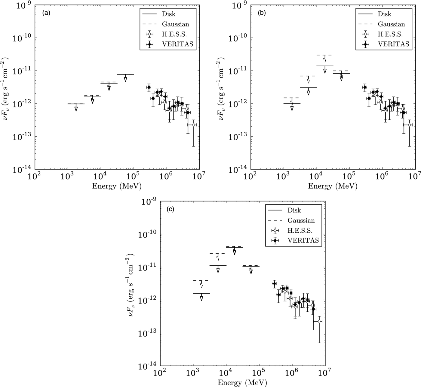
There were no detections for TS > 4(S > 2) in any energy band for either source, so we calculated the 95% upper limits on Nhalo for each source in each energy band. We converted the 95% upper limits into flux measurements by calculating the two-year exposure for each source, giving the results plotted in Figures 9 and 10 with HESS and VERITAS measurements (Aharonian et al. 2007b; Perkins & VERITAS Collaboration 2010; Aharonian et al. 2007a). We find good agreement between our upper limits and those derived by Neronov & Vovk (2010), Tavecchio et al. (2010), and Dermer et al. (2011).

Figure 9. Upper limits on the energy flux from 1ES0229+200 at the 95% confidence level assuming a 01 (a), 05 (b), and 10 (c) halo, plotted with observations from HESS and VERITAS.
Download figure:
Standard image High-resolution image
Figure 10. Upper limits on the energy flux from 1ES0347−121 at the 95% confidence level, plotted with observations from HESS assuming a 01 (a), 05 (b), and 10 (c) halo.
Download figure:
Standard image High-resolution image
5. DISCUSSION AND SUMMARY
As noted in the Section 1, TeV photons emitted by blazars can generate a secondary cascade when they pair produce on photons of the EBL and create electron–positron pairs. These pairs subsequently upscatter CMB photons through the inverse Compton process generating a secondary component of gamma-ray emission at GeV energies. By deflecting the trajectories of off-axis pairs into our line of sight, the IGMF can create a halo of cascade radiation around the blazar. The angular profile of this halo changes with the strength of the IGMF and would appear point-like within the angular resolution limit of the Fermi-LAT if the magnetic field strength is small (≲ 10−18 G). In the limit of large magnetic field strength, the cascade radiation has a maximum angular size determined by the surface subtended by the jet at a distance τ ≃ 1 from the source where τ is the pair-production optical depth of the primary very high energy (VHE) gamma rays (Neronov et al. 2010; Tavecchio et al. 2010). However, several other processes are known that could form extended emission around blazars such as synchrotron radiation from leptonic secondaries of ultra-high energy cosmic-ray (UHECR) protons undergoing photopion processes in ≫10−12 G fields (Gabici & Aharonian 2007) or cascade radiation induced by photopair losses of UHECRs (Essey & Kusenko 2010; Essey et al. 2010). Nor do halos provide the only opportunity to measure BIGMF. Combined GeV–TeV spectral analysis of moderate redshift sources (z ≈ 0.2) has already been used to infer values of BIGMF ≳ 10−15 G under the assumption of persistent blazar emission over long times (Neronov & Vovk 2010; Tavecchio et al. 2010). For blazars radiating for only a few years at a constant flux level, BIGMF ≳ 10−17 G (Dolag et al. 2011; Taylor et al. 2011) or BIGMF ≳ 10−18 G (Dermer et al. 2011) depending on the assumed unabsorbed spectrum. Searches for delayed secondary radiation from impulsive γ-ray sources provide another technique to constrain BIGMF (e.g., Plaga 1995; Murase et al. 2008).
Claims for the existence of halos around 170 stacked hard-spectrum AGNs in the 1LAC were made by Ando & Kusenko (2010) using the P6_V3 Diffuse PSF and a halo component, dN/dΩ(θ)∝exp (− θ4). This angular model is broader than the Disk model, but narrower than the Gaussian model, making it a reasonable comparison to our procedure. We attribute the detection of apparent extended emission of AGNs by Ando and Kusenko to the difference between the P6_V3 PSFs and the actual PSF as inferred here from flight data. Our results are consistent with Neronov et al. (2011) who found no evidence in the Fermi-LAT data for extended halo emission. Ando & Kusenko (2010) further claimed a detection of a halo component in the 3–10 GeV energy range using a low-redshift AGN subsample and the Crab Nebula as a PSF calibration source. In the same energy range our analysis, which used Vela and Geminga as calibration sources, set a 95% CL upper limits of 0.05 and 0.11 on the fraction of halo emission in a sample of low-redshift AGNs for a Disk and Gaussian halo models, respectively (see Table 8). Furthermore no significant detections of a halo component were found for the range of halo sizes and shapes tested.
In conclusion, we have derived the PSF through on-orbit data (P6_V11), revealing that the MC PSF (P6_V3) significantly underestimates the 68% containment radius of the PSF at GeV energies. The discrepancies are larger for back- than front-converting events with the underestimate of the 68% containment radius at 5–10 GeV reaching 25% and 50% for the two event classes, respectively. The P6_V11 PSF provides a better representation of the 68% containment radius at high energies. However, due to the limitations of the single King function parameterization that we used for P6_V11, the P6_V3 PSF more accurately describes the 95% containment radius up to ∼7 GeV. Furthermore, the P6_V11 PSF was derived from an event sample which ignored the inclination angle of the incident γ ray, and therefore does not model the dependence of the PSF on the inclination angle. The improved PSF, P6_V11, supersedes the P6_V3 PSF that has a systematically narrower model than the distributions of γ rays around bright sources. Upper limits were derived for the flux of an extended halo component in analyses of stacked AGNs. No evidence for halos around extragalactic TeV sources is found in our analysis, consistent with the limits found from other recent studies.
The Fermi-LAT Collaboration acknowledges generous ongoing support from a number of agencies and institutes that have supported both the development and the operation of the LAT as well as scientific data analysis. These include the National Aeronautics and Space Administration and the Department of Energy in the United States, the Commissariat à l'Energie Atomique and the Centre National de la Recherche Scientifique/Institut National de Physique Nucléaire et de Physique des Particules in France, the Agenzia Spaziale Italiana and the Istituto Nazionale di Fisica Nucleare in Italy, the Ministry of Education, Culture, Sports, Science and Technology (MEXT), High Energy Accelerator Research Organization (KEK) and Japan Aerospace Exploration Agency (JAXA) in Japan, and the K. A. Wallenberg Foundation, the Swedish Research Council and the Swedish National Space Board in Sweden.
Additional support for science analysis during the operations phase is gratefully acknowledged from the Istituto Nazionale di Astrofisica in Italy and the Centre National d'Études Spatiales in France.
The Parkes radio telescope is part of the Australia Telescope which is funded by the Commonwealth Government for operation as a National Facility managed by CSIRO. We thank our colleagues for their assistance with the radio timing observations.
Footnotes
- 73
Gaudi: Gaudi Project http://proj-gaudi.web.cern.ch/proj-gaudi/.
- 74
Fermi-LAT Science Tools are found at http://fermi.gsfc.nasa.gov/ssc/data/analysis/documentation/.
- 75
TS: Test Statistic, 2Δlog(likelihood) between models with and without the source, cf. Mattox et al. (1996).
- 76
Fermi pulsar ephemerides may be found at http://fermi.gsfc.nasa.gov/ssc/data/access/lat/ephems/.