


ABSTRACT
We observed Comet 29P/Schwassmann-Wachmann 1 (hereafter, 29P) in 2012 February and May with CRIRES/VLT and NIRSPEC/Keck-II, when the comet was at 6.26 AU from the Sun and about 5.50 AU from Earth. With CRIRES, we detected five CO emission lines on several nights in each epoch, confirming the ubiquitous content and release of carbon monoxide from the nucleus. This is the first simultaneous detection of multiple lines from any (neutral) gaseous species in comet 29P at infrared wavelengths. It is also the first extraction of a rotational temperature based on the intensities of simultaneously measured spectral lines in 29P, and the retrieved rotational temperature is the lowest obtained in our infrared survey to date. We present the retrieved production rates (∼3 × 1028 molecules s−1) and remarkably low (∼5 K) rotational temperatures for CO, and compare them with results from previous observations at radio wavelengths. Along with CO, we pursued detections of other volatiles, namely H2O, C2H6, C2H2, CH4, HCN, NH3, and CH3OH. Although they were not detected, we present sensitive upper limits. These results establish a new record for detections by infrared spectroscopy of parent volatiles in comets at large heliocentric distances. Until now considered to be a somewhat impossible task with IR ground-based facilities, these discoveries demonstrate new opportunities for targeting volatile species in distant comets.
Export citation and abstract BibTeX RIS
1. INTRODUCTION
In 1977, the discovery of 2060 Chiron by Charles T. Kowal drew attention to a possible distinct population of small bodies beyond Jupiter, with characteristics similar to those of known comets and asteroids. Later observational evidence led to the identification of a new dynamical class, the Centaurs, whose members are distinguished by transient orbits that cross (or have crossed) the orbits of one or more of the giant planets, and that have dynamical lifetimes of only a few million years. The current consensus is that Centaurs migrate from the Kuiper Belt (KB) or scattered disk (SD) to their current orbits after gravitational perturbation by the gas giants (Levison & Duncan 1997), but other feeding zones have been suggested as well (Volk & Malhotra 2008; Brasser et al. 2012). In a broader view, Centaurs have perihelia in the region between Jupiter and Neptune (Jewitt 2009). Those whose orbits are controlled by Jupiter are also tagged Jupiter Family Comets (JFCs), as in the case of 29P. For this reason, Centaurs are considered evolutionary links (or "transitional" members) between short-period ecliptic comets (including JFCs) and (the less modified) objects in the KB or SD.
From a sample of 23 Centaurs (including 9 "active" Centaurs), Jewitt (2009) estimated that "active" Centaurs have smaller perihelia (typically ∼5.9 AU) compared with 12.4 AU for the overall population of all known Centaurs. The proximity of Centaur comets to the Sun leads to sublimation of certain hypervolatiles (knowingly CO, although N2, S2, CH4, CO2, C2H2, and C2H6 could also sublime at these distances, if present). The low nucleus temperatures prohibit the sublimation of water and methanol in the surface layer, but icy grains can be dragged into the coma by the escaping hypervolatiles and there be warmed to sublimation temperatures or sputtered by the solar wind. The composition of the material (gas, dust, and ice) ejected from distant comets—including Centaurs—could provide an important test of possible chemical modification of gases (Stern 2003) in the surface layer of water-activated comets (i.e., those within ∼2.5 AU of the Sun). For such comets, collisions amongst chemically active species within the nucleus (e.g., acids and bases) could modify the chemical composition, causing the compositions of emergent gases and nuclear ices to differ. This comparison could reveal whether currently unrecognized chemical activity in comets measured within 2.5 AU of the Sun is biasing our emerging understanding of possible formation scenarios, and this provides strong motivation for measuring the composition of more distant comets.
Comet 29P/Schwassmann-Wachmann 1 is perhaps one of the most renowned "active" Centaur comets. It has a nearly circular orbit (eccentricity e = 0.044) just beyond that of Jupiter (semi-major axis a = 6.002 AU), and small inclination (i = 9.4°). The comet's Tisserand parameter (Tj, 2.984) places it near the border separating Jupiter-family and Centaur dynamical populations. Estimates of its rotation period are quite uncertain, varying from a few hours up to several days (e.g., Jewitt 1990; Meech et al. 1993; Stansberry et al. 2004) with recent observations in 2008 December (2009 February) returning a period of 12.1 ± 1.2 days (11.7 ± 1.5 days; Ivanova et al. 2012). Observations with Spitzer determined a nucleus radius of 27 ± 5 km (Stansberry et al. 2004), but Meech et al. (1993) claimed a radius of 8–16 km based on optical observations in 1987 August. In the optical, Jewitt (1990) confirmed a persistent dusty coma. The loss rate of dust (by mass) is nominally 300–900 kg s−1, although lower values have also been reported (Moreno 2009 and references therein).
Its particular orbital characteristics and recurrent outbursts make 29P a unique object. Thus far, the most convincing argument for the cause of its regular outbursts is the (exothermic) structural change of water ice from its amorphous to crystalline form (enabling the release of trapped, highly volatile ices such as CO) along with surface erosion (Enzian et al. 1997; Jewitt 2009). Trigo-Rodríguez et al. (2008, 2010) estimated that seven outbursts occur per year, typically with brightness increasing by 2–5 mag. It is known that water does not sublimate efficiently at large heliocentric distances (beyond about 3 AU), so carbon monoxide has been suggested as the driver of nucleus activity in 29P.
Carbon monoxide was first detected in comet 29P using radio facilities, in 1993 with JCMT (Senay & Jewitt 1994) and again in 1994 with IRAM (Crovisier et al. 1995). Estimates of production rates for CO are about (3–5) × 1028 molecules s−1 from radio observations. The lower bound corresponds to measurements by Festou et al. (2001), who indicated the possibility that 29P might have been in a rather quiescent state at the time. Several authors have suggested CO2 (which is not observable from ground-based telescopes) as another possible driver of 29P's activity, but CO2 was not detected in 29P during the Akari survey of 18 comets (the ratio of production rates in 29P at 6.18 AU heliocentric was CO/CO2 > 64, 3σ limit; Ootsubo et al. 2012). Radio observations (e.g., Senay & Jewitt 1994; Crovisier et al. 1995; Gunnarsson et al. 2008) showed an asymmetric CO emission profile with (stronger) blueshifted and (weaker) redshifted emission components that confirmed a preferentially sunward release of gas. At optical wavelengths, Cochran et al. (1991) reported detections of CO+ and CN, while Korsun et al. (2008) reported detections of CO+ and N2+.
Here, we report near-infrared spectroscopy of comet 29P in 2012 February and May. We present details of these observations and data analysis in Section 2. Section 3 deals with the modeling of carbon monoxide excitation in the coma of comet 29P, and Section 4 shows the results from our campaign. We discuss the implications of our observations in Section 5, and present our concluding remarks in Section 6.
2. OBSERVATIONS AND DATA ANALYSIS
We observed comet 29P with CRIRES (Käufl et al. 2004) at ESO's Very Large Telescope (VLT) located in the Atacama desert (Chile) on four consecutive nights (UT 2012 February 26–29, Visitor Mode). Optical observations at the Lulin Observatory indicated an increased activity of the comet on May 1 (Z. Y. Lin 2012, private communication), which triggered our observations during two consecutive nights on 2012 May 19–20 with VLT (Service Mode, using Director's Discretionary Time). On 2012 May 13, we searched for CO and H2O using NIRSPEC (AO mode) at Keck-II (McLean et al. 1998) atop Mauna Kea, Hawaii, but did not detect them.
With CRIRES, an adaptive optics module (MACAO: Multi-Applications Curvature Adaptive Optics) provided seeing correction and image stabilization, thereby delivering extremely well registered, high-resolution (λ/Δλ ∼ 5 × 10⁴) spectra of 29P. Weather conditions were favorable, with wind speeds below 5 m s−1, relative humidity below 30%, and water vapor varying from 2.2 mm to 5.8 mm during the run. Seeing was in the range of 0.5''–1.5'' in February and 0.5''–2.3'' in May. A standard star HR-4757 (T = 9900 K, mM-band = 3.02), located near the comet, allowed flux calibration and measures of column burdens for absorbing species in the terrestrial atmosphere. The CRIRES entrance slit (0 4 width) was positioned along the projected Sun–comet direction on all nights. The heliocentric distance was similar in February and May (Rh = 6.26 AU), and the solar phase angle remained small (5°–8°) during this period. The geocentric distance in February (May) was 5.44 (5.60) AU, and the relative velocity with respect to Earth was approximately −17 (+22) km s−1. The observing log and instrument settings are given in Table 1.
Table 1. Log of Observations
| Setting | Date | Time | Tia | Rhb | Rh-dotc | Δd | Δ-dote | P.A.f | αg |
|---|---|---|---|---|---|---|---|---|---|
| (UT 2012) | (UT) | (minutes) | (AU) | (km s−1) | (AU) | (km s−1) | (°) | (°) | |
| CO | February 26 | 5:06−7:43 | 120 | 6.26 | 0.05 | 5.45 | −17.0 | 305.3 | 5.5 |
| CH | " | 8:27−9:16 | 40 | " | " | 5.44 | −16.7 | " | " |
| CO | February 27 | 5:20−7:01 | 80 | 6.26 | 0.05 | 5.44 | −16.6 | 305.8 | 5.4 |
| CH | " | 7:11−9:01 | 80 | " | " | " | −16.3 | " | " |
| CO | February 28 | 5:48−7:08 | 64 | 6.26 | 0.05 | 5.43 | −16.1 | 306.3 | 5.2 |
| H2O | " | 7:15−8:02 | 40 | " | " | " | −15.9 | " | " |
| HCN | " | 8:08−9:02 | 40 | " | " | " | −15.8 | " | " |
| CH3OH | February 29 | 6:09−7:03 | 41 | 6.26 | 0.05 | 5.42 | −15.6 | 306.9 | 5.1 |
| CO | " | 7:11−9:00 | 72 | " | " | " | −15.5 | " | " |
| CO | May 13h | 5:42−7:23 | 48 | 6.26 | 0.09 | 5.52 | 19.1 | 104.9 | 6.7 |
| CO | May 19 | 1:02−2:01 | 40 | 6.26 | 0.1 | 5.60 | 21.4 | 106.8 | 7.4 |
| CH | " | 2:50−3:55 | 48 | " | " | " | 21.6 | " | " |
| CO | May 20 | 2:17−3:14 | 40 | 6.26 | 0.1 | 5.61 | 21.9 | 107.1 | 7.5 |
| CH | " | 3:23−4:27 | 48 | " | " | " | 22.0 | " | " |
Notes. The values in footnotes "b"–"g" represent the mid-point of data acquisition. aTotal on-source integration time. bHeliocentric distance. cHeliocentric velocity. dGeocentric distance. eGeocentric velocity. fPosition angle of the extended Sun–comet vector. gSolar phase (Sun–comet–Earth) angle. hObservation performed with NIRSPEC.
Download table as: ASCIITypeset image
Cometary spectra were acquired in our standard four-step sequence (ABBA) with an integration time of 60 (or 120) s per step and nodding the telescope along the slit by 15'' between the A and B positions. We followed our standard procedures for initial data reduction and analysis of the individual echelle orders (DiSanti et al. 2001; Bonev 2005; Villanueva et al. 2011b), which included flat fielding, removal of pixels affected by high dark current and/or cosmic-ray hits, spatial and spectral rectification, and spatial registration of individual A and B beams. After combining the A and B beams from the difference frames (this further assists in removing any residual background emission), we extracted spectra by summing 15 spatial pixels (1.29'') centered on the nucleus (as defined by the peak CO emission intensity).
We isolated the cometary emission lines by synthesizing a transmittance function for the terrestrial atmosphere by fitting to absorptions observed in the standard star spectra. We used a multiple layer atmosphere using the LBLRTM model (Clough et al. 2005) that accessed the HITRAN 2008 molecular database modified with our custom updates (e.g., see Villanueva et al. 2011a for details). We convolved our synthetic transmittance function to that of the comet observations, scaled it to the cometary continuum, and subtracted it from the measured spectrum. Our fluorescence models were computed at 0.1 K intervals to permit a highly accurate retrieval of the rotational temperature. Details of quantum models for each molecule can be found as follows: H2O (Villanueva et al. 2012b), C2H6 (Villanueva et al. 2011b), CH4 (Gibb et al. 2003), HCN (Lippi et al. 2013; G. Villanueva et al., in preparation), and CH3OH (Villanueva et al. 2012a). Model considerations for CO are given in Section 3.
3. MODELING OF CARBON MONOXIDE EMISSION
At infrared wavelengths, solar radiation excites (pumps) gaseous CO from rotational levels of the ground vibrational state (v = 0) to rotational levels in higher vibrational states (v = 1, 2, ...). In the absence of collisions, these excited molecular levels cascade (fluoresce) via radiative transitions (ΔJ = ±1) (eventually) to rotational levels in the ground vibrational state. For the dominant pump (the fundamental band, v = 1–0), the final ground-state (v = 0) rotational quantum numbers differ from the initial ones by 0 or ±2 units. Infrared telescopes detect the quanta released by these ro-vibrational transitions during this fluorescence process. Quantum-mechanical models estimate this spontaneous decay by determining the fluorescence efficiencies (g-factors), based on ab initio parameters (absorption line strengths, Einstein A-coefficients, statistical weights, and the total internal partition function). For our CO model, we adopted the basic line parameters given in the HITRAN 2008 Molecular Line Atlas (Rothman et al. 2009 and references therein).
Detailed pumping rates also depend on accurate determination of the incident solar infrared radiation. To approximate the flux density for the solar pump, we used a hybrid model with flux values that account for the comet's heliocentric velocity (i.e., the Swings effect; see Table 1, and Villanueva et al. 2011b for details). Differences between the hybrid model and a blackbody approximation are notorious in the 2140 cm−1 region (where the principal CO solar pump occurs), demonstrating the need for accurate determination of the solar flux as opposed to a simple blackbody approximation (Figure 1(A)). Fortunately, excellent measurements of solar spectral intensities were acquired from space at high spectral resolution (Hase et al. 2010), and these data assist in constraining the effect of solar lines in this wavelength region. Panel (B) in Figure 1 shows the good agreement between the hybrid model of Villanueva et al. (2011b) and other approximations.

Figure 1. (A) Comparison of the solar flux density using our hybrid model vs. blackbody radiator at 5770 K. (B) Comparison of the hybrid model with other methods: a semi-empirical model (Fontenla et al. 2011), and a theoretical approach (based on Kurucz 1997) and spacecraft solar data (ACE; Hase et al. 2010). We generated disk-averaged solar spectra by convolving ACE disk-center spectra with a modeled limb darkening profile (see Villanueva et al. 2011b for details). An accurate solar spectrum is essential for the calculation of fluorescence efficiencies (see Section 3). We calculated standard g-factors for a heliocentric distance of 1 AU, and then scaled them as Rh−2 to account for the distance of 29P when observed.
Download figure:
Standard image High-resolution image3.1. Boltzmann Distribution
Carbon monoxide is only weakly polar (dipole moment, 0.122 debye). Thus, radiative decay of pure rotational transitions is relatively slow compared with molecules having larger dipole moment, e.g., HCN (2.98 debye) and H2O (1.85 debye). Collisions may equilibrate rotational populations to a Boltzmann-like distribution if densities are sufficiently large, but otherwise fluorescence equilibrium may apply (Weaver & Mumma 1984; Bockelée-Morvan & Crovisier 1987). To establish the actual case using cometary data, we compare the observed fluorescent intensities with g-factors modeled for an assumed Boltzmann distribution of rotational levels in the ground vibrational state, characterized by an assumed rotational temperature (Trot). We vary Trot at regular intervals (typically 1 K for most comets, but at 0.1 K for 29P owing to its very low rotational temperature; see below) and then determine the temperature that best fits the observed line fluxes. For comets within ∼2.5 AU of the Sun, collisions dominate the rotational temperature in the near-nucleus coma, and radiative pumping of rotational levels can be neglected for typical beam sizes used at infrared wavelengths. But at ∼6 AU, our beam sizes are much larger and the collisional frequencies are much smaller. We have therefore expanded our standard treatment to include direct rotational pumping by far infrared and submillimeter photons from the 2.7 K cosmic microwave background (CMB), the cometary nucleus, and the Sun.
We modeled the excitation processes and radiative transfer in the coma, including neutral–neutral collisions, radiative pumping by solar radiation (both ro-vibrational and direct rotational pumping), and direct rotational pumping from the CMB. Relative level populations are estimated using the equation of statistical equilibrium and a radiative transfer code (based on a Monte Carlo approach; see Paganini et al. 2010 for further details).
29P is characterized by a CO-rich coma, so we expect CO–CO collisions to be significant in the inner coma, and at ∼6 AU the photodissociation lifetime (of CO) is very long (about 220 days, β = 1.9 × 10⁻⁶ s−1 at 1 AU and solar maximum; Huebner et al. 1992). Aside from CO itself, H2O and CO2 are the most abundant volatiles in most cometary comae within 2.5 AU of the Sun where they are alternative collision partners. However, these volatiles are far less abundant than CO in 29P (Bockelée-Morvan et al. 2010; Ootsubo et al. 2012), so we omit collisions with H2O and CO2. We also (arbitrarily) omit collisions with electrons from this study.
We assumed an outflow model for CO that featured steady state production with spherical symmetry and uniform outflow velocity, and calculated the radial density distribution using a production rate of 2.6 × 1028 molecules s−1, a nucleus radius of 27 km (Stansberry et al. 2004), a rotational temperature of 5 K (see Section 4.1), and a gas expansion velocity (vexp) of 0.4 km s−1 (taken from average estimates of the comet's day- and night-side velocities; Gunnarsson et al. 2008). We used theoretical cross sections (σ) to estimate the excitation of molecular rotational levels through collisions with CO and followed the standard method of assuming a cross-section that is independent of kinetic velocity (σCO−CO = 1 × 10⁻¹⁴ cm2; Biver et al. 1997; Gunnarsson et al. 2002). We estimated the effective pumping rates of rotational levels in v'' = 0 by radiative decay in excited vibrational states (v' = 1, 2, 3, and 4; including non-resonance fluorescence). See Section 3.2 for further details.
As shown in Figure 2, the model predicts an evolution from thermal to fluorescence equilibrium, with collisions controlling rotational populations in the inner coma up to a nucleocentric radius of about 104 km (for our observations, a 1'' radius corresponded to approximately 4000 km). For (steady state) spherically symmetric uniform outflow, about 64% of the total population sampled by CRIRES (field-of-view radius ∼2500 km) lies within the nucleus-centered inscribed sphere tangent to our pencil beam, and thus CRIRES is mostly sensitive to CO in the inner coma where collisions control the relative level populations. We thus expect that adopting a Boltzmann distribution in our analyses is a reasonable approximation. Of course, detailed line-by-line comparison of measured line fluxes and modeled g-factors provide a stringent experimental test of this approximation (see Section 4).
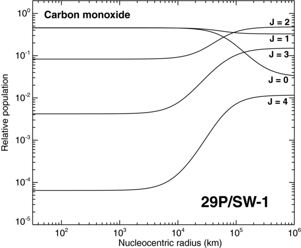
Figure 2. Estimated level populations of CO in comet 29P/Schwassmann-Wachmann 1 vs. nucleocentric distance. A radiative transfer code was applied based on a Monte Carlo approach. Details of these calculations are given in Section 3.1.
Download figure:
Standard image High-resolution image3.2. Direct Rotational Pumping by Cosmic Background and Nucleus-thermal Radiation
The CMB pervades the entire universe and is characterized by a temperature of 2.7 K. Thus, in the absence of competing cooling mechanisms, the CMB sets a lower bound to the rotational temperature of molecules in 29P. For active comets close to the Sun, inner coma rotational temperatures are much higher (40–150 K) owing to other effects (e.g., collisions) that dominate heating in the inner coma. However, at 6.26 AU, the CMB can be a controlling factor so far as rotational heating and cooling are concerned. We thus must include the CMB contribution when estimating level populations.
Heating of CO in the near-nucleus region will also occur when thermal radiation from the nucleus pumps the rotational levels directly. The nucleus of 29P is large (27 ± 5 km radius) and dark (geometric albedo = 0.025 ± 0.01; Stansberry et al. 2004). As a slow rotator (e.g., Ivanova et al. 2012), the nucleus radiates into 2π str, and at Rh ∼ 6 AU its effective surface temperature should be ∼136 K. Thus, its sub-solar temperature is estimated to be about 160 K (see Trigo-Rodríguez et al. 2008). (For comparison, the color temperature measured for coma dust in 29P at 5.73 AU was 160 K (Stansberry et al. 2004). It will be slightly cooler at 6.2 AU.) Using these parameters, we estimated the radiation field emitted by the nucleus surface and evaluated the flux density at 1000 km distance. We also calculated the thermal field from the Sun (based on a radius 6.95 × 10⁵ km, assuming a temperature of 5770 K, and Rh = 6.26 AU). The CMB is a blackbody field with effective temperature 2.7 K.
We compare the intensities of the CMB with thermal radiation from the Sun and the nucleus in Figure 3(A). Thermal emission from the Sun is dominant in the CO fundamental band region (4.7 μm, or ∼2140 cm−1), but the CMB dominates all other contributions at millimeter wavelengths (wavenumbers <15 cm−1), and thermal radiation from the nucleus prevails in the range ∼15–600 cm−1. At low frequencies, the CMB and thermal radiation from the nucleus compete significantly in determining local populations (see inset to Figure 3(A)), provided that collisions are not frequent enough to control local rotational populations. We are aware that thermal emission from coma dust could contribute to rotational pumping, however, a detailed analysis of this process is deferred to a future publication.

Figure 3. Comparison of the flux contributions of the cosmic microwave background (CMB), thermal radiation from the nucleus, and solar radiation. (A) The radiated fluxes for a wavenumber range that spans the relevant rotational and vibrational transitions in CO. Here, the thermal field radiated by the nucleus is estimated at 1000 km from the nucleus surface. Inset: we expect the CMB to be important only at very low wavenumbers (see Section 3.3) (B) Here, the wavenumber is fixed at 2140 cm−1 and the nucleocentric distance is a free parameter.
Download figure:
Standard image High-resolution imageIf we fix the wavenumber at 2140 cm−1 and analyze these contributions with respect to different nucleocentric distances, then we note that solar radiation and the nucleus contribute comparable excitation rates within the first 10 km in the coma (Figure 3(B)). At larger nucleocentric distances, solar radiation becomes the main mechanism driving most—if not all—fluorescence pumping. Considering our FOV of ∼5000 km (corresponding to the central 15 pixels in our slit), we confirm that neglecting thermal radiation by the nucleus in our analysis is a safe assumption.
3.3. Calculation of Fluorescence Efficiencies
Our CRIRES settings are sensitive to ro-vibrational transitions in the fundamental (v'–v'' = 1–0) and overtone bands (v'–v'' = 2–1, 3–2, etc.). Accordingly, we calculated g-factors for fluorescent excitation by solar radiation and subsequent decay, including cascade from the first four excited vibrational levels of CO (v' = 1 through v' = 4, see Figure 4). Direct pumping in the fundamental band (v'–v'' = 1–0) provides 98% of the total emitted energy, while cascade from v' = 2 (v'–v'' = 2–1) adds a minor contribution (∼1.8%). Cascade contributions from other vibrational levels are negligible. CO vibrational emission can also be pumped by the ultraviolet bands of the Fourth Positive Group (A1Π–X1Σg+), which has a broad Franck–Condon envelope and populates vibrational levels from v'' = 0 to v'' = 5 in fluorescent cascade (Mumma et al. 1971; Feldman & Brune 1976). However, this mechanism contributes only a minor fraction (<1%) to the total emission, and so we neglect it here. Dissociative excitation of CO2 also produces vibrationally excited CO (Mumma et al. 1971), but we also neglect this process owing to the low abundance of CO2 in 29P (Ootsubo et al. 2012). Total band g-factors are shown in Figure 4 and g-factors for individual detected CO lines are given in Table 2.
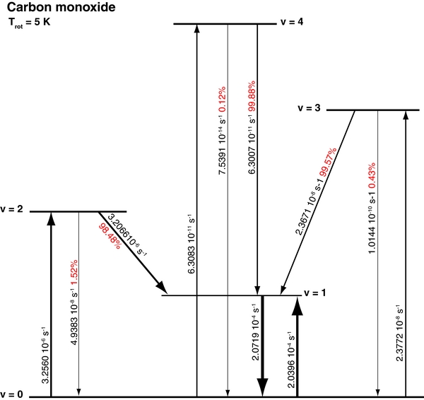
Figure 4. Band g-factors of CO at 5 K rotational temperature. Upward arrows indicate the g-factor of direct pumping of the upper level, while downward arrows indicate emission g-factors and branching rations (shown in red) into various lower vibrational levels. The fundamental vibrational band v = (1–0) is the sole band observed at infrared wavelengths, in all comets observed to date. Overtone bands have yet to be detected at infrared wavelengths, largely owing to their low emission intensities; the strongest of them (the first overtone band, v'–v'' = 2–1) is weaker than the fundamental band by a factor of ∼64. See Section 3.2 for further details.
Download figure:
Standard image High-resolution imageTable 2. Molecular Parameters for CO (v = 1–0) in 29P/SW-1
| Date | Wavenumber | g-factor | Tline | Flux | σFlux | Line Identification |
|---|---|---|---|---|---|---|
| (UT) | (cm−1) | (photons s−1 mol−1) | (W m−2) | (W m−2) | ||
| 2012 February 26–29 | ||||||
| 2150.8560 | 2.5168E−05 | 0.8635 | 2.5515E−19 | 5.6958E−20 | R 1 | |
| 2147.0811 | 3.4000E−05 | 0.8291 | 2.7254E−19 | 7.6892E−20 | R 0 | |
| 2139.4261 | 3.1880E−05 | 0.5736 | 3.5404E−19 | 7.9752E−20 | P 1 | |
| 2135.5462 | 6.6903E−05 | 0.7880 | 7.8576E−19 | 5.6573E−20 | P 2 | |
| 2131.6316 | 3.6674E−05 | 0.6982 | 4.3678E−19 | 5.3458E−20 | P 3 | |
| 2012 May 19–20 | ||||||
| 2150.8560 | 2.4655E−05 | 0.8498 | 3.2678E−19 | 1.0688E−19 | R 1 | |
| 2147.0811 | 3.7981E−05 | 0.9173 | 2.7207E−19 | 1.0171E−19 | R 0 | |
| 2135.5462 | 7.4692E−05 | 0.8782 | 9.1215E−19 | 1.1525E−19 | P 2 | |
| 2131.6316 | 3.5963E−05 | 0.8095 | 3.4951E−19 | 1.1153E−19 | P 3 | |
Note. Tline: terrestrial transmittance.
Download table as: ASCIITypeset image
4. RESULTS
We compared the calibrated flux of each ro-vibrational spectral line with correlation and excitation analyses based on quantum fluorescence models (see Sections 2 and 3). These models estimate the absolute emission g-factors for individual ro-vibrational transitions from upper state levels (v', J'), which depend on the summed pumping terms from lower state levels (v'', J''). The pumping strengths depend on the rotational temperature (Trot) of molecules in the lowest vibrational level (v'' = 0), and so are parameterized by Trot. (Here, we find it more convenient to compare measured line fluxes with models based on Trot in v' = 1.) An accurate retrieval of Trot is essential to approximate the true rotational distribution of the observed volatiles, which ultimately is required to determine precise production rates. The new fluorescence model for CO was calculated at intervals of 0.1 K, over the range 1–20 K, and the estimated fluorescence efficiencies (g-factors) agree within the experimental error with independent calculations (based on a model for CO in Villanueva et al. 2011a). The modeled cascade contributions from higher vibrational states (v' > 1, e.g., the first overtone band, v'–v'' = 2–1) are predicted to be negligible, and indeed such overtone lines are not observed in our spectra of 29P.
With CRIRES/VLT, we detected multiple CO emission lines on four nights (two nights) in 2012 February 26–29 (May 19–20). However, observations with NIRSPEC/Keck-II (with adaptive optic control) did not show evidence of CO emission on May 13. With CRIRES, we also targeted other volatiles in addition to CO (namely, H2O, C2H6, CH4, HCN, and CH3OH, see Table 1). Although not detected, we obtained upper limits, assuming release directly from the nucleus (icy grain release was not considered). Table 3 summarizes these results.
Table 3. Molecular Abundances for Primary Volatiles in Comet 29P/Schwassmann-Wachmann 1
| Species | νa | Lines | Trot | Global Qb | Abundance |
|---|---|---|---|---|---|
| (cm−1) | (K) | (1026 s−1) | (Relative) | ||
| 2012 February 26–29 | |||||
| COc | 2141.28 | 5 |  d d |
264.3 ± 34.5 | 100 |
| H2O | 3427.52 | 7 | (5.0)e | <4834.5 | <1829.1 |
| C2H6f | 2988.23 | 4 | (5.0) | <5.7 | <2.2 |
| CH4f | 3028.69 | 3 | (5.0) | <18.2 | <6.9 |
| HCN | 3305.88 | 10 | (5.0) | <13.7 | <5.2 |
| C2H2 | 3387.69 | 11 | (5.0) | <27.3 | <10.3 |
| NH3 | 3306.18 | 4 | (5.0) | <109.6 | <41.5 |
| CH3OH | 2843.25 | 6 | (5.0) | <93.2 | <35.3 |
| 2012 May 19–20 | |||||
| COg | 2141.27 | 4 |  |
268.7 ± 43.4 | 100 |
| C2H6g | 2988.25 | 4 | (5.0) | <6.8 | <2.5 |
| CH4g | 3038.50 | 3 | (5.0) | <13.0 | <4.8 |
Notes. Abundance ratios are expressed relative to CO. Uncertainties represent 1σ, and upper limits represent 3σ. The reported error in production rate includes the line-by-line scatter in measured column densities, along with photon noise, systematic uncertainty in the removal of the cometary continuum, and (minor) uncertainty in rotational temperature. aMean wavenumber of all emission lines (used for this reduction) from a particular species. bGlobal production rate, after applying a measured growth factor in CO of 1.7 ± 0.2 to the nucleus-centered production rate. (A growth factor of 1.7 is assumed for other molecules.) cThe results of Trot and Global Q for CO are based on combined observations from February 26–29. dWe tabulate the retrieved Trot and confidence limits. eWe adopted Trot = 5.0 K when calculating the NC production rates for species other than CO (whose Trot determination was not possible). This is indicated as (5.0). fResults of Global Q are based on combined observations from February 26–27. gThe results of Trot and Global Q are based on combined observations from May 19–20.
Download table as: ASCIITypeset image
4.1. Rotational Temperature
In 2012 February and May, we detected multiple CO emission lines in comet 29P, with CRIRES (Figures 5 and 6). To improve the signal to noise ratio, we combined CO observations from four consecutive nights in 2012 February, and did likewise for the two nights in May.7 This allowed robust retrievals of rotational temperatures.
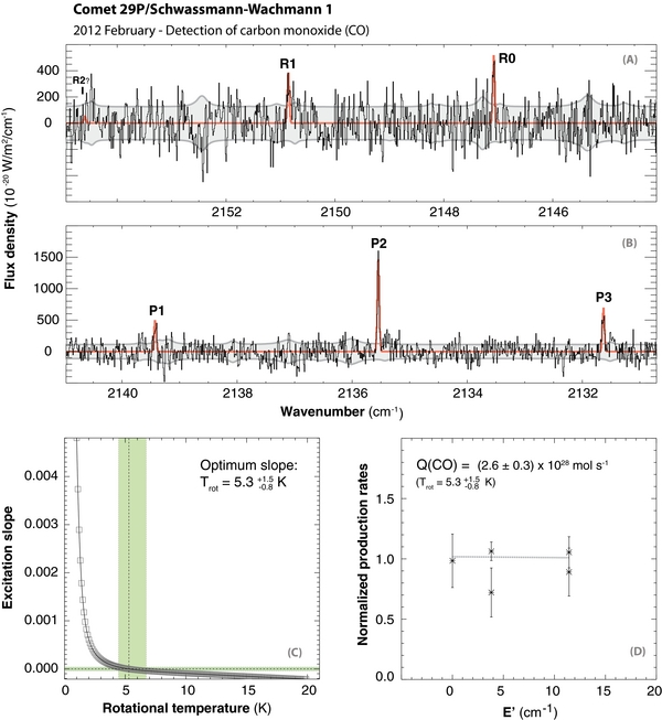
Figure 5. Emission spectra of CO (fundamental band, v = 1–0) in 29P/Schwassmann-Wachmann 1, on UT 2012 February 26–29 at resolving power 5 × 10⁴. (A) Detections of R1 and R0 emission lines in CRIRES, detector 2. (B) Detections of P1, P2, and P3 in CRIRES, detector 3. In panels A and B, the continuous (underlying) red line depicts the modeled spectra. (C) Correlation analysis, and (D) excitation analysis. In panel D, the (normalized) total production rate retrieved from each line is shown vs. the rotational energy (E', cm−1) of the emitting level (v' = 1, J'), for the best-fit rotational temperature of the upper vibrational state (v' = 1). Each line samples a specific upper level (E', J'), with P1 sampling (E' = 0, J' = 0); R0 and P2 sampling (3.8, 1), and R1 and P3 sampling (11.3, 2). From these data, we retrieved a rotational temperature of  K and a production rate of CO equal to (2.6 ± 0.3) × 1028 molecules s−1 (see Section 4).
Download figure:
Standard image High-resolution image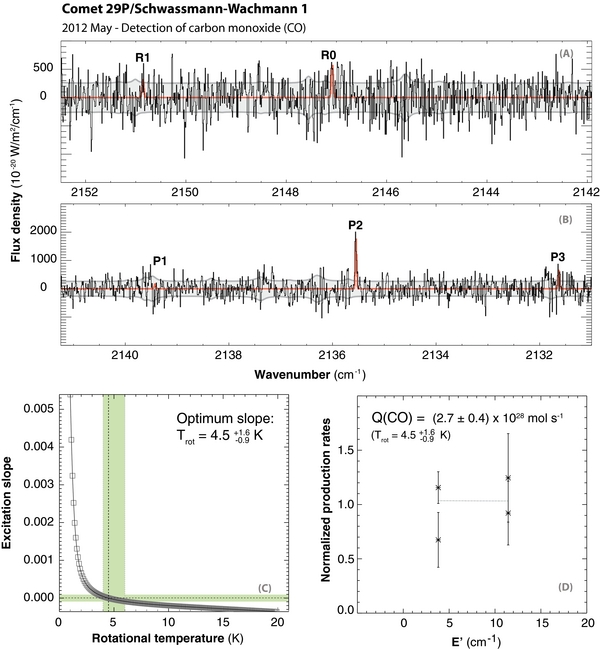
Figure 6. Emission spectra of CO (fundamental band, v = 1–0) in 29P/Schwassmann-Wachmann 1, on UT 2012 May 19 and 20. We retrieved a rotational temperature of  K and a production rate of CO equal to (2.7 ± 0.4) × 1028 molecules s−1 (see Section 4). Panels are explained in Figure 5.
Download figure:
Standard image High-resolution imageIn Figure 5, panels (A) and (B) display simultaneous detections with CRIRES in detector 2 (two lines: R0 and R1) and detector 3 (three lines: P1, P2, and P3). As shown in panels C and D, the correlation and excitation analyses led to a rotational temperature of  K.
K.
Figure 6 displays spectral detections of CO emission in May. These yield Trot =  K, slightly lower yet in good agreement (within their 1σ confidence limits) with our results from February. Our combined CRIRES results (February and May) provide a weighted mean rotational temperature of 4.9 ± 1.2 K.
4.2. Production Rates for CO
Once rotational temperatures are known, a value for the total nucleus-centered production rate (QNC) is determined from the flux of each ro-vibrational transition detected within our sampled aperture. The formalism requires a number of molecular parameters (such as the molecule's lifetime τ, the fraction of total coma content sampled for the molecule under study f(x), and fluorescence efficiencies gline at the appropriate Trot) and current astrometric parameters (e.g., geocentric distance Δ and terrestrial transmittance Tline),
However, for spherically symmetric uniform outflow, f(x) is inversely proportional to τ, making QNC formally independent of the molecular lifetime.
Accurate modeling of the terrestrial atmosphere is essential to identify and remove residual terrestrial absorptions, and also to establish the monochromatic transmittance at the Doppler-shifted position of each cometary emission line (as determined by the geocentric velocity; see DiSanti et al. 2006 and references therein).
Atmospheric "seeing" and slight aperture effects (e.g., exact positioning of the comet photocenter in the slit) cause a loss of flux ("slit losses"), and is compensated for by including a correction or growth factor (GF) that is determined from the profile of emission line intensities along the slit (i.e., the emission spatial profile; e.g., see Xie & Mumma 1996; DiSanti et al. 2001). This GF is applied to retrieved nucleus-centered production rates, resulting in total "global" production rates. The spatial profile for the binned data of February 26–29 returned a growth factor of 1.7 ± 0.2 in the retrieved production rates (Table 1 and Figure 7).8 This led to a CO production rate of (2.6 ± 0.3) × 1028 molecules s−1 in February and (2.7 ± 0.4) × 1028 molecules s−1 in May (Table 3).

Figure 7. Loss of flux (slit losses) due to atmospheric "seeing" and to slight aperture effects is compensated by a correction or growth factor (GF) determined from analyses of the gradient in emission line intensities along the slit. Due to noise constraints we applied GF = 1.7 ± 0.2 to all observations during our entire campaign of comet 29P. This profile is obtained from binned data spanning several nights on 2012 February 26–29.
Download figure:
Standard image High-resolution imageOn May 13, CO was searched for but not detected at an upper limit (3σ) of 5.8 × 1028 s−1 with NIRSPEC in AO mode (NIRSPAO). During these observations, the coma of 29P was extended (at least 5'') on the AO acquisition camera. Having a slit length of 2.26'', nodding with NIRSPAO was only 1.1'', possibly limiting our sensitivity due to cancellation of signal between beam positions. Although the AO system was stable, there were some systematic errors; we expect to address these issues in future NIRSPAO observations.
Our rotational temperatures in 2012 February and May and their mean (4.9 ± 1.2 K) are consistent with the estimate of 4 K obtained from the CO (J = 2–1) emission line alone (230 GHz; Gunnarsson et al. 2008). However, our production rates are lower by a factor of 1.3 compared to their values (∼3 × 1028 molecules s−1 versus ∼4 × 1028 molecules s−1, respectively), but are consistent with results reported by Festou et al. (2001) after applying a correction factor of 1.5 (Gunnarsson et al. 2008). Gunnarsson et al. argued that CO production in 29P can vary intrinsically by a factor of three. This is (qualitatively) consistent with observed fluctuations in optical brightness; Trigo-Rodríguez et al. (2010) reported large brightness excursions (by 2–5 mag) during outbursts. During late 2012 February, contemporaneous optical observations estimated R-magnitude ∼15.5 (Trigo-Rodríguez et al. 2012), suggesting that the comet was in a rather quiescent mode. Thus, we consider these differences in CO production to be normal, and conclude that the production rates measured in 2012 (February and May) are associated with periods of relatively quiescent activity of the comet (see Festou et al. 2001; Trigo-Rodríguez et al. 2010).
4.3. Spatial Profile
In both February and May, we oriented the slit along the extended Sun-comet projected radius vector (position angle, P.A.), equal to ∼306° in February and 107° in May (Table 1). The solar phase angle of 5°–8° indicates that the sub-solar point was placed well within the Earth-facing hemisphere.9 The distribution of CO along the slit direction is nearly symmetric about the nucleus out to nucleocentric distances beyond 4000 km but with some enhancement in the southeast direction ("+" direction on the slit), suggestive of outward flow in the sunward direction (see compass roses, Figure 8). However, because of the small phase angle, the southeast enhancement seen in our spatial profile could as well be produced by CO released into the anti-sunward hemisphere. Line-of-sight velocity measurements are needed to resolve the directionality of CO release, and they are provided by radio results. The Sun- and Earth-facing release of gas found by several radio studies confirms our hypothesis about sunward emission of the CO gas; CO emission displayed a blueshifted release during similar observational circumstances to those reported here (e.g., Senay & Jewitt 1994; Crovisier et al. 1995; Festou et al. 2001; Gunnarsson et al. 2003; Jewitt et al. 2008).

Figure 8. Spatial profiles of CO in comet 29P. This profile is obtained from binned data spanning several nights on 2012 February 26–29. The gray-shaded profile was measured for the standard star HR-4757, and is representative of the point-spread function (PSF) in our observations. See Section 4.3 for further discussion. The slit was positioned along the projected comet–Sun radius vector (P.A. ∼ 306°), and the projected sunward direction (+) and solar phase angle (5°) are marked.
Download figure:
Standard image High-resolution image
5. DISCUSSION
To date, existing observational studies of comet 29P have provided interesting perspectives on gas and dust production rates, periodicity, nucleus size, and coma morphology. However, the peculiar nature of 29P, and the sparse compositional information make it challenging to associate its chemical taxonomy with a possible formative heritage. Additional chemical constraints are clearly needed.
A similar situation occurs with most Centaurs (e.g., Bockelée-Morvan et al. 2001; Jewitt et al. 2008), whose absence of volatiles reveals either that these objects experienced significant escape of hypervolatiles (Bockelée-Morvan et al. 2001), or that the lack of significant external (solar) radiation might hinder activation mechanisms in these bodies. For instance, large efforts have been made to classify these objects into groupings based on surface colors, but no clear trend is found (Peixinho et al. 2012). The limited quantitative information regarding volatiles stems largely from three factors: (1) absence of significant activity (outgassing), (2) lack of sensitivity of some ground-based facilities, and (3) insufficient observational campaigns on distant comets in the infrared and radio.
Centaur comet 29P is a rather atypical object. In addition to its quasi-circular orbit and frequent outbursts, it is the first—and as yet the only—such comet in which CO has been detected over multiple epochs since its first detection about 20 years ago. The overall characteristics of 29P have been compared to comet C/1995 O1 (Hale-Bopp) because of their similar nucleus sizes (Weaver & Lamy 1997; Stansberry et al. 2004), emission patterns (Sekanina 1996; Gunnarsson et al. 2003), mineral content (Gehrz et al. 2006), and CO rotational temperature and production rate at Rh = 6 AU (see Biver et al. 2002; Festou et al. 2001). Carbon monoxide was the only volatile detected during our campaign, and thus we confirm CO as a key driver—perhaps the only one—controlling the observed activity. We pursued other volatiles and obtained upper limits (3σ) for seven species (H2O, C2H6, C2H2, CH4, HCN, NH3, and CH3OH). Approximate abundances in Hale-Bopp at ∼6 AU from the Sun (Biver et al. 2002) resulted in HCN/CO ∼ 0.5% and CH3OH/CO ∼ 5%, which are about an order of magnitude smaller than our upper limits in comet 29P at 6.26 AU. The capability to sample symmetric species by IR observations yielded the first estimates of the hypervolatiles C2H6 and CH4 in 29P, leading to abundances (relative to CO) of <2% and <6%, respectively.
Recently, space-based infrared observatories have provided new insights into the content and release of three major parent volatiles: H2O, CO, and CO2. The Herschel Space Observatory confirmed the detection of some water vapor (CO/H2O ∼ 10), likely from evaporation of icy grains in the coma, during the quiescent phase and two days after a major outburst (Bockelée-Morvan et al. 2010). During observations on 2009 November 18, Akari quantified the presence of H2O and abundant CO in 29P, but CO2 was not detected—the production rate ratios were CO/H2O ∼ 4.7 ± 0.3 and CO/CO2 > 64 (Ootsubo et al. 2012). Previous observations of H2O (with Odin) and CO (with IRAM) resulted in CO/H2O > 1.6 (Biver et al. 2007; Gunnarsson et al. 2008)
The large amount of carbon monoxide in 29P is significant, especially considering that the Akari survey found depleted CO in most comets sampled (Ootsubo et al. 2012). As discussed by Paganini et al. (2012b), prior to its incorporation in cometary nuclei, CO ice must have formed in outer regions of the disk after collapse of the nebular cloud, or within water-ice mantles—both shielding CO from the influence of stellar radiation. If so, then we should expect the abundance of some coeval hypervolatiles (CO, CH4, C2H6) formed in those "cold" regions. However, Spitzer observations indicated the presence of crystalline silicates in 29P's coma (Stansberry et al. 2004; Kelley & Wooden 2009). These grains must have experienced strong thermal processing (at high temperatures) very near the young Sun, for instance, like those in Oort cloud comet C/1995 O1 (Wooden et al. 1999) and in JFC 81P/Wild 2 (Brownlee et al. 2006).
Perhaps these are indicators of a duality in these small bodies, suggesting compositional heterogeneity among the comet population. We observe similar cases in other cosmogonic parameters that show no clear trend, e.g., in spin temperatures, isotopologues, dust composition (crystalline silicates), and overall chemical taxonomy (see Mumma & Charnley 2011 for a review; also the cases by Gibb et al. 2012; Paganini et al. 2012a; Bockelée-Morvan et al. 2012). Moreover, we find further evidence in recent observations of the possible presence of polar and apolar phases of ices in cometary nuclei (e.g., Villanueva et al. 2011a; Mumma et al. 2011; Paganini et al. 2012b) suggesting some heterogeneity in the nucleus. Along this line of thought, A'Hearn et al. (2012) reviewed CO and CO2 abundances relative to water in several comets, and proposed that comets formed between (or near) the CO and CO2 snow lines. The latter study also provided a possible explanation for the CO2 abundance in comets, recalling the idea of its formation from grain-surface reaction of CO ice on cold dust particles in the presence of OH radicals (Oba et al. 2010; Garrod & Pauly 2011; Noble et al. 2011).
The CO depletion in comets, however, is not fully explained. The formation of CO2 from CO ices could have been highly efficient, but, conversely, we also observe CO "enrichment" in some comets (this work; Paganini et al. 2012b and references therein)—that is not entirely consistent with this idea. We propose dynamical effects as a possible additional mechanism that could have shaped the volatile abundance in these objects. Indeed, Walsh et al. (2011) proposed that the turbulent interaction of giant planets in the first 5 Myr of our early solar system, leading to an inward-and-later-outward migration in the accretion disk, was essential in terrestrial planet formation. Taking into account a possible formation of (some) comets near the CO and CO2 snow lines, we suggest that such inward migration could have also been responsible for the depletion of the more volatile species in these bodies. Later, the turbulent outward migration (e.g., Gomes et al. 2005) ousted these small bodies to their current reservoirs.
Even though Akari has enhanced our knowledge of the carbon chemistry of comets, our understanding of it is still incomplete. Most infrared observations are performed on comets at heliocentric distances within 2–3 AU of the Sun, where water becomes fully activated and is detected through its hot-band emissions at infrared wavelengths. Carbon monoxide desorbs at 15–30 K (depending on the ice matrix composition of the nucleus) and so is one of the first hypervolatiles to sublimate as a comet approaches the Sun. In the infrared, observations of CO beyond 4 AU are few (see DiSanti et al. 1999), largely because of technical challenges, but recent detections of hypervolatiles at large Rh represent a breakthrough in ground-based infrared spectroscopy (e.g., this work; B. P. Bonev et al., in preparation10). With the advent of astronomical surveys (LONEOS, WISE/NEOWISE, PanSTARRS, LINEAR), the discovery of new distant objects has improved dramatically and, since detection of hypervolatiles at large Rh has now proven successful, timely observations of parent volatiles can reveal aspects of the composition of distant comets, the evolution of parent volatile production with heliocentric distance, and the chemistry of volatiles in comets not activated by water.
6. SUMMARY
We acquired near-infrared spectra of comet 29P/Schwassmann-Wachmann 1 in 2012 using CRIRES/VLT and NIRSPEC/Keck-II when the comet was 6.26 AU from the Sun and approximately 5.50 AU from Earth. We detected the release of carbon monoxide with similar production rates on multiple nights in epochs separated by three months, suggesting its ubiquitous release from the nucleus and thus confirming observations at radio wavelengths.
We simultaneously sampled five emission lines from a primary (parent) volatile in 29P—a "first" for this comet. From them, we retrieved very low rotational temperatures for CO ( K in February and
  K in May) that agree within their 1σ confidence limits, and also agree with the temperature retrieved from maps of radio detections of CO (J = 2–1; Gunnarsson et al. 2008). Total production rates were also in agreement: (2.6 ± 0.3) × 1028 molecules s−1 in February and (2.7 ± 0.4) × 1028 molecules s−1 in May.
Considering previous studies of CO production, we estimate our production rates to be consistent with relatively quiescent activity, or at least not consistent with periods of strong outgassing from comet 29P. Our search for other primary volatiles yielded upper limits for seven species (H2O, C2H6, C2H2, CH4, HCN, NH3, and CH3OH). Considering the ten-fold brightening that 29P undergoes during its frequent outbursts, improved constraints on their abundances (possibly including detections) should be possible in future observations.
Our results establish a new record for detections by infrared spectroscopy of parent volatiles in comets at relatively large heliocentric distances, previously held by detection of CO in C/1995 O1 (Hale-Bopp) at 4.11 AU (with CSHELL/IRTF; DiSanti et al. 1999). Until now considered to be a somewhat impossible task with IR ground-based facilities, these discoveries demonstrate new opportunities for targeting multiple volatile species at low rotational temperatures, as well as the unique possibility of characterizing hypervolatiles in distant comets.
We thank the VLT science operations team of the European Southern Observatory and the W. M. Keck Observatory for efficient operations of the observatories. L.P. acknowledges Retha Pretorius, Jonathan Smoker and Carla Aubel for their great assistance, and thanks Michael A'Hearn and Martin Cordiner for helpful discussions. We are also grateful to Zhong-Yi Lin and Josep Trigo-Rodríguez for providing magnitude estimations, and to the anonymous referee for helpful comments. This work was supported by NASA's Postdoctoral (L.P.), Planetary Astronomy (PI: M.J.M. and PI: M.A.D.), and Astrobiology Programs (PI: M.J.M.), NSF (PI: B.P.B.), the Max-Planck-Gesellschaft (H.B.), and the German–Israeli Foundation for Scientific Research and Development (H.B. and M.L.).
Footnotes
- *
Based on observations obtained at the European Southern Observatory at Cerro Paranal, Chile, under programs 088.C-0092 and 289.C-5014; and the Keck Observatory on Mauna Kea, Hawaii, under program C252ANS.
- 7
Single-night estimates of Trot and Q(CO) are in agreement (within their confidence levels), and thus we consider that binning these data was not affected by any significant short-term variations in the coma.
- 8
We applied this GF to other settings, including all observations gathered in May (due to limitations in SNR). See Table 3.
- 9
Thus, in the interpretation of our 1D spatial profile, we remind the reader that the spatial distribution is relative to this geometry.
- 10
In the IR, we also detected CO in comet C/2006 W3 (Christensen) at 4.03 AU from the Sun.