


ABSTRACT
The Q/U Imaging ExperimenT (QUIET) is designed to measure polarization in the cosmic microwave background, targeting the imprint of inflationary gravitational waves at large angular scales(∼1°). Between 2008 October and 2010 December, two independent receiver arrays were deployed sequentially on a 1.4 m side-fed Dragonian telescope. The polarimeters that form the focal planes use a compact design based on high electron mobility transistors (HEMTs) that provides simultaneous measurements of the Stokes parameters Q, U, and I in a single module. The 17-element Q-band polarimeter array, with a central frequency of 43.1 GHz, has the best sensitivity (69 μKs1/2) and the lowest instrumental systematic errors ever achieved in this band, contributing to the tensor-to-scalar ratio at r < 0.1. The 84-element W-band polarimeter array has a sensitivity of 87 μKs1/2 at a central frequency of 94.5 GHz. It has the lowest systematic errors to date, contributing at r < 0.01. The two arrays together cover multipoles in the range ℓ ∼ 25–975. These are the largest HEMT-based arrays deployed to date. This article describes the design, calibration, performance, and sources of systematic error of the instrument.
Export citation and abstract BibTeX RIS
1. INTRODUCTION
The cosmic microwave background (CMB) is a powerful probe of early universe physics. Measurements of the temperature anisotropy power spectrum are critical for establishing the concordance ΛCDM model (e.g., Liddle & Lyth 2000, and references therein), and measurements of CMB polarization currently provide the best prospects for confirming inflation or constraining the level of the primordial gravitational wave background. The CMB is polarized via Thomson scattering off temperature anisotropies. The curl-free component of the polarization field (E-mode polarization) is generated by the same density inhomogeneities responsible for the measured temperature anisotropy. A measurement of the E-mode polarization can break degeneracies in cosmological parameters inherent to measurements of the temperature anisotropy spectrum alone. A divergence-free component of the polarization field (B-mode polarization) could be generated from three possible sources. One is from gravitational lensing of E-mode polarization into B-mode polarization by intervening large-scale structure along the line of sight, a measurement that can be used to probe structure formation in the early universe. The second could come from gravitational waves generated during inflation. A large class of inflationary models predict a measurable B-mode amplitude around ℓ ∼ 100 (Seljak & Zaldarriaga 1997; Kamionkowski et al. 1997; Dodelson et al. 2009). The detection of these B-modes, parameterized by the tensor-to-scalar ratio r, would provide a measurement of the energy scale of inflation. A third contribution to both E-mode and B-mode polarization spectra is expected from polarized foreground emission. Understanding the spectral dependence and spatial distribution of foregrounds is critical for pushing the limits of B-mode polarization detection or constraint. The goal of detecting or placing competitive constraints on the inflationary B-mode CMB polarization signature led us to optimize Q/U Imaging ExperimenT (QUIET)30 for both sensitivity and control of systematic errors. We demodulate the signal at two phase-switching rates ("double demodulation") to reduce both the 1/f noise and instrumental systematic effects. In addition, our scan strategy, consisting of constant elevation scans performed between regular elevation steps, frequent boresight rotations, and natural sky rotation reduces systematic errors. Using arrays with two widely separated bandpasses centered between atmospheric absorption features allows us to separate a cosmological signal from Galactic foreground signals.
This paper describes the QUIET instrument, designed to measure the CMB polarization and the synchrotron foreground. Table 1 lists the salient characteristics of the QUIET experiment. Figures 1(a) and (b) show views of the receiver, telescope, and electronics enclosure. QUIET deployed two arrays of 19 and 90 high electron mobility transistors (HEMT)-based coherent detector assemblies in the Chajnantor plateau in the Atacama Desert of Northern Chile. The extreme aridity of this region results in excellent observing conditions for most of the year (Radford & Holdaway 1998). The arrays operate at central frequencies of 43.1 GHz and 94.5 GHz for the Q-band and W-band receivers, respectively. In the focal plane, each assembly contains passive waveguide components and a module, a small interchangeable HEMT-based electronics package. Within these two arrays, 17 (84) of the Q-band (W-band) assemblies are polarimeters, each measuring simultaneously the Q, U, and I Stokes parameters. The remaining two (six) assemblies measure the CMB temperature anisotropy ("differential-temperature assemblies"). The Q-band and W-band assemblies are cooled to ∼20 K and 27 K, respectively, in a cryostat and placed at the focus of a 1.4 m side-fed Dragonian telescope enclosed in an absorbing ground screen. The resulting full width at half maximum (FWHM) angular resolution is 27 3 (117) for each Q-band (W-band) assembly. The polarization data from the polarimeters were analyzed and the power spectrum results were published for both the Q-band (QUIET Collaboration et al. 2011) and W-band (QUIET Collaboration et al. 2012) observing seasons. The Q-band power spectrum results from the differential-temperature assemblies were included in QUIET Collaboration et al. (2011).
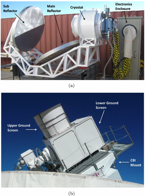
Figure 1. (a) The QUIET instrument before placement upon mount, showing the electronics enclosure, cryostat, and reflectors. (b) The mounted instrument shown within an absorbing ground screen.
Download figure:
Standard image High-resolution imageTable 1. Instrument Overview
| Band | Q | W |
|---|---|---|
| Frequency (GHz) | 43.1 | 94.5 |
| Bandwidth (GHz) | 7.6 | 10.7 |
| No. of polarization assemblies | 17 | 84 |
| No. of differential-temperature assemblies | 2 | 6 |
| FWHM angular resolution (arcmin) | 27.3 | 11.7 |
| Field of view (°) | 7.0 | 8.2 |
| ℓ range | ∼25–475 | ∼25–975 |
| Instrument sensitivity (μKs1/2) | 69 | 87 |
Download table as: ASCIITypeset image
We note that the QUIET receiver is unusual in that it is a polarimetry array, primarily sensitive to the polarization of the microwave sky rather than the total power from the sky. The calibration of QUIET (including measurement of beam properties and signal responsivities) therefore proceeds directly from the polarimetry data, rather than from unpolarized calibrators. The subset of QUIET differential-temperature assemblies provide ancillary data for assessing the atmospheric quality, improving the pointing model, and other systematic checks.
The following sections describe the observing site and strategy, optics, cryogenics and the optical window properties, polarimeter and differential-temperature assemblies, electronics, and calibration tools. Finally, we present a detailed description of the performance of both receivers.
2. OBSERVING SITE AND STRATEGY
Observations were performed at the Chajnantor plateau at 5080 m altitude in the Atacama Desert of Northern Chile (67°45'42''W 23°1'42''S). Atmospheric conditions were monitored using data from a 183 GHz line radiometer located at the APEX telescope (Güsten et al. 2006), ∼2.5 km away from the QUIET site. Typical atmospheric optical depths in our observing bands over all scanning elevations at Chajnantor are 0.02–0.1 (Figure 2). The median precipitable water vapor (PWV) was 1.2 mm (0.9 mm) during the Q-band (W-band) observing season. The data fraction surviving data selection for the Q-band (W-band) arrays are 82% (75%) of the data below the median PWV, and 59% (54%) of the data above the median PWV. The Q-band atmospheric absorption lines are dominated by oxygen, while the W-band has additional contamination from water vapor, so poor weather conditions will have a greater effect on the W-band data quality.
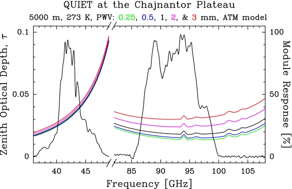
Figure 2. Zenith optical depth for typical atmospheric conditions at the Chajnantor plateau (left scale) and representative QUIET module bandpass responses (right scale). The atmospheric spectrum is calculated with the ATM model from Pardo et al. (2001).
Download figure:
Standard image High-resolution imageWe employed a fixed-elevation, azimuth-scanning technique: a ∼15° × 15° field (the fields are given in Table 2) was scanned in azimuth as it drifted through the ∼7° (∼8°) field of view for the Q-band (W-band) array. These constant elevation scans (CES) typically lasted ∼40–90 minutes. The telescope then re-tracked the field center and began another CES. By scanning at constant elevation for a given scan, we observed through a constant column density of atmosphere so that only weather variations within a scan contributed an atmospheric signal. Most calibration sources were observed at constant elevation, but occasionally we employed raster scans, changing elevation between azimuth slews to more rapidly observe a calibration source.
Table 2. Summary of Observations
| Band | Q | W | |
|---|---|---|---|
| Season start | 2008 Oct 24 | 2009 Aug 12 | |
| Season end | 2009 Jun 13 | 2010 Dec 22 | |
| Total observing hours | 3458 | 7426 | |
| CMB observing (%) | 77 | 72 | |
| Galactic observing (%) | 12 | 14 | |
| Calibration (%) | 7 | 13 | |
| Other (%) | 4 | 1 | |
| CMB Fields | J2000 Center (R.A., Decl.) | Q (hours) | W (hours) |
| CMB-1 | 12h04m −39° | 905 | 1855 |
| CMB-2 | 05h12m −39° | 703 | 1444 |
| CMB-3 | 00h48m −48° | 837 | 1389 |
| CMB-4 | 22h44m−36° | 223 | 650 |
Notes. The partition of the Q-band and W-band seasons by observation type (hours do not include data cuts obtained during data analysis for glitches, poor noise, etc.). "Other" includes data taken during engineering tests, aborted scans, etc.
Download table as: ASCIITypeset image
The infrastructure and three-axis driving mount previously used for the CBI experiment (Padin et al. 2002) was refurbished for QUIET, in part to enable rapid azimuth scanning. The mount control software is an augmented version of the CBI control system. The principal modifications included the addition of support for rapid scanning of the azimuth axis of the mount and for monitoring and archiving of data from the QUIET receiver. This software consists of a central control and data collection program, a graphical user interface program, a real-time computer running the VxWorks31 operating system to control the telescope mount, and a real-time computer running Linux to control the receiver. The mount was operated by a queue of non-interactive observing scripts written in a custom control language. The modifications supported high scanning accelerations without overwhelming the countertorque in the anti-backlash system of the azimuth drive. Tracking accuracy is therefore sacrificed for high scanning speeds and accelerations. However, accurate pointing information can be reconstructed during the data analysis from frequent readouts of the axis encoders and a dynamic model of the mechanical response of the mount. To facilitate this, the CBI control system was also modified to acquire encoder readouts at 100 Hz. The modified control system supports scans with coasting speeds of up to 6° s−1 and turnaround accelerations of up to 1 5 s−2. The accuracy of the encoder readout time stamps is ∼0.5 ms. The worst-case following error (the difference between the commanded trajectory and the encoder-read trajectory) was ∼8' at maximum acceleration during azimuth turnarounds. Both the timing and the following errors resulted in negligible pointing errors during the observing seasons (pointing accuracy is discussed further in Section 8.6). We achieved a mean azimuthal scan speed of ∼5° s−1. As each 15° × 15° observing field rises, its azimuthal extent with respect to the fixed telescope mount increases. As a result, the telescope azimuth slew size increases for higher elevation scans. This results in an elevation dependent scanning speed on the sky of ∼2° s−1, and scan frequencies between 45 and 100 mHz. Avoiding scanning through the azimuth limit leads to an upper elevation limit; the mount azimuth limit is ∼440° (80° past one full rotation), forcing an upper elevation limit of 75° for CMB scans. The lower limit of the elevation range of the mount is 43°.
In addition to the azimuth and elevation axes, the mount provides a third rotation axis through the boresight. This boresight angle ("deck angle") was rotated once per week in order to separate the polarization on the sky from that induced by systematic errors such as leakage from temperature to polarization.
3. OPTICS
The optical chain consists of a classical side-fed Dragonian antenna (Dragone 1978) coupled to a platelet array of diffusion-bonded corrugated feed horns cooled to ≃20 K (≃27 K) inside the Q-band (W-band) cryostat. The outputs of these optical elements are directed into the polarimeter and differential-temperature assemblies described in Sections 5.1 and 5.3, respectively. The main reflector (MR) and sub-reflector (SR) as well as the aperture of the cryostat are enclosed by an ambient temperature (≃ 270 K), absorbing ground screen. The design and characterization of the telescope, feed horns and ground screen are described in Sections 3.1, 3.2, and 3.3, respectively. The optical performance, as measured by the main beam, the sidelobes and the instrumental polarization, is described in Sections 3.4, 3.5, and 3.6, respectively.
3.1. Telescope
The telescope design requirements include: a wide field of view, excellent polarization characteristics, minimal beam distortion, minimal instrumental polarization, minimal spillover, and low sidelobes that could otherwise generate spurious polarization. The latter requirements have often been met by CMB experiments by using either classical, dual offset Cassegrain antennas (e.g., Barkats et al. 2005), Gregorian antennas (e.g., Meinhold et al. 1993), or shaped reflectors (e.g., Page et al. 2003b). QUIET is the first CMB polarization experiment to take advantage of the wide field of view enabled by a classical Dragonian antenna (Imbriale et al. 2011). An additional advantage of the classical Dragonian antenna is that it satisfies the Mizuguchi condition (Mizugutch et al. 1976), which, when combined with the very low cross-polar characteristics of the conical corrugated feed horns, yields very low antenna contribution to the instrumental polarization. As pointed out by Chang & Prata (2004), a classical Dragonian antenna affords two natural geometries, a front-fed design and a side-fed (or crossed) design. QUIET uses the side-fed design because it allows for the use of a larger cryostat, and hence focal plane array, without obstructing the beam.
3.1.1. Telescope Design
The design of the reflectors follows the procedure outlined by Chang & Prata (2004) and is augmented with a physical optics program (Imbriale & Hodges 1991) to predict beam patterns. This procedure relies on the specification of the first five design parameters given in the top half of Table 3 and shown in Figure 3. Once these parameters are specified, a number of other useful parameters can be calculated including the MR focal length and the SR eccentricity, and these are listed in the lower half of Table 3. The actual MR circular diameter was decreased slightly to 1400 mm, as noted by the actual value in Table 3, in order to avoid beam blockage from the SR. Similarly, the actual SR circular diameter was increased slightly, also to 1400 mm, and this resulted in an increased value of the actual SR edge angle given by 20° in Table 3. The oversized SR reduces feed spillover for the horns on the edge of the array. The design values (not the actual values) shown in the top half of Table 3 were used to establish the calculated values shown in the lower half of Table 3.
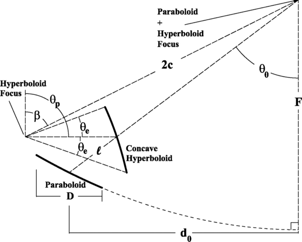
Figure 3. Scaled schematic of the QUIET side-fed Dragonian antenna shows a number of the useful design parameters. Table 3 provides a description of each parameter and its value.
Download figure:
Standard image High-resolution imageTable 3. Telescope Design Parameters
| Description, Parameter | Design/Actual Value |
|---|---|
| MR circular aperture diameter, D | 1470/1400 mm |
| SR edge ∠, θe | 17°/20° |
| MR-SR separation, ℓ | 1270 mm |
| MR offset ∠, θ0 | −53° |
| ∠ between MR and horn axes, θp | −90° |
| Calculated Value | |
| MR focal length, F | 4904.1 mm |
| SR eccentricity, e | 2.244 |
| ∠ between SR and MR axis, β | −6337 |
| SR interfocal distance, 2c | 6516.1 mm |
| MR offset distance, d0 | 4890.2 mm |
Notes. The design values in the top half of the table were used to establish the calculated values in the lower half of the table. For the first two parameters, the actual values listed supersede the design values for the purpose of fabrication. Negative angles are measured clockwise with respect to the vertical axis shown in Figure 3.
Download table as: ASCIITypeset image
3.1.2. Telescope Fabrication and Alignment
The telescope consists of two reflectors, the receiver cryostat (Figure 1(a)) and the structure that supports them (the "sled"). The reflectors are machined from solid pieces of aluminum 6061-T6, light-weighted on the reverse side, and attached with adjustable hexapod struts and turnbuckles to the sled. The sled in turn is mounted on a deck structure (Figure 1(b)), which also supports the ground screen, the receiver electronics enclosure, the telescope drive crates, the uninterruptible power supply, and the expanded steel walkways. The deck is attached directly to the deck bearing.
After the fabrication of the reflectors and sled, the telescope was assembled and pre-aligned using a MetricVision MV200 laser radar. This system was used to measure both the reflector surfaces as well as the absolute positions of tooling balls on the perimeter of each reflector once the reflectors were aligned to the focal plane. The rms deviations from the MR and SR design surfaces are 38 μm and 28 μm, respectively, once a small fraction (< 1%) of the outlier measurements from the perimeter of each reflector are removed.
A three-dimensional model of the telescope was constructed that included tooling balls mounted on the cryostat face with well measured displacements from the platelet array. Using the model, a transformation matrix was established that mapped turnbuckle adjustments to tooling ball displacements for each reflector (Monsalve 2012). This model was used to align the mirrors at the site as follows: after assembly at the site, the distances between the tooling balls were measured with a custom-built vernier caliper with a range of 2.4 m. The transformation matrix was inverted and translated into the adjustment required to the turnbuckles on the back of the mirror. The turnbuckles were adjusted and all parameters were re-measured. This method enabled convergence to an aligned state after just three iterations. The 17 measurements used to establish the position of the SR with respect to the cryostat (for both the Q- and W-band systems) yielded an rms error of <400 μm when compared to the ideal positioning. Similarly, the 14 measurements used to establish the position of the MR with respect to the SR yielded an rms error of <500 μm when compared to the ideal positioning as established using the laser radar. Tolerance studies allowing for comparable displacements show that this level of alignment error has minimal impact on the optical performance.
3.2. Feed Horns
The requirements for the feed horns include high beam symmetry, efficiency, gain, and bandwidth, as well as low sidelobes and cross-polarization. These requirements are satisfied by conical, corrugated feed horns (Kay 1962; Clarricoats & Olver 1984). Standard production techniques for corrugated feed horns (e.g., computer-numerically-controlled lathe machining and electroforming) are prohibitively costly for the large number of feeds for the W-band array. A lower-cost option is described in the next subsection.
3.2.1. Platelet Array Design
A 91-element W-band and a 19-element Q-band platelet array of hexagonally-packed, conical, corrugated feed horns were designed for QUIET (Gundersen & Wollack 2009; Imbriale et al. 2011). Each array is machined from aluminum 6061-T6 and consists of a number of thin platelets each with a single corrugation, a number of thick plates each with multiple corrugations, and a base plate. The assembly of platelets and plates is then diffusion bonded together. Table 4 provides the parameters of each array.
Table 4. Platelet Array Design Parameters
| Frequency | No. of | L × W × H | Mass | Aperture | Throat | No. of | Horn | Semi-flare |
|---|---|---|---|---|---|---|---|---|
| (band/GHz) | Feeds | (mm × mm × mm) | (kg) | Diameter | Diameter | Grooves | Separation | Angle |
| (mm) | (mm) | (mm) | (degrees) | |||||
| Q/39–47 | 19 | 281.7 × 427.3 × 370.1 | 43.7 | 71.78 | 6.69 | 104 | 76.20 | 76 |
| W/89–100 | 91 | 129.1 × 427.8 × 370.5 | 20.6 | 31.62 | 2.97 | 103 | 35.56 | 76 |
Download table as: ASCIITypeset image
Due to the side-fed geometry of the telescope, the feed horns must have relatively high gain (≃ 27 to 28 dB) in order to provide a low edge taper of ⩽ − 30 dB for both the Q- and W-band systems. This dictates the aperture size of the feed horns and hence the horn-to-horn spacing. For the W-band horns, this spacing is commensurate with the size of the modules. Most of the dimensions of the Q-band horns are scaled by the ratio of the frequencies (∼ 90/40 = 2.25), which results in a Q-band horn spacing that is larger than the Q-band modules. These horn spacings give rise to angular separations of 175 (082) between adjacent beams in the Q (W) systems and result in fields of view of 70 and 82 for the Q and W systems, respectively.
The number of corrugations is fixed at three per wavelength for each horn and a semi-flare angle of 76 is chosen using a design procedure that ensures both acceptable cross-polar levels and return loss (Hoppe 1987, 1988). This optimization procedure also adjusts the depth of the first six corrugations of each horn in order to reduce the predicted reflection coefficient to better than −32 dB over the full anticipated band of operation.
3.2.2. Platelet Array Testing
A vector network analyzer (VNA) was used to measure the return loss of each horn in each array. Each measurement consisted of attaching one horn in a platelet array to one port of the VNA using a commercially available circular-to-rectangular transition. A sheet of microwave absorber was placed at 45° in front of the horns at a distance of ≃ 1 m. The return losses for five of the 19 Q-band horns are shown in Figure 4 and are similar for the W-band feed horns. Maximum reflection strengths (negative return loss) are listed in Table 5. For comparison, individual electroformed horns that are identical in design to the Q- and W-band horns were fabricated. The array values in Table 5 are comparable to but not quite as good as the electroformed horns or the theoretical predictions, both of which were < − 30 dB across the band.
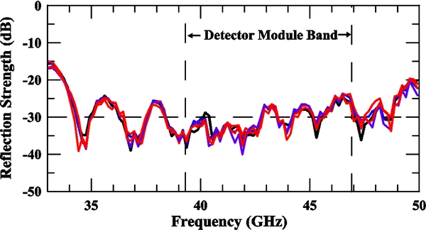
Figure 4. Return loss measurements for five of the 19 Q-band horns. None of the other 14 horns show a return loss greater than 1 dB above the measurements shown here.
Download figure:
Standard image High-resolution imageTable 5. Measured Platelet Array Performance
| Frequency | FWHM | Gain | Crosspol | Reflection | Insertion |
|---|---|---|---|---|---|
| (band/GHz) | (deg) | (dB) | E/H | Strength | Loss |
| (dB) | (dB) | (dB) | |||
| Q/39–47 | 8.3–6.9 | 27.2–28.5 | < − 34/ − 29 | < − 25 | < − 0.1 |
| W/89–100 | 8.3–7.4 | 27.1–28.0 | < − 31/ − 29 | < − 24 | < − 0.1 |
Download table as: ASCIITypeset image
Beam patterns were measured for all 91 horns in the W-band array and 13 out of 19 horns in the Q-band array. A synthesizer combined with × 3 and × 6 multipliers generated the source signals at 40 and 90 GHz, respectively. A standard gain horn was used as a source antenna. The platelet arrays were mounted on an azimuth-elevation mount so that the source was in the far-field of the platelet array horns. The source signals were modulated at 1 kHz and a lock-in amplifier connected to a detector diode on the platelet array detected the signal. A co-aligned alignment laser ensured that the source horn and platelet array horn were parallel and axially aligned to each other. A digital protractor with an accuracy of ±005 ensured that the source and receiver horn's polarization axes were coincident for the copolar patterns or perpendicular to each other for the cross-polar patterns. Several measurements were made on each horn including E- and H-plane copolar patterns as well as their corresponding cross-polar patterns. The patterns were taken by keeping the source horn static and rotating the platelet array horn in azimuth about a vertical axis that intersected the horns phase center. A detailed description of this procedure is given in Clarricoats & Olver (1984).
The beam patterns of typical Q-band and W-band horns are shown in Figure 5. This figure shows both E- and H-plane copolar patterns as well as cross-polar patterns for the platelet feeds and for an electroformed feed with identical design parameters. The figure also shows the theoretical model responses. In all cases the E- and H-plane copolar patterns are consistent with both the model and the electroformed feed measurements out to the −30 dB level. Upper limits of −34 (−31) dB are set on the E-plane cross-polar levels for Q-band (W-band). The H-plane cross-polar patterns are not in as good agreement with the model, which predicts both E- and H-plane cross-polar levels at the < − 40 dB level. The largest discrepancies are similar in shape to the Q-band H-plane cross-polar measurements shown in Figure 5 and have a non-null cross-polar boresight response. This type of response is typical of angular misalignment between the source and receiver probes, and the level of the response is consistent with the precision of the digital level. The W-band H-plane cross-polar response does have a null on boresight and is likely the true cross-polar response. The fact that the cross-polar responses of the individual feed horns in the platelet array are consistently higher than the corresponding electroformed horns' responses suggests that either the machining or the diffusion bonding process leads to somewhat compromised performance. However, none of the measured feeds has cross-polar levels > − 29 dB. Table 5 summarizes the results of the beam pattern measurements.

Figure 5. Beam pattern measurements of a typical Q-band (top) and W-band (bottom) horn in each platelet array along with an electroformed equivalent horn are shown. The left subfigures show the E-plane results and the right subfigures show the H-plane results. The solid line in each case shows the theoretical prediction of the copolar responses. The theoretical predictions of the cross-polar responses are all below −40 dB and are not shown. The H-plane cross-polar responses are measured at the −30 to −33 dB level for both Q- and W-band platelet array horns as well as for their electroformed equivalents.
Download figure:
Standard image High-resolution imageUpper limits on the insertion loss were obtained during the return loss measurements of both the W-band and Q-band platelet arrays by placing a flat aluminum plate in front of the horn and generating an effective short. In both cases the measured reflection strength allows a lower bound to be set on the feeds' room temperature transmission efficiency of >99%. Assuming solely ohmic losses, this transmission efficiency is expected to increase to >99.5% upon cooling to 25 K as the electrical resistivity of the horns decreases with temperature (Clark et al. 1970).
3.3. Ground Screen
An absorbing, comoving ground screen is employed to shield the instrument from varying ground and Sun pick-up and provide a stable, essentially unpolarized emission source that does not vary during a telescope scan. The ground screen structure (Figure 1(b)) consists of two parts: the lower ground screen is an aluminum box that encloses both reflectors and the front half of the cryostat; the upper ground screen (UGS) is a cylindrical tube that attaches to the lower ground screen directly above the MR. The external surface of the ground screen is coated in white paint in order to reduce diurnal temperature variations and to minimize radiative loading. Following the approach used by the BICEP experiment (Takahashi et al. 2010), the interior of the ground screen is coated with a broadband absorber32 that absorbs radiation and re-emits it at a constant temperature, allowing the ground screen to function as an approximately constant Rayleigh–Jeans source in both Q- and W-bands. The UGS was installed in 2010 January (a third of the way through the W-band season), and it was particularly useful in eliminating spillover past the SR, as shown in Sections 3.5.2 and 3.5.3.
3.4. Main Beam Performance
The main beam profiles are primarily determined from observations of Jupiter. Additional observations of Taurus A (hereafter Tau A) are performed to check the main lobe response, to measure the polarized responsivity, to determine the polarization angles, and to characterize instrumental polarization. Tau A and Jupiter are used for main beam characterization since they are, respectively, the brightest polarized and unpolarized, compact sources in the sky. Figure 6 shows beam patterns of Jupiter for a differential-temperature assembly in each of the Q- and W-band arrays. These measurements are consistent with the lower signal-to-noise main beam profiles measured using Tau A once the slightly different instrumental bandpasses, source spectra, and positions in the focal plane are taken into account. The main beam is used to compute the main beam solid angle ΩB, the main beam forward gain, Gm = 4π/ΩB, and the telescope sensitivity,
in terms of the effective frequency,
for a given instrumental bandpass f(ν) and source spectrum σ(ν). Equations (1) and (2) explicitly assume Gm∝ν2. The source spectra of Tau A and Jupiter are based on the Wilkinson Microwave Anisotropy Probe (WMAP) measurements (Weiland et al. 2011). A Tau A source spectrum with σ∝ν−0.302 is assumed for the calculation of the effective frequency for the Tau A measurements. An empirical fit to WMAP's measurements of Jupiter's brightness temperatures yields a source spectrum of the form
Similarly a source spectrum of the form

is used to compute the effective frequency for unresolved CMB fluctuations, where x = hν/kBTCMB.
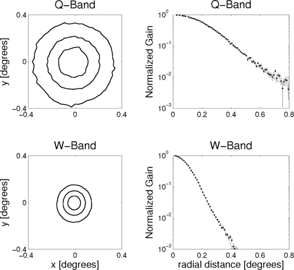
Figure 6. Normalized beam maps of Jupiter are shown on the left for representative differential-temperature assemblies for the Q- and W-band systems with contours at 20%, 50%, and 80% of the peak power. The corresponding azimuthally-averaged beam profiles for each map are shown on the right in comparison with the theoretical prediction (solid line). Similar maps and profiles of Tau A were measured using the polarimeter assemblies but at a reduced signal-to-noise.
Download figure:
Standard image High-resolution imageTable 6 provides a summary of the mean values of these quantities for the Q-band and W-band polarization and differential-temperature modules for a source spectrum of the form given in Equation (4). The Q-band total power values are for the lone Q-band differential-temperature assembly, while the Q-band polarization values are for the central pixel, which is typical for the array. Both the W-band total power and polarization values shown in Table 6 are averaged over the respective differential-temperature and polarization array elements using an inverse-variance weighting.
Table 6. Main Beam Performance Parameters
| νe | FWHM | ΩB | Gm | Γ | |
|---|---|---|---|---|---|
| (GHz) | (deg) | (μsr) | (dBi) | (μK Jy−1) | |
| QP | 43.0 | 0.455 | 74.3 | 52.3 | 237 |
| QT | 43.4 | 0.456 | 78.0 | 52.1 | 222 |
| WP | 94.4 | 0.195 | 13.6 | 59.6 | 269 |
| WT | 95.7 | 0.204 | 15.6 | 59.1 | 228 |
Notes. Mean effective frequencies, FWHM beam sizes, main beam solid angles, main beam forward gains, and telescope sensitivities for both the polarization (subscript P) and differential-temperature (subscript T) assemblies assuming a CMB-like, broadband source with a spectrum given by Equation (4).
Download table as: ASCIITypeset image
The shape of the main beam and its uncertainties are used to compute the instrumental window function and its associated uncertainties (Monsalve 2010). Initially, an arbitrarily oriented, two-dimensional, elliptical Gaussian beam is fit to the data shown in Figure 6. If σa and σb represent the beam widths of the semi-major and semi-minor axes of the elliptical Gaussian (with σa ⩾ σb), then the elongation is defined by  = (σa − σb)/(σa + σb). Typical elongations were found to be <0.02 and averaged about 0.01. This low elongation, and the fact that the CMB scans use a combination of natural sky rotation and deck angle rotation, imply that the beams are well described by an axially-symmetric beam. The symmetrized beam is expressed as a one-dimensional Hermite expansion (Monsalve 2010), and this expansion is used to compute the beam transfer function and its covariance matrix (Page et al. 2003a).
3.5. Sidelobe Characterization
Two different methods are used to measure sidelobes. These included pre-deployment antenna range measurements and in situ measurements of a bright, near-field source. In addition, unintentional measurements of the Sun in the sidelobes also enabled their characterization. These three measurements and their results are discussed in more detail here.
3.5.1. Antenna Range Measurements of Sidelobes
The telescope was installed on the Jet Propulsion Laboratory's Mesa Antenna Measurement Facility for measurements of both the main lobe and far sidelobes at both 40 and 90 GHz. The telescope was mounted on an elevation-over-azimuth positioner with 4'' pointing accuracy. Individual electroformed versions of the Q- and W-band horns, described in Section 3.2.2, were used for the range measurements. The range measurements were conducted before the ground screens were fabricated, so the sidelobe results are only appropriate for the telescope in its bare configuration. The measurements made use of the facility's Scientific Atlanta model 1797 heterodyne receiver system, which enabled repeatable measurements down to −90 dB of the peak power level. A combination of a source synthesizer, multiplier and amplifier was used to generate ≃ 100–200 mW of power at each frequency. The sources were separately connected to corrugated feeds at the focus of a small Cassegrain antenna at a distance of 914 m from the telescope. Due to limitations of the mount, only a simple principal plane cut within ±90° of the telescope boresight (in the plane shown in Figure 3) was performed for a number of arrangements of the source/receiver antennas. These arrangements included moving the receiver horn to a few positions in the focal plane and rotating the source and receiver horns for both E- and H-plane cuts.
The results for one feed horn position for each of the Q- and W-band arrays are shown in Figure 7. In each case the feed horn position that was tested corresponds to the top row of the respective platelet array, furthest from the MR and directly above the central feed horn. Cross-polar measurements were not made on the antenna range since they are made during routine calibrations. The main lobe beam sizes compare well with initial theoretical predictions (Imbriale et al. 2011); however, the near-in (i.e., within ±5° of the main lobe) sidelobe levels do not. It is also shown in that paper that the predicted envelope of near-in sidelobes matches well with the observations once the measured reflector surface imperfections are included. The surface imperfections caused the near-in sidelobe levels to increase by as much as 15 dB in some regions.
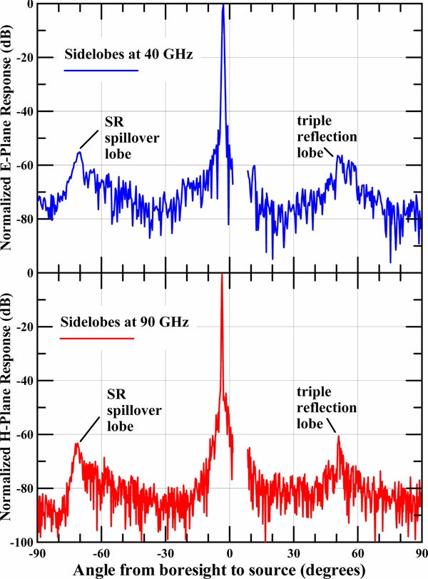
Figure 7. Results from the antenna range measurements with no ground screens in place. The top measurements are the 40 GHz E-plane results for a horn located in the top row, 20.46 mm above the central horn. The bottom measurements are the 90 GHz H-plane results for a horn located in the top row, 23.87 mm above the central horn. The gap in the measurements from boresight angles of +15 to +85 is due to mount-related elevation angle limitations. The two most prominent far sidelobes are the triple reflection sidelobe and the SR spillover lobe as indicated in each figure. The optical paths associated with these lobes are shown in Figure 9. Top row horns, such as these, are most susceptible to each of these lobes due to their location in the focal plane.
Download figure:
Standard image High-resolution imageThe two dominant far sidelobes are the SR spillover lobe and the "triple reflection" lobe, both predicted in Imbriale et al. (2011). The SR spillover lobe is broad, arises from direct coupling into the feed horn, and is located ∼70° from boresight. The triple reflection lobe is due to an additional reflection off the SR (as indicated in Figure 9) and it is located ≃ 50° from boresight in the opposite direction from the SR spillover lobe. The amplitudes of each lobe for the W-band case are −60 to −62 dB, while they are −58 to −59 dB for the Q-band measurement. These amplitudes are both 5–7 dB above the uncorrected predictions of Imbriale et al. (2011).
3.5.2. Source Measurements of Sidelobes
The performance of the UGS was assessed using the W-band array in 2010 January. For these measurements, a polarized, modulated 92 GHz oscillator was placed in the near field of the telescope at a distance of approximately 15 m. The telescope was scanned over its entire azimuth and elevation range at four different deck angles (0°, 90°, −90°, −180°). The top and middle panels in Figure 8 show measurements before and after the installation of the UGS, respectively. The main sidelobe feature at the bottom of the top map corresponds to the line of sight over the SR. This feature is clearly removed by the UGS. The remaining sidelobes were caused by holes in the floor of the lower ground screen below the SR. A third measurement taken after placing an absorber over these holes (bottom panel in Figure 8) verifies this and displays the sidelobe performance in the final ground screen configuration. The UGS was not in place during any of the Q-band observing season nor during the first third of the W-band observing season.
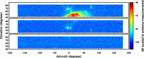
Figure 8. Sidelobe measurements for a W-band module located on the edge of the array, with the deck angle set at −180° and the near-field source located at an azimuth of ≃20° and an elevation of ≃ − 5°. (Top) Measurements with only the lower ground screen. The lobe seen at the bottom of the map is from spillover past the SR. This lobe is removed after the installation of the UGS. (Middle) Measurements with the lower ground screen and UGS installed. The lobe at the top is due to holes in the absorber from the ground screen structure, and is present before the UGS was added as well, but its position has shifted slightly because the source was moved between measurements. (Bottom) Results with the complete ground screen installed and with an additional absorber placed over holes in the floor of the lower ground screen. The color scale is the same between all three measurements and has been normalized to match the antenna range measurements. The UGS reduces the far sidelobes by at least an additional 20 dB below the levels shown in Figure 7.
Download figure:
Standard image High-resolution image3.5.3. Sun Measurements of Sidelobes
Before the installation of the UGS, the Sun was occasionally detected in the sidelobes. This is particularly apparent once the data are binned into maps in "telescope boresight-centered" coordinates (Chinone 2011). The Cartesian basis of this coordinate system has  oriented along the feed horn boresight,
  oriented along the telescope boresight, and
  . If
. If  is directed toward the Sun, the corresponding spherical coordinates of the Sun are defined to be
  , and
, and  . In these coordinates, the telescope would be pointed directly at the Sun at θ = 0, but it never is (intentionally) pointed closer than ∼30°. These Sun-centered sidelobe maps are shown in Figure 9 for a top-row module (as the SR spillover is dependent on focal plane position, and the top row has the strongest coupling). Figure 9(a) shows the optical path of these sidelobes before the installation of the UGS for a Q-band horn, and Figures 9(c) and (d) show measurements of the far sidelobes for the W-band system before and after installation of the UGS, respectively. Figure 9(d) confirms that both far sidelobes are eliminated by the UGS. The ϕ = 0° − 180° horizontal line in Figure 9 corresponds to the principal plane measurement shown in Figure 7, and both show the SR spillover lobe and triple reflection lobe before the installation of the UGS. The amplitudes of the two far sidelobes measured with the Sun are consistent with the ∼ − 60 dB levels obtained with the range measurements shown in Figure 7. Data with the Moon or Sun in the sidelobes were excised in the Q-band analysis (QUIET Collaboration et al. 2011) as well as during the first third of the W-band season (QUIET Collaboration et al. 2012). The addition of the UGS for the W-band data, in combination with azimuth filtering and data rejection used for the Q-band data, makes the spurious polarization signal due to sidelobes a negligible effect on the B-mode measurements.

Figure 9. Sidelobe characterization using the Sun. (a) The optical paths that give rise to the triple reflection and spillover sidelobes are shown before the installation of the UGS. (b) The telescope boresight-centered map of the Sun (see the text) is shown before the installation of the UGS for a Q-band feed horn in the top row, nearest to the vertical centerline. The sharp spike induced by the triple reflection is seen at (θ, ϕ) ≃ (50°, 180°), while the large area of sidelobe contamination just under the ϕ = 0° line is induced by the SR spillover. (c) The telescope boresight-centered map of the Sun is shown for a horn in a similar position in the W-band array before the UGS installation. (d) The same map is shown for the same W-band horn after the UGS installation and after the holes in the lower ground screen floor were filled with absorber.
Download figure:
Standard image High-resolution image3.6. Leakage Beams
The leakage beams quantify both the Q and U detector diodes'33 responses to an unpolarized source, as well as the leakage that can convert a sky Q into a measured U or a sky U into a measured Q. In order to assess these various forms of leakage, daily observations of Jupiter and/or Tau A were performed. These produce beam maps that are subsequently decomposed into their respective beam Mueller fields following O'Dea et al. (2007). The beam Mueller fields are related to the copolar and cross-polar components of the dual, orthogonal polarizations supported by the feed system. For a linearly polarized source with Stokes parameters Isrc, Qsrc, Usrc (assuming Vsrc = 0), degree of linear polarization  , and position angle γPA = (1/2)tan −1(− Usrc/Qsrc), the output voltage dQ of a Q diode as a function of instrumental flux density gain gQ and instrumental position angle ψ is given by

where mQI and mQU are the Mueller fields representing the I-to-Q and U-to-Q leakage beams, mQQ is the extracted Q polarization beam and τ is the opacity with typical values given in Figure 2. Similarly, the output voltage of a U diode is given by

where mUI and mUQ are the corresponding leakage beams, and mUU is the U polarization beam. In each of these expressions, the factor g is the product of the receiver responsivity (described in Section 8.4) and the telescope sensitivity Γ given by Equation (1). The instrumental position angle is given by ψ = η + ϕd where η is the parallactic angle of the beam center and ϕd is the deck angle.34 For a number of sources the parallactic angle coverage is not very large, so beam maps at various deck angles are necessary in order to vary the outputs of the Q and U detector diodes. This is particularly true for Tau A, which (due to the mount's lower elevation limit) is only tracked over a limited azimuth range, and this translates into a limited range of parallactic angles. Figure 10 shows the results of this extraction of the leakage and polarized beams for a Q and U diode pair behind the central W-band horn. A similar figure is shown in Monsalve (2010) for the Q-band system.
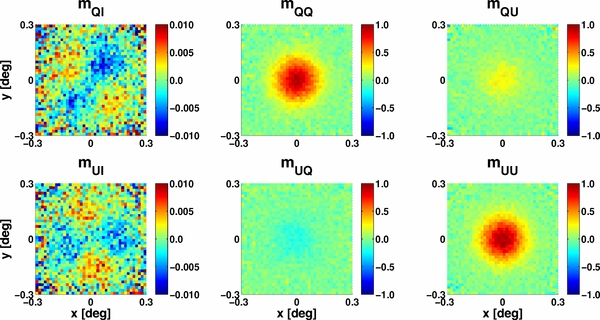
Figure 10. Extracted Mueller fields are shown for a Q and U diode pair behind the central horn of the W-band array. For the purpose of this figure, the mQQ and mUU fields have been normalized to one and the normalizations have been applied to the off-diagonal fields. A ≃ 0.4% quadrupole term is evident in the mQI and mUI leakage beams, while no higher order structure is evident in the mQU or mUQ leakage beams at the ≃ 0.1% level. As described in Section 3.6, the monopole contribution to the mQU and mUQ leakage beams can be absorbed into the detector angle, which is measured during the calibration procedure. Similar results for the Q-band central pixel are given in Monsalve (2010).
Download figure:
Standard image High-resolution imageThe mQI and mUI Mueller fields are of particular importance since they characterize the instrumental polarization. Instrumental polarization can be generated by any of the elements in the optical path including the reflectors, the curved cryostat window, the IR blocker, the feed horns, the septum polarizers and the modules themselves. In Appendices A and B, specific expressions are derived for these leakage terms for the modules and the septum polarizers. These two elements are the primary cause of the monopole leakage contribution to the mQI and mUI Mueller fields. The median W-band monopole leakage is 0.25% and is lower than the median Q-band monopole leakage. These Q- and W-band leakages measured with Jupiter and Tau A are consistent with those obtained from sky-dip measurements that are described in Section 8.4. As reported in QUIET Collaboration et al. (2011), the Q-band monopole leakage is the largest systematic error in the B-mode measurement at ℓ ∼ 100 where it begins to dominate the constraint on r at levels of r < 0.1. A naïve estimate of the impact of this leakage would cause it to dominate at a much higher level; however, a combination of sky rotation and frequent boresight rotation suppresses this systematic by some two orders of magnitude. The origins of the Q-band monopole leakage are described in more detail in Section 5.1.
The monopole leakage refers to the s00 term in the two-dimensional Hermite expansion of these leakage beams given by bleak(x, y) (Monsalve 2010). Here and in Figure 10 the coordinates (x = sin θsin ϕ, y = sin θcos ϕ) are telescope boresight-centered coordinates defined in Section 3.5.3. The leakage beams can be expressed as
where sij are the fit coefficients and the normalized basis functions fij(x, y) are
where σ is the Gaussian width of the symmetrized beam described in Section 3.4 and the Hi and Hj are Hermite polynomials.
Higher-order leakage terms, including dipole (s01 or s10) and quadrupole leakages (s11 or (s20 − s02)/2), can also arise due to the off-axis nature of the telescope and the imperfectly matched E- and H-plane feed horn patterns. The full array drift scans of Jupiter are particularly useful in measuring these quantities for every diode in the W-band array. Histograms of the peak amplitudes complete to i = j = 2 are shown in Figure 11 for the W-band array (similar results are provided for the central pixel of the Q-band array in Monsalve 2010). Additional terms in the expansion are also included, but they are consistently less than 0.1%. Leakages above 1% are quite rare and typical values are in the 0.2%–0.4% range. The W-band dipole and quadrupole leakages are typically slightly higher than those in Q-band. The systematic effects that these leakage beams generate for power spectrum estimation are provided for the Q-band results (QUIET Collaboration et al. 2011) and in the W-band analysis (QUIET Collaboration et al. 2012).
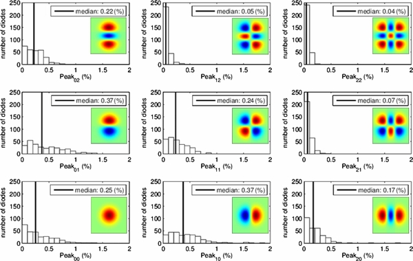
Figure 11. Histograms show the number of W-band diodes that have a maximum absolute value of the product |sijfij| (denoted Peakij on the ordinate) in a given percentile range for both the mQI and mUI leakage beams. The Hermite expansion term is also shown in each panel. A median value of all detector diodes is provided in each histogram and indicated with a vertical line. Similar results for the central pixel of the Q-band system are given in Monsalve (2010).
Download figure:
Standard image High-resolution imageThe mUQ and mQU Mueller fields measure the leakage of the incident Q Stokes parameter into the measured U Stokes parameter or the incident U Stokes parameter into the measured Q Stokes parameter. Curved reflector surfaces, imperfections in the septum polarizer, and imperfections in the phase switch are potential sources of this leakage. These primarily give rise to monopole leakage and effectively rotate the instrumental position angle. In the case that the ratios mQU/mQQ and mUQ/mUU are constant over the extent of the beam, the mUQ and mQU Mueller fields can be absorbed into the expressions for the two diode outputs with the definition of detector angles ψQ and ψU. The detector angles are defined by replacing the last two terms in each of Equations (5) and (6) with a single term as follows:
and
respectively. A Hermite decomposition of the mQU and mUQ Mueller fields shown in Figure 10 shows that they are simply related by a multiplicative factor to the mQQ and mUU fields. Thus they can be represented in terms of single-valued detector angles, ψQ and ψU and are not a source of systematic error. In order to achieve the maximum benefit of simultaneous Q/U detection, it is an important feature that the detector angles are separated by nearly integer multiples of 45° for each of the four diodes in a given module. This is the case for both the Q-band and W-band instruments (and the W-band instrument detector angles are shown in Section 8.5).
4. CRYOSTATS
4.1. Cryostat Design
The Q-band and W-band receiver arrays each has a dedicated cryostat (Figure 12). In each cryostat, cryogenic temperatures are achieved with two Gifford-McMahon dual-stage refrigerators. The first stage of the refrigerators provide cooling power to a radiation shield, maintained at ∼50 K (∼80 K) for the Q-band (W-band) cryostat. The difference in shield temperature between the W-band and Q-band instruments was not anticipated from the cryostat design, but ultimately did not greatly impact the module temperatures. Infrared radiation is reduced with 10 cm thick, 3 lb density polystyrene foam (Table 7) attached to the top of the radiation shield. The first stages of the refrigerators also provide a thermal break for the electrical cables. The second stages of the refrigerators provide cooling power for the feed horn array and the modules. The two stages are thermally isolated by G-10 rings.
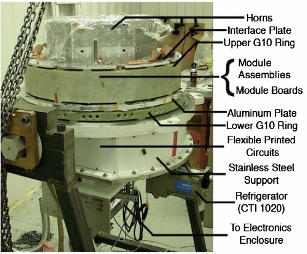
Figure 12. W-band cryostat with the vacuum shell and radiation shields removed.
Download figure:
Standard image High-resolution imageTable 7. Cryostat Optical Material Parameters
| Material | Index of | Thickness (mm) | Vendor | |
|---|---|---|---|---|
| Refraction | Q Band | W Band | ||
| UHMW-PE | 1.52 | 9.52 | 6.35 | McMaster-Carr |
| LD-PE | 1.52 | 0.127 | 0.127 | McMaster-Carr |
| Teflon | 1.2 | 1.59 | 0.54 | Inertech |
| Polystyrene foam | ⋅⋅⋅ | 101.6 | 101.6 | Clark Foam |
Note. Values for the index of refraction for teflon and UHMW-PE come from the best-fit values to VNA measurements at 90 GHz.
Download table as: ASCIITypeset image
4.2. Cryostat Performance
The cryogenic performance of the Q-band array is consistent with the design goals of (1) 20 K module temperatures and (2) that the module temperatures remain constant during a CES (CESes are described in Section 2) to within ±0.1 K. A temperature sensor located on an edge module in the Q-band cryostat had a mean temperature of 20.0 K with a standard deviation of 0.3 K throughout the season and a deviation of 0.02 K within a CES.
For the W-band array, additional heat loads from the active components and conduction through cabling from a factor of five more modules contribute to slightly higher module temperatures compared with the Q-band array. Taking this into consideration, the W-band modules were still warmer than expected by ∼3 K, likely as a result of both higher shield temperatures and a minor vacuum leak. A temperature sensor placed directly on the central polarimeter of the W-band array had a mean temperature of 27.4 K with a standard deviation of 1.0 K throughout the season, and a mean variation within a CES of 0.12 K. For each receiver array, both the variation of the module temperatures within a CES and throughout the season had a negligible impact on the responsivity (QUIET Collaboration et al. 2011, 2012).
4.3. The Cryostat Window
The vacuum windows for the Q-band and W-band cryostats are each ∼56 cm in diameter, the largest vacuum window to date for any CMB experiment. The vacuum windows must be strong enough to withstand atmospheric pressure while maximizing transmission of signal and minimizing instrumental polarization.
Ultra-high molecular weight polyethylene (UHMW-PE) was chosen as the window material after stress-testing a variety of window materials and thicknesses. The index of refraction was expected to be 1.52 (Lamb 1996). To make a well-matched anti-reflection coating for the UHMW-PE in the QUIET frequency bands, the window was coated with expanded teflon, which has an index of refraction of 1.2 (Benford et al. 2003). The teflon was adhered to the UHMW-PE window by placing an intermediate layer of low-density polyethylene (LD-PE) between the teflon and the UHMW-PE. The plastics were heated above the melting point of LD-PE while applying pressure with a clamping apparatus in a vacuum chamber to avoid trapping air bubbles between the material layers (the window material properties are included in Table 7). The band-averaged transmission was expected to improve from 90% to 99% for the Q-band array and from 91% to 98% for the W-band array by adding this anti-reflection coating to the windows.
An anti-reflection coated sample for the W-band window was measured using a VNA. The envelope of the transmission and reflection response were fitted to obtain values for the optical properties and material thicknesses (shown in Table 7, they matched literature values). The expected contributions to the system noise from loss were computed using published loss tangent values (Lamb 1996): ∼3 K (∼4 K) for the Q-band (W-band) windows. These values were confirmed within ∼1 K by placing a second window over the main receiver window and measuring the change in instrument noise.
The curvature of the window under vacuum pressure could introduce cross-polarization. A physical optics analysis of the W-band window was performed with the General Reflector Antenna Analysis (GRASP)35 package to investigate the effect of the curved surface on the transmission properties of the window. For these simulations we use a window curvature determined from measurements of the deflection of the window under vacuum, ∼7.5 cm. With a curved window, the central feed horn has negligible instrumental polarization. The edge pixel has 0.16% additional cross-polarization, where this is defined as leakage from one linear polarization state into the other linear polarization state. This −28 dB cross-polarization is of the same order as expected cross-polarization from the horns alone and would contribute indirectly to the cross-polarization coefficients mQU and mUQ given in Section 3.6.
5. QUIET POLARIMETER AND DIFFERENTIAL-TEMPERATURE ASSEMBLIES
QUIET uses HEMT-based low-noise amplifiers ("LNAs") with phase sensitive techniques, following the tradition of recent polarization-sensitive experiments such as DASI (Leitch et al. 2002), CBI (Padin et al. 2002), WMAP (Jarosik et al. 2003a), COMPASS (Farese et al. 2004), and PIQUE and CAPMAP (Barkats et al. 2005). Unlike those other experiments, however, QUIET uses a miniaturized design (Lawrence et al. 2004) suitable for large arrays. This design was realized in the QUIET module, a highly integrated package that replaced many waveguide-block components with microstrip-coupled monolithic microwave integrated circuit (MMIC) devices containing HEMTs. The modules have a footprint of 3.18 cm × 2.90 cm (W-band) and 5.08 cm × 5.08 cm (Q-band). Figure 13 shows the W-band array assemblies.

Figure 13. W-band array polarimeter and differential-temperature assemblies. The latter are shown on the right-hand side, yet to be installed.
Download figure:
Standard image High-resolution imageThe 17 Q-band and 84 W-band polarization assemblies and QUIET modules are described in Sections 5.1 and 5.2. The remaining two Q-band and six W-band modules are designed to measure the CMB temperature anisotropy ("differential-temperature assemblies") and are described in Section 5.3.
5.1. Polarimeter Assemblies
Each QUIET polarimeter assembly consists of (1) a septum polarizer, (2) a waveguide spreader, and (3) a module containing the integrated package of HEMT-based MMIC devices (Figure 14). The septum polarizer consists of a short circular-to-square transition into a square waveguide containing a septum (a thin aluminum piece with a stepped profile) in the center, which adds a phase lag to one of the propagating modes (Bornemann & Labay 1995). Given an incident electric field with linear orthogonal components Ex and Ey, where the x and y axis orientations are defined by the septum, the septum polarizer assembly sends a left-circularly polarized component  to one output port, and a right-circularly polarized component
  to the other output port. Thus the septum's spatial orientation is used to define the instrumental position angle. The output ports of the septum polarizer are attached to a waveguide spreader, which transitions from the narrow waveguide spacing of the septum-polarizer component to the wider waveguide separation of the module waveguide inputs. A more thorough mathematical description of the septum polarizer is given in Appendix B.1.
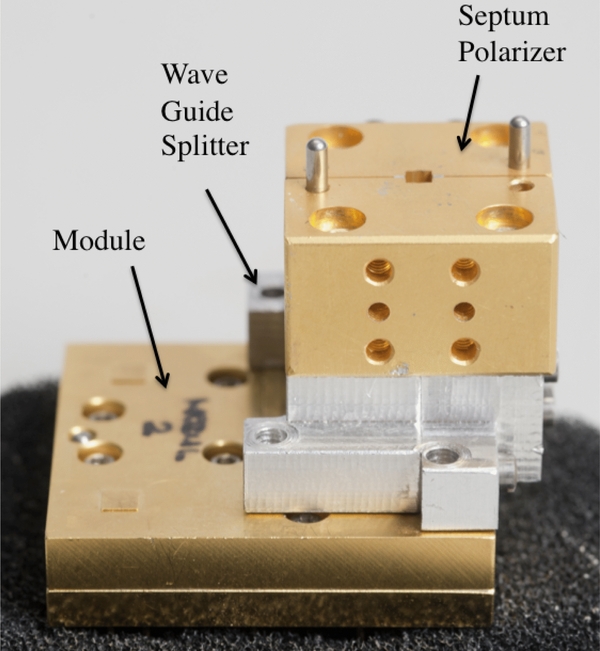
Figure 14. W-band polarimeter assembly. The module is more compact than previous generation correlators by an order of magnitude.
Download figure:
Standard image High-resolution imageThe scattering matrices, gains, and the temperature-to-polarization (monopole) leakage terms of both the Q-band and W-band septum polarizers are derived from VNA measurements. The scattering matrix and derived quantities for these terms are presented in Appendix B.1. Spectrum analyzer measurements of the Q-band modules in the laboratory show a degradation in the return loss near the low frequency end of the module's bandpass. When this return loss power is reflected off the septum polarizer and back into the module, it is amplified in the LNAs in the module legs and sent back out of the module to reflect again. This sets up an oscillation that renders the module incapable of measuring input signals. Therefore, a bandpass mismatch between the septum polarizer and module was deliberately introduced to send this return loss to the sky and prevent oscillations in the module output. The bandpass mismatch leads to an enhancement in the differential loss between the Ex and Ey transmissions at 47 GHz, causing a temperature-to-Stokes Q leakage of ∼1%, averaged over the module's bandpass. This estimate is consistent with leakage values derived from Tau A measurements (Section 3.6). W-band VNA measurements show no return loss degradation (measurements indicate −30 dB return loss, compared with −19 dB for the Q-band septum polarizers), and therefore no bandpass adjustments are needed. The VNA measurements predict a smaller leakage of ∼0.3%, so that it is subdominant to leakage due to optics. These measurements are consistent with monopole leakage values obtained from on-sky calibrators (see Section 3.6 and Figure 11). Note that since the optics leakage has a random direction relative to the polarimeter assembly leakage, the combined leakage averages to a smaller value and is randomly distributed both in sign and amplitude among modules. The isolation between the left- and right-circularly polarized ports was measured to be −22 dB for the Q-band septum polarizers, and −28 dB for the W-band septum polarizers.
5.2. Modules
The QUIET modules are used in the polarimeter and differential-temperature assemblies, functioning as pseudo-correlation receivers so that the output is a product (rather than sum or difference) of gain terms. The modules employ a high speed switching technique to reduce 1/f noise, and are an improvement on classical Dicke-switched radiometers (Dicke 1946) in that we switch between two sky signals, yielding an improvement of  in sensitivity (Mennella et al. 2003).
In a polarimeter assembly, the module receives as inputs the left (L) and right (R) circularly polarized components of the incident radiation, and measures the Stokes parameters Q, U and I, defined as
where the * denotes complex conjugation and we expect V to be zero but do not measure it.
Figure 15(a) shows a schematic of the QUIET module, in which L and R traverse separate amplification "legs" (called legs A and B). A phase switch in each leg allows the phase to be switched between 0°(+1) and 180°(−1).36 The outputs of the two amplification legs are combined in a 180° hybrid coupler, which, for voltage inputs a and b, produces  and
and  at its outputs. The hybrid coupler outputs are split, with half of each output power going to detector diodes D1 and D4, respectively. The other halves of the output powers are sent to a 90° coupler, which, for voltage inputs
  and
and  , produces
  and
and  at its outputs. The outputs of this 90° coupler are each detected in diodes D2 and D3, respectively. The detector diodes are operated in the square-law regime, and so their output voltages are proportional to the squared input magnitudes of the electric fields.
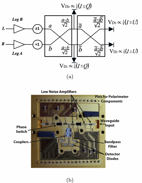
Figure 15. (a) Signal processing schematic for an ideal module in a polarimeter assembly. The diode raw signals are given for the two (±1) leg B states, and for the leg A state fixed (+1). For simplicity, details of the three LNAs and bandpass filters are not shown. (b) Internal components of a 5 cm × 5 cm Q-band module.
Download figure:
Standard image High-resolution imageTable 8 shows the idealized detector diode outputs for the two states of leg B with the leg A state held fixed. The diode outputs are averaged and demodulated by additional warm electronics (see Section 6). Given a diode output of I ± Q(U), the averaging and demodulation operations return I and Q(U), respectively.37 The Stokes parameters can be self-consistently expressed in units of temperature as follows (Staggs et al. 2002). Let Tx (Ty) be the brightness temperature of a source that emits the observed value of  (
( ). The Stokes parameters in temperature units become
For completeness, the voltage VQ1 appearing at the Q1 diode would measure
where ± indicates the states of leg B, and g is the responsivity constant extracted using calibration tools and procedures described in Sections 7 and 8.
Table 8. Idealized Detector Diode Outputs for a Polarimeter Assembly
| Diode | Raw Output | Average | Demodulated |
|---|---|---|---|
| D1 |  |
∝  |
∝  |
| D2 |  |
∝  |
∝  |
| D3 |  |
∝  |
∝  |
| D4 |  |
∝  |
∝  |
Note. Results are shown for the two states of leg B, with the leg A state held fixed.
Download table as: ASCIITypeset image
In practice, the phase of leg B is switched at 4 kHz, reducing the 1/f knee frequency from the LNAs once the signal is demodulated in the Q and U outputs (this is discussed in greater detail in Section 8.7). The choice of circularly-polarized inputs thus allows for the simultaneous measurement of both Stokes Q and U from differencing the same detector diode, giving an advantage in reduced systematic errors and typically lower knee frequencies over current incoherent detectors. However the phase switches do not reverse the sign of I; therefore the I output suffers from significant 1/f noise and so is not used to measure the temperature anisotropy.
The amplifier gains and transmission coefficients are represented by the proportionality symbols in Table 8. In practice, the transmission through leg B is not exactly identical between the two leg B states, leading to additional free parameters needed to characterize the module. If the leg B transmission differences are not accounted for, they lead to instrumental (i.e., false) polarization. This is resolved by modulating the phase of leg A at 50 Hz during data taking, and performing a double demodulation procedure on the offline data. Imperfections in the optics and the septum polarizer introduce additional offsets and terms proportional to I. These effects are discussed in Appendix B.
In practice, the signal pseudo-correlation is implemented in a single small package as shown in Figure 15(b) (Kangaslahti et al. 2006; Cleary 2010). The LNAs, phase switches and hybrid couplers are all produced using Indium–Phosphide (InP) fabrication processes. Three LNAs, each with gain ∼25 dB, are used in each of the two legs. When the input amplifiers are packaged in individual amplifier blocks and cryogenically cooled to ∼20 K, they exhibit noise temperatures of about 18 K (50–80 K) for the Q-band (W-band). The phase switches operate by sending the signal down one of two paths within the phase switch circuit, one of which has an added length of λ/2 (i.e., 180° shift). Two InP PIN (p-doped, intrinsic-semiconductor, n-doped) diodes control which path the signal takes. The signals go through band-defining passive filters made from alumina substrates, and are then detected by commercially-available Schottky detector diodes downstream of the hybrid couplers. The amplifiers and phase switches are specific to each band, and hence unique to each array. The detector diodes are capable of functioning at both 40 GHz and 90 GHz, and so are identical between the two arrays.
The module components are packaged into clamshell-style brass housings, precision-machined for accurate component placement and signal routing. To provide bias for active components and readout of diodes, the housing has feedthrough pins connecting to the module components via microstrip lines on alumina substrates and wire bonds. Miniature absorbers and an epoxy gasket between the two halves of the clamshell are used to suppress cross talk between the RF and DC components. All Q-band modules and roughly 40% of W-band modules were assembled by hand. For the remaining W-band modules, the components and substrates were automatically placed in the housings by a commercial contractor using a pick-and-place machine; the wire bonding, absorber and epoxy gasket were then finished by hand.
5.3. Differential-temperature Assemblies
The differential-temperature assemblies are grouped into pairs of assemblies, with waveguide components that mix two neighboring horn signals into two neighboring modules. Figures 16(a) and (b) show the schematic and implementation of these assemblies. An orthomode transducer (OMT) located after feed horn A outputs the linear polarizations EAx and EAy. One of these polarizations, EAy, enters a waveguide 180° coupler (a "magic-tee") and is combined with EBx from the adjacent feed horn. The magic-tee outputs are coupled to a module's inputs. The OMTs were reused from CAPMAP (Barkats et al. 2005) while the waveguide routing and magic-tees were made by Custom Microwave, Inc. Note that the differential-temperature assembly design resembles that of WMAP (Jarosik et al. 2003b), with the significant differences being in the feed horn separation and the implementation of the LNAs, both due to advances in MMIC HEMT LNAs and planar circuitry that enabled QUIET's cryogenically cooled integrated compact array design.
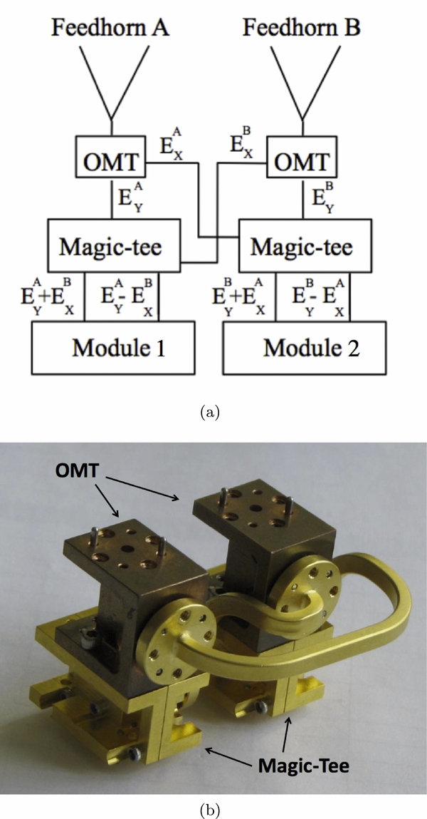
Figure 16. (a) Schematic of the waveguide coupling for the differential-temperature assembly. An Orthomode Transducer (OMT) located after feed horn A outputs the linear polarizations, EAx and EAy. One of these polarizations, EAy, enters a magic-tee 180° hybrid coupler and is combined with the orthogonal polarization from an adjacent feed horn, EBx. The factors of  for the magic-tee output labels have been omitted for simplicity. (b) Implementation of a W-band differential-temperature assembly (modules and feed horns not shown).
Download figure:
Standard image High-resolution imageFor an ideal differential-temperature assembly, the demodulated Q diodes (D1 and D4) measure  , while their counterparts in the adjacent differential-temperature assembly measure
  . The difference of demodulated Q diode outputs from adjacent differential-temperature assemblies measure the beam-differenced total power
  (see Table 9). The demodulated U diodes (D2 and D3) would measure zero for an ideal assembly. However, frequency-dependent unequal path lengths (ϕ) in the two legs of a module mix some of the temperature difference signal from the Q diodes (mixing ∝cos (ϕ)) to the U diodes (mixing ∝sin (ϕ)). We measure ∼15–30% of the signal on the U-diodes (ϕ ∼ 10°–20°).
Table 9. Idealized Detector Diode Outputs for a Differential-temperature Assembly
| Mod 1 | Mod 2 | |
|---|---|---|
| D1 |  |
 |
| D4 |  |
 |
| demod(D1, Mod1) − | ||
| demod(D1, Mod2) |  | |
Notes. Outputs of D1 and D4 corresponding to a leg B state of +1(− 1), with leg A fixed at +1. Also shown is the difference of the demodulated D1 signals from two modules. The outputs of D2 and D3 are zero for an ideal assembly (see the text).
Download table as: ASCIITypeset image
Finally, we note that the sum of demodulated Q diode outputs from adjacent modules is QA + QB, where Q is the Stokes Q parameter seen by the respective horns. Thus one can in principle extract polarization information from the differential-temperature assemblies. However, as these assemblies form a small fraction of the array, the sensitivity gain is marginal and so this was not explored further in the analyses.
6. ELECTRONICS
Downstream of the modules are electronics for detector biasing, timing, preamplification, digitization, and data collection. These functions are accomplished by four systems: (1) Passive Interfaces, (2) Bias, (3) Readout, and (4) Data Management. The Passive Interfaces system (Section 6.1) forms the interface between the modules, the Bias system, and the Readout system. The Bias system (Section 6.2) provides the necessary bias to each module's active components. The Readout system (Section 6.3) amplifies and digitizes the module outputs. The Data Management system (Section 6.4) commands the other systems and records the data. The Bias and Readout systems are housed in a weather-proof temperature-controlled enclosure to protect them from the harsh conditions of the Atacama Desert. The enclosure also serves as a Faraday cage to minimize radio-frequency interference. Further description of these electronics can be found in Bogdan et al. (2007).
6.1. Passive Interfaces
The electrical connection to, and protection of, the modules is provided by Module Assembly Boards (MABs). Each MAB is a printed circuit board with pin sockets for seven modules. Voltage clamps and RC low-pass filters protect the sensitive components inside the module from damage. The Q-band (W-band) modules require 28 (23) pins for grounding, biasing active components, and measuring the detector diode signals. All of these electrical connections are routed to the outside the cryostat. After the MAB protection circuitry, these signals travel on high density flexible printed circuits (FPC), which bring them out of the cryostat through Stycast-epoxy–filled hermetic seals. An additional layer of electronic protection circuitry is provided by the array interface boards, which also adapt the FPC signals to board-edge connectors and route to the Bias and Readout systems.
6.2. Bias System
All biasing is accomplished by custom circuit boards. The amplifier bias boards provide voltage and current to power the amplifiers in the modules. Each of these bias signals is controlled by a 10-bit digital-to-analog converter (DAC), which allows the biases to be tuned for optimal performance of each amplifier. Phase switch boards provide control currents to the PIN diodes in the phase switches. The control current is switched by the board at 4 kHz for one phase switch and 50 Hz for the other phase switch, generating the modulation described in Section 5.2. The data taken during the switch transition time are discarded in the Readout system. A housekeeping board monitors the bias signals at ∼1 Hz for each item being monitored. The housekeeping board multiplexes these items, switching only during the phase switch transitions when data will be discarded.
The Q-band amplifier bias boards are designed to operate at 25°C so the enclosure is thermally regulated at that temperature. The W-band amplifier bias boards use a different design that is much less temperature sensitive. Therefore, the enclosure regulation was less strict and the temperature was allowed to vary between 35°C and 40°C, depending on the time of year, to reduce the power needed for regulation. For both the Q-band and W-band observing seasons, the enclosure temperature remained within the regulation setpoint for ∼90% of the time. For the Q-band system, the excursions primarily affect the drain-current bias supplied by the amplifier bias boards, which changes the detector responsivity by ∼2%/°C. This effect is taken into account with an enclosure-temperature dependent responsivity model (QUIET Collaboration et al. 2011).
6.3. Readout System
The Readout system first amplifies each module's detector diode output by ∼130 in order to match the voltage range of the digitizers. The noise of this warm preamplifier circuit does not contribute significantly to the total noise. This is determined in situ at the site by selectively turning off the LNAs in the module and seeing that the total noise decreases by roughly two orders of magnitude. For the W-band array, the preamplifier noise contributes less than 2% to the total noise in the quadrature sum. The amplifier chain also low-pass filters the signal at ∼160 kHz to prevent aliasing in digitization. Each detector diode output is digitized by a separate 18-bit Analog Devices AD7674 (Analog–Digital Converter) ADC with 4V dynamic range at a rate of 800 kHz. Each ADC Board has a field-programmable gate array (FPGA) that accumulates the samples from the 32 ADCs on that Board. The FPGA on one ADC Board, designated the "Master ADC Board," generates the 4 kHz and 50 Hz signals used by the Bias system to modulate the phase switch control currents. This signal is also distributed to all ADC Boards, and the FPGA on each ADC Board uses it to demodulate the detector diode data synchronously with the phase switch modulation.
Figure 17 summarizes the organization of data performed by the FPGA. The FPGA organizes the 800 kHz detector diode data into continuous 10 ms blocks (i.e., 100 Hz time streams), itself organized into continuous 125 μs blocks. These 10 ms blocks contain an equal sampling of both 4 kHz clock states. In the "TP" stream, the 800 kHz data within a 10 ms block are averaged, regardless of the 4 kHz clock state. This stream is sensitive to Stokes I and is used for calibration and monitoring. In the "demodulated" stream, data within a 125 μs block have the same 4 kHz phase state, and are averaged. Averaged data from sequential 125 μs blocks are differenced, thus forming the polarization-sensitive data stream. Offline, two adjacent 10 ms blocks in the demodulated stream are differenced to form the "double-demodulated" (50 Hz) stream. The W-band ADC firmware was upgraded to include an additional specially demodulated 100 Hz data stream, called the "quadrature stream." Unlike the usual demodulated stream, data within a 125 μs block populate equally both 4 kHz phase states, and are averaged. When these averaged data are differenced, the result has the same noise as demodulated data but has no signal. The quadrature stream is used to monitor potential contamination and to understand the detector noise properties.
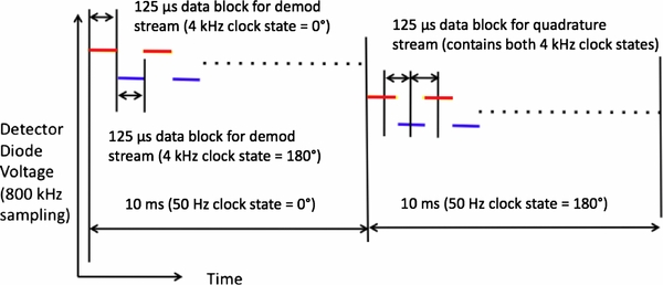
Figure 17. Organization of 800 kHz data to form the demodulated and quadrature 100 Hz streams. The blue and red lines show detector diode data for the two 4 kHz phase states. Levels are exaggerated for clarity.
Download figure:
Standard image High-resolution imageAs noted earlier, the data are masked at the phase switch transition. Masking 14% of the samples around the transition is found to be adequate to remove contamination in the data stream.
The ADC Boards have a small nonlinearity in their response. At intervals of 1024 counts, the ADC output has a jump discontinuity between 1 and 40 counts, affecting ∼14% of the data. This jump is shown schematically in Figure 18. When the 800 kHz data stream value falls at a discontinuity, the jump in the output signal will trickle into the 100 Hz stream. This nonlinearity is corrected in the 100 Hz stream. The correction is statistical in nature, based on the width of the 800 kHz noise and its proximity to the discontinuity (Bischoff 2010). This nonlinearity, if uncorrected, causes a variation of responsivity during a CES and a systematic effect similar to the leakage of temperature to polarization. For the Q-band, the correction reduces the ADC nonlinearity to contribute at most 3% to the leakage bias systematic error, and at most 50% to the CES responsivity systematic error. For the W-band, the residual ADC nonlinearity adds 40% in quadrature to the leakage bias systematic error. The effect on the CES responsivity is <1%, negligible compared with other errors in the gain model. These affect r at a level below 0.01 for the W-band.
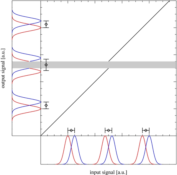
Figure 18. Nonlinear response of the ADC plotted in arbitrary units. The horizontal axis shows the ADC input near the discontinuity. The red and blue distributions show the fluctuations of 800 kHz samples in two different 4 kHz phase switch states. When these distributions cross the ADC response discontinuity, the output distributions are split at the discontinuity. When the red and blue states are differenced to create demodulated data, the split caused by the discontinuity is added to the result.
Download figure:
Standard image High-resolution imageThe Readout system ensures that the housekeeping data and 100 Hz data from the detectors are synchronized to each other and to the mount motion encoder readout. Synchronization is achieved by distributing the same GPS-derived IRIG-B38 time code to both the receiver and mount electronics. In the Readout system, the time code is decoded by a Symmetricom TTM635VME-OCXO timing board. Clock signals of 1 Hz and 10 MHz, locked to the IRIG-B time code, synchronize the readout of all ADC Boards. The timing board provides the GPS-derived time to the Data Management system so that each datum is assigned a time stamp.
6.4. Data Management
The Data Management system sends commands to the Bias system to prepare for observation, acquires the data from the Readout system, writes them to disk, and creates summary plots of the detector diode signals and housekeeping data for display in real time. The complete data are written to disk and DVDs in the control room at the observation site at a rate of ∼8 GB day−1 for the Q-band array. W-band array data are written to blu-ray optical discs at a rate of ∼35 GB day−1. A subset of ∼10% of the data were transferred by internet every day to North America for more rapid analysis and monitoring. The DVDs or blu-ray discs were mailed weekly to North America.
7. ARTIFICIAL CALIBRATORS
Both astronomical and artificial calibrators are used to characterize the instrument. Astronomical calibrators are described in Sections 3.4 and 8. This section focuses on the artificial calibrators developed for QUIET for use in the laboratory and at the observation site.
7.1. The Optimizer
The polarized response of the receiver in the laboratory is measured with the "optimizer," a reflective plate and cryogenic load that rotate around the boresight of the cryostat (Figure 19). The optimizer was used to verify that the responsivities derived from unpolarized measurements with cryogenic loads were not substantially different from the polarized responsivities, and hence that the projections of instrument sensitivity (which were made from unpolarized measurements) are valid for the Q-band array. For the W-band array, the optimizer was used to select functioning modules for the final array configuration.

Figure 19. Optimizer consists of a reflective metal plate and a cryogenic load, which corotate about the cryostat boresight axis. The plate angle is β, which was set to 45° in this case. The reflected signal is polarized (given by Equation (14)) and the polarized component modulates at twice the angular frequency of the rotating apparatus.
Download figure:
Standard image High-resolution imageThe plate is oriented at angle β from the plane of the feed horns and reflects radiation from the cryogenic load into the window of the cryostat. The resulting amplitude of the Stokes Q vector can be computed in temperature units via (Barkats et al. 2005):
where δ is the skin depth, ρ is the bulk resistivity of the metal plate, μ0 is the permeability of free space, ν and λ correspond to the center frequency and wavelength of the detector bandpass, t is time, and Tplate and Tload are the temperatures of the plate and cryogenic load. This apparatus rotates at an angular speed α around the boresight of the cryostat so that the resulting polarized signal will rotate between the Stokes Q and U at an angular speed of 2α. Polarization signals that do not rotate with the system (such as thermal emission from objects in the laboratory) will be detected at a rate of α, and so can be removed.
The predicted polarized emission from Equation (14) and the measured voltages on the detector diodes are used to calculate the polarized responsivities for polarimeters whose beams primarily sample the reflected cryogenic load. Various plate materials (aluminum, stainless steel, and galvanized steel) and two thermal loads (liquid nitrogen and liquid argon) are used to obtain multiple estimates of the polarized responsivity. The loads are too small to fill the entire array beam, so only the measurements from the central polarimeter (Q-band) or inner two rings (W-band) are used.
7.2. The Wire Grid Polarizer
A "sparse wire grid" (Tajima et al. 2012), a plane of parallel wires held in a large circular frame with the same diameter as the cryostat window, was used to impose and modulate a polarization signal onto the array. For the polarization parallel to the grid wires, a fraction of the rays that would ordinarily pass through the telescope to the cold sky are instead scattered to large angles, mostly terminating on the warm ground shield. The grid is placed as close to the cryostat aperture as possible to minimize interference with the telescope optics and to ensure that it covers the field of view of each detector (Figure 20).

Figure 20. Sparse wire grid array mounted on the W-band cryostat (right), and the fine wire detail (left). The grid rotates about the boresight axis of the cryostat at around 8 rotations per minute (RPM).
Download figure:
Standard image High-resolution imageWith this geometry, the polarized signal directed parallel to the wires is empirically found to be ∼2 K. The circular frame rotates about the cryostat boresight axis via a small motor, allowing for modulation of the injected polarized signal at a constant frequency. The wire grid was used for calibration measurements in the laboratory and three times during the observing season: at the end of the Q-band observing season and at the beginning and end of the W-band season. The grid was not mounted on the cryostat during sky observations.
An example of the data taken with the rotating grid is shown in Figure 21. In the ideal case in which the intensity of the reflected radiation is isotropically uniform over the array, the polarized signal D(θ) from each detector diode would exhibit a sinusoidal dependence at twice the frequency of θ, the angle about the cryostat boresight axis between the wires and a fixed point on the cryostat. The measured polarization signal has an additional dependence on θ due to rays terminating at different temperatures in the non-uniform ground screen. This variation appears in both the polarized data stream D and the total power data stream I as a function of θ, and so this variation can be measured in the I data stream and accounted for in the D data stream. Each detector diode data stream is fitted to the form

where D(θ) and I(θ) are the double-demodulated polarization and total power signals, respectively. Here, I0 is the average of I(θ) over all angles θ, and D0 is an offset term discussed in Appendix B.1. The fit extracts γ, the angle θ that maximizes D(θ), D2, the polarization amplitude (in mV), and η, a dimensionless constant relating the total power to polarization responsivity. Since the fixed point on the cryostat used to define θ can be arbitrarily chosen, only the relative γs amongst the detector diodes are relevant; they are just the relative detector angles. The values of D2 indicate the spread of polarized responsivities. For the W-band, their relative ratios agree with ones derived from Tau A observations at the level of 20%. The precision of this agreement is limited by the statistical errors of Tau A observations for the off-center detectors.
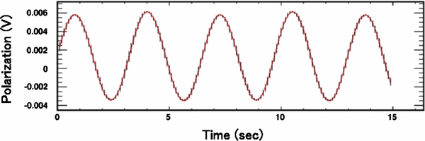
Figure 21. Polarization response of a detector as a function of time, where the wire grid was rotating at ∼8 RPM. A sinusoidal response is clearly observed at twice the rotation frequency. The curve is the fit to the data (dots) using Equation (15).
Download figure:
Standard image High-resolution image8. RECEIVER CHARACTERIZATION AND CALIBRATION
Each receiver diode (Table 10) is characterized by its bandpass, noise level, polarization angle, and total power and polarized responsivities. Calibration of the polarization, total power, and differential-power data products was performed in the laboratory prior to deployment, and at the observing site with non-astronomical calibrators as well as two primary astronomical calibration data sets: polarized calibrators consisting of Tau A and the Moon; and unpolarized calibrators consisting of Jupiter, Venus, and sky dips. All calibration for the differential-temperature data was performed with special temperature calibration observations of Jupiter, Venus, and the Moon.
Table 10. Detector Yield for the Q-band and W-band Arrays
| Band | Q | W |
|---|---|---|
| Number of modules | 19 | 90 |
| Polarization modules | 17 | 84 |
| Polarization diodes | 68 | 336 |
| Working polarization diodes (Stokes Q) | 31 | 153 |
| Working polarization diodes (Stokes U) | 31 | 155 |
| Differential-temperature modules | 2 | 6 |
| DT diodes (Stokes Q only) | 4 | 12 |
| Working DT diodes (Stokes Q only) | 4 | 12 |
Download table as: ASCIITypeset image
Calibration measurements from the polarization and total power data streams from the polarimeter modules were used to calibrate all of the polarization data. The total power stream was used for weather monitoring, assessing rapid responsivity variations on time scales around a CES length (Q-band only), and to understand the polarized beam measurements (Section 3.4). While data from the differential-temperature assemblies was not necessary to calibrate the polarization channels, we used it to check pointing and inform limits on instrumental systematics for the polarimeter data, primarily for responsivity. For the Q-band receiver, the beam shape and solid angle from the differential-temperature modules were used to estimate the systematic errors on the responsivity, conservatively assuming that the differences in beam solid angle were due to location on the focal plane (the differential-temperature assemblies are located on the edge of the array) and not from intrinsic beam differences between the polarization and differential-temperature optical chains (QUIET Collaboration et al. 2011). The differences between the measured beams for the polarized assemblies and the beam differenced total power beams were used to provide systematic errors for the W-band window functions.
This section describes methods of module bias optimization (Section 8.1) and module leakage remediation (Section 8.2) as well as characterizing module bandpasses (Section 8.3), responsivities (Section 8.4), detector angles (Section 8.5), noise measurements (Sections 8.7 and 8.8), and sensitivity (Section 8.9).
8.1. Detector Biasing and Optimization
For the Q-band array, the amplifiers were biased manually for each module using a room temperature blackbody load in front of the cryostat. The phase switches were turned on separately, so that the signal only propagated through the module leg with the phase switch on. The bias values for the phase switches were chosen to equalize the signal measured on the two separate legs of the module, to keep the contribution to the module noise from the first-stage amplifier low, and for an adequate signal level, which should not compress the amplifiers. These bias settings were chosen once at the beginning of the season, and kept fixed during the observing season.
For the W-band array, biasing the modules by hand was not feasible due to the large number of modules compared with the Q-band array, and so an automatic method was developed. A sinusoidal polarized signal was injected during module biasing by continually rotating the sparse wire grid. Amplifier bias settings were found by maximizing the amplitude of the sinusoid relative to the time-stream noise. The bias settings were sampled via a computer-based downhill simplex algorithm and optimum values were found for all modules within a few hours. As with the Q-band array, the bias settings were kept fixed during the W-band observing season. Because the settings were chosen to enhance signal-to-noise ratio, balance between the legs was not explicitly prioritized (the consequences of this are discussed in the next section).
8.2. Temperature to Polarization Leakage Remediation
One source of leakage from total power into polarization from the module stems from differential power transmission between the two phase switch states within a given leg (Appendix B). We found that double demodulating (described in Section 5.2) typically reduced the root-mean-square of leakage from 0.8% to 0.4% for the W-band modules (Figure 22). The improvement was smaller for the Q-band array, <0.1%, likely because it was dominated by other sources of leakage (Sections 3.6 and 5.1) and because the phase switches had been balanced during bias optimization.
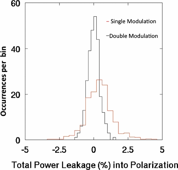
Figure 22. Histogram of diode leakage values between total power and polarization channels during a large angle sky dip for the W-band array before and after double demodulation. Double demodulating reduces the total power leakage by a factor of ∼2 for the W-band array.
Download figure:
Standard image High-resolution imageThe module is not the only source of leakage between temperature and polarization. Instrumental polarization from the mirrors, window, horns, etc. can be calibrated from large and small sky dips (elevation nods of ±20° and ±3° amplitude) with 0.3% precision for each sky dip as the signal from the changing atmospheric temperature leaks into the polarized data stream. The median monopole leakage was 0.2% for the W-band array, which is consistent with leakage measurements from Jupiter (Section 3.6). The median monopole leakage was 1.0% and 0.2% for the Q-diodes and U-diodes for the Q-band array, respectively, which are also consistent with measurements from other calibrators. The discrepancy in the monopole leakage between the two diodes for the Q-band array was anticipated from the measurements of the septum polarizers (Section 5.1).
8.3. Bandpasses
Typical bandpasses for the Q-band and W-band arrays are shown with the spectrum of the atmosphere in Figure 2. Central frequencies and bandwidths are computed from discrete frequency steps as


where Ii is the measured intensity from a detector diode for each frequency, νi, and Δν is the frequency step of the signal generator (100 MHz).
For the Q-band array, bandpasses were measured for each diode in the laboratory during the course of array testing and in end-of-season calibration measurements at the site. The laboratory measurement was performed by injecting a polarized carrier-wave signal from a signal generator with a standard-gain horn over a 35–50 GHz range. The signal was injected into the receiver array through the cryostat window without additional imaging optics, with the horn approximately 3 m away from the window. Sweeps were performed at least eight times. The average bandwidth and central frequency of the polarization modules are given in Table 11. The statistical errors on this measurement are obtained by finding the standard deviation between the eight measurements for a given module, and then averaging that standard deviation for all modules.
Table 11. Average Bandwidths and Central Frequencies for the Q-band and W-band Arrays
| Band | Bandwidth (GHz) | Central Frequency (GHz) | ||||
|---|---|---|---|---|---|---|
| Value | Stat. Error | System. Error | Value | Stat. Error | System. Error | |
| Q | 7.6 | 0.5 | 0.6 | 43.1 | 0.4 | 0.4 |
| W | 10.7 | ⋅⋅⋅ | 1.1 | 94.5 | ⋅⋅⋅ | 0.8 |
Download table as: ASCIITypeset image
Bandpasses were also measured at the site for the Q-band array by reflecting the swept signal from a small (∼1 cm2) plate into the primary mirror. While measurements performed in the laboratory and at the site are consistent with each other, the variation in bandpass shape between the two days of data taking at the site showed that the systematic errors were larger in the experimental setup at the site, so laboratory measurements were used where available. Although the amplifier bias settings were different between the laboratory and the site measurements, a review of laboratory measurements revealed that changing the amplifier bias over the range of interest had no significant effect on the bandpasses. The systematic error in Table 11 is the average of the difference between the site and lab bandpasses.
For the W-band array, bandpasses were measured at the site at the end of the observing season and the central frequency and bandwidth are also given in Table 11. A standard-gain horn was mounted beside the secondary mirror, so it could illuminate the cryostat window from ∼1.5 m away. The signal generator was swept over 72–120 GHz, while the phase switches were held constant (no switching). In this configuration the signal can be sent down each module leg separately. The responses at each frequency bin for each module leg were combined to emulate the power combinations occurring in the module:

where PA and PB are the measured bandpasses for the signal traveling through module legs A and B, respectively, ϕ is the detector angle (for example, a Q diode might have ϕ = 90° and a U diode might have ϕ = 45°), and γ is the angle of the polarized input from the signal generator. The measured signal is only dependent on the difference between the two angles. Systematic errors have two main sources: the accuracy with which the spike that was used to indicate the beginning of a sweep can be detected, and from reconstructing the bandpass for both module legs biased from data in which only one leg is biased. The first was computed by noting that the timing was accurate to 1.5 ms, which corresponded to 0.7 GHz during the sweep measurement. The second was computed by comparing measurements performed with both legs biased and the reconstruction from single-leg bandpasses from the total power stream. Because the total power stream does not have a dependence on detector angle ϕ, the two should be identical and the difference represents the systematic error in the measurement. The systematic error was found to be 0.3 GHz for the central frequency and 0.9 GHz for the bandwidth.
8.4. Responsivities
The responsivities were characterized for the differential-temperature modules and the polarization modules separately with different calibration sources. Responsivities of the differential-temperature modules are computed from calibration observations of Jupiter, RCW38, and Venus, one of which was observed ∼once per week for the Q-band receiver, and once a day for the W-band receiver. The responsivities could depend on the temperature of the bias boards, as described in Section 6.2, and so a temperature dependent responsivity model was developed for the Q-band receiver (QUIET Collaboration et al. 2011) and was found to be negligible for the W-band system (QUIET Collaboration et al. 2012).
For the Q-band array, the absolute polarimeter responsivity for the central horn was determined from Tau A measurements performed every two days. Relative responsivity values among the polarization modules were measured from observations of the Moon (performed once per week). Sky-dip measurements (elevation nods of ∼6° for "normal" sky dips, and ∼40° for "large" sky dips) are also used to obtain the relative total power responsivities of both the differential-temperature and polarized modules before each CES for the Q-band array ("flat fielding"). These frequent (once every ∼1.5 hr) responsivity measurements provide relative responsivity tracking for the differential-temperature and polarized modules on short time-scales. The relative responsivities were checked with an end-of-season wire grid measurement and measurements of Tau A with off-center modules. For the W-band array, the Moon is too bright for relative responsivity calibration, so measurements from the wire grid and Tau A from off-center modules were used.
One potential concern when using amplifiers is signal compression: an input-dependent responsivity that is greatly reduced at high input powers. Compression is typically manifested as different responsivity values for different load temperatures. For an ideal radiometer, the combination of sky temperature and typical measurement signals will not compress the amplifiers. However, calibration sources are typically much warmer than the CMB and so compression can have important consequences when deriving responsivities from astronomical or other sources (for example, the Moon is ∼223 K; Ulich et al. 1973). For the Q-band array, responsivity measurements in the laboratory and at the site with different calibration sources were all consistent with each other, confirming that the modules were not operating in a compressed regime. Laboratory responsivity studies of the W-band modules using liquid nitrogen as a cold load showed some evidence for compression. In the field, the W-band modules exhibited compression during observations of the Moon. The emission from the ∼05 Moon varies across its face (Ulich et al. 1973); polarized responsivities for a single detector could vary between the brightest and darkest portions of the Moon's face by 20% (worst case 50%). Ultimately this meant we could not use the Moon to calibrate the responsivities for the W-band receiver as we could with the Q-band receiver or we would have misestimated our responsivity (and hence our noise) by at least 20%.
Compression affects the polarized signal and the total power signal differently (Appendix A). Since the sky dips measure total power responsivity only, this complicates the use of sky dips to track relative polarized responsivity for the W-band array. As a result, daily Tau A measurements of the central module were used to measure fast variations. Relative responsivities between the central module and the other modules are obtained from additional Tau A measurements and an end-of-season polarization grid measurement and these were used to extrapolate absolute responsivities to all modules. The resulting instrumental systematics from using a single module to track fast variations is discussed in QUIET Collaboration et al. (2012).
Additional laboratory studies performed after deployment explain why the W-band modules were operated in a compressed regime: passive hybrids in the W-band modules had as much as twice the expected loss. To compensate for this loss, the amplifiers were biased for higher gain to overcome the post-detector noise. As a result, the gain was large enough that it contributed a significant fraction of the power required to compress the amplifiers. Modules with new passive components having lower loss have been produced. These modules exhibit little compression and have noise temperatures closer to the ∼50 K intrinsic W-band amplifier noise (Reeves 2012). This indicates we can gain a factor of two in sensitivity for W-band modules with the new, less lossy components.
8.5. Detector Angles
Absolute polarized detector angles were measured for the central module of each array through observations of Tau A, whose position angle is known to 02 precision from IRAM measurements (Aumont et al. 2010). For the Q-band array, the absolute angle shifted by as much as 2° due to jumps in the deck position during the first half of the Q-band season due to slippage in the deck encoder. The systematic uncertainties related to the encoder jumps are discussed in QUIET Collaboration et al. (2011). The Q-band angle calibration relied on weekly Moon observations and an end-of-season sparse wire grid measurement to find the relative angles of the diodes. The relative angles between one of the diodes of the central module and every other diode from all ∼35 Moon measurements deviated less than 02 from nominal, indicating that the relative angles remained nearly constant during the season. Relative detector angles are not affected by the encoder jumps.
The W-band array had a smaller, more efficient Tau A scan trajectory and was able to make measurements with all modules over the course of the season to obtain absolute angle calibration. The variance of detector angles for the central module from repeated measurements of Tau A is 03. The relative angles among the diodes were confirmed with end-of-season wire grid measurements for both arrays to within 09.
Relative angles for all diodes in the W-band array are shown in Figure 23. Systematic errors in the absolute angle are the largest source of systematic errors for the W-band array, which would limit the measurement of r to 0.01 at ℓ ∼ 100 (QUIET Collaboration et al. 2012).
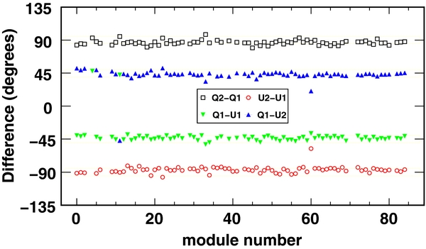
Figure 23. Detector angle differences among diodes for each module in the W-band array.
Download figure:
Standard image High-resolution image8.6. Pointing
The telescope pointing model is derived by fitting a physical model of the three-axis mount and telescope to astronomical observations (Næss 2012). The orientations of individual feed horns are determined by observations of the Moon and Jupiter. Then, holding the focal plane layout fixed, the parameters of the dynamical mount model are determined from observations of Jupiter, Venus, RCW38 (W-band only), and the Galactic plane.39 Optical observations are taken regularly with a co-aligned star camera and used to monitor the time evolution of the pointing model. Except for the mechanical problem with the deck-angle encoder during the first two months of Q-band observations (QUIET Collaboration et al. 2011), no significant trends are found.
The residual scatter after all pointing corrections is 35 rms in the Q-band observations (QUIET Collaboration et al. 2011) and 51 FWHM (22 rms) in the W-band observations (QUIET Collaboration et al. 2012). The larger residuals compared with the beam size in the W-band pointing could not be modeled from our pointing variables, but we explicitly account for them in the window function for the high-resolution W-band data, as described in QUIET Collaboration et al. (2012), where we also show that this is a negligible contribution to the constraint on r. In order to validate the pointing model, a high-resolution W-band map of PNM J538-4405 (Gold et al. 2011; a particularly bright point source in the QUIET observing field CMB-2) was produced and both its apparent position and angular size was found to be consistent with the assumed beam profile and estimated uncertainty.
8.7. Noise Spectra
Noise measurements at the site were obtained from a noise spectrum fit to the Fourier-transform of the double-demodulated time stream for each CES. The measured noise floor should be proportional to the combination of module noise temperature, atmospheric temperature, contributions from optical elements, and CMB temperature. A power law with a flat noise floor was assumed for the functional form of the noise spectrum,

where N(ν) and σ0 have units  , ν is frequency, σ0 is the white noise level, α is the slope of the low frequency end of the spectrum, and νknee is the knee frequency. A typical noise power spectrum for a W-band module is given in Figure 24, which also shows the effects on the noise of demodulating and double demodulating the time streams. After double demodulation, the median knee frequency is 5.5 mHz (10 mHz) for the Q-band (W-band) array; thus the noise is white at the scan frequencies of the telescope, 45–100 mHz.

Figure 24. Typical noise spectra of a W-band module with no demodulation, single demodulation, and double demodulation. Double demodulation reduces the knee frequencies below the telescope scan frequencies.
Download figure:
Standard image High-resolution imageThe white noise is correlated among detector diodes within a given module. The correlation between Q and U diodes is expected (Bischoff 2010); the theoretical expectation and typical measured correlations are given in Table 12. The measured correlation coefficients are larger than theoretically anticipated; the source is unknown but could come from unequal transmission in the coupling hybrid in the module, or from leakage of the atmosphere causing residual 1/f noise. However, the noise correlation among diodes is easily treated in the data analysis (QUIET Collaboration et al. 2011), and more importantly does not impact the measured polarized signal, which is a difference between diode signals: (Q1 − Q2) and (U1 − U2).
Table 12. Predicted and Measured Correlation Coefficients among Diodes
| Diode × Diode | Design Value | Typical Measured Value | |
|---|---|---|---|
| Q Band | W Band | ||
| Q × Q | 0 | 0.23 ± 0.09 | 0.06 ± 0.19 |
| U × U | 0 | 0.22 ± 0.08 | 0.06 ± 0.21 |
| Q × U | 0.5 | 0.54 ± 0.08 | 0.48 ± 0.11 |
Note. The error for each measured value is the standard deviation of the correlation coefficients among modules.
Download table as: ASCIITypeset image
8.8. System Noise Temperature
The system noise is given by
where Tatm is the effective atmospheric temperature, Gatm = e−τ is the transmission through the atmosphere where τ is atmospheric opacity,  is the brightness temperature of the CMB, Tmodule is the noise temperature of a QUIET module, {TR, GR}, {TW, GW}, {TIR, GIR}, {TH, GH}, and {TSP, GSP} are the effective noise temperatures and gains for both reflectors (including ohmic and spillover contributions), window, IR blocker, horns, and septum polarizers, respectively (Table 13).
Table 13. Estimated Contributions to the System Noise
| Description | Q Band | W Band | ||
|---|---|---|---|---|
| Gain | Noise (K) | Gain | Noise (K) | |
| CMB+sky | 0.96 | 11.1 | 0.98 | 5.9 |
| Reflectors | 0.99 | 2.7 | 0.99 | 2.7 |
| Window | 0.99 | 2.8 | 0.983 | 4.8 |
| Horn | 0.99 | 0.2 | 0.99 | 0.2 |
| Septum polarizer | 0.9 | 2.5 | 0.9 | 2.3 |
| TOTAL | 0.83 | 19 | 0.85 | 17 |
| Measured Tsystem | ⋅⋅⋅ | 38 | ⋅⋅⋅ | 109 |
| Implied Tmodule | ⋅⋅⋅ | 15 | ⋅⋅⋅ | 77 |
Notes. The noise from each component has been divided by the gain of the previous elements in the optical chain. The values for the gain are not measured and are included for illustrative purposes; thus there are no associated error estimates. The atmospheric temperature and loss were computed for an elevation of 66° (the mid point of the CES elevation range), and a PWV of 1.2 mm (Q Band) and 0.94 mm (W Band). All ambient temperatures are taken as 270 K.
Download table as: ASCIITypeset image
The system noise can be found from the total power time streams taken during sky dips. During a sky dip, the sky temperature seen by the receiver changes with telescope elevation. Using an atmospheric model, the change in signal with this model-dependent change in sky temperature allows us to estimate the system noise. The contribution to instrument noise due to the module alone can be estimated by subtracting assumed or measured values for all other known instrument noise sources (Table 13). All components other than the modules are lossy; thus their noise temperatures are given by (1/G − 1) × Tphys, where G is the gain of the component and Tphys is its physical temperature. The full receiver noise was found to be 38 K for the Q-band system and 109 K for the W-band system, yielding extrapolated module temperatures of 15 K and 77 K for a Q-band and W-band module, respectively. Measurements of the Q-band amplifiers give noise values of ∼18 K; the most likely source of the discrepancy (that the module noise temperature is higher than a single LNA noise temperature) is that the loss in the septum polarizer was overestimated. Similar measurements for the W-band module give amplifier noise values of 50 K. The discrepancy between the W-band module and amplifier temperatures stems from operating them uncompressed in the laboratory (this is explained in greater detail in Section 8.4).
8.9. Instrument Sensitivity
The sensitivity for the polarization response, Spol (μKs1/2), is calculated as the ratio of the white noise level to the responsivity. For the Q-band array, after data selection (QUIET Collaboration et al. 2011), the sensitivity is 69 μK s1/2 corresponding to an average module sensitivity of 275 μK s1/2. For the W-band array, the array sensitivity is 87 μK s1/2 (QUIET Collaboration et al. 2012), corresponding to an average module sensitivity of 756 μK s1/2. A histogram of module sensitivity is shown in Figure 25. Both values are given in thermodynamic units, so that the power detected by the receiver has been corrected from a Rayleigh–Jeans approximation to correspond to fluctuations in the blackbody temperature of the CMB. Functionally this is performed by dividing by CRJ, which is 0.95 (0.79) for the Q-band (W-band) central frequencies. These values can be compared to the expected sensitivity per module, Spol, from the radiometer equation (Kraus 1986):

Using the measured values for Tsystem and the atmospheric gain, Gatm (Table 13), the bandwidths Δν (Section 8.3), the Rayleigh–Jeans correction CRJ for the CMB, and the fraction of the data masked during the phase switch transitions, fmask (14%; Section 6), sensitivity values of 310 μK s1/2 for the Q band, and 913 μK s1/2 for the W band were found. Errors in bandpasses and the atmospheric temperature contribute directly to the difference between the two methods of computing the sensitivity Spol. A potential explanation for the greater discrepancy between these methods for the W-band array (∼30%) compared with the Q-band (∼11%) array is that Trec is measured from the total power stream during sky dips, which could be compressed as much as 30% (Appendix A) in the W-band data stream. This compression inflates the noise temperature by the same compression factor, although does not impact the polarization stream.
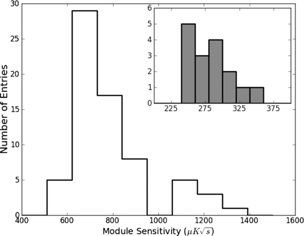
Figure 25. Histogram of module sensitivities for the W-band (main figure) and Q-band (inset) modules. The less sensitive modules have only two or three detector diodes functional.
Download figure:
Standard image High-resolution image9. CONCLUSIONS
QUIET employs the largest HEMT-based receiver arrays to date. The 17-element Q-band array has a polarization sensitivity of 69 μK s1/2, currently the most sensitive instrument in this band. The 84-element W-band array has a 87 μK s1/2 sensitivity. Together the two arrays give the instrument sensitivity to angular scales ℓ ∼ 25–975.
The instrument design also achieves extremely low systematic errors. The optical design uses high-gain, low-cross-polar, and low-sidelobe corrugated feed horns and septum polarizers. The receiver and mirrors are housed in an absorbing ground shield to reduce sidelobe pickup, and are mounted on a three-axis telescope with boresight rotation. The polarimeter assemblies use electronic double demodulation to reduce 1/f noise by a factor of ∼2–3 in the signal band and monopole leakage by a factor of ∼2 in power for the W-band receiver, with no additional complexity (since the differencing is done electronically) and in fact reduces the data computation burden by a factor of two by halving the data set size. Finally, the differential-temperature assemblies and calibration tools provide critical measurements and cross checks of the systematic errors. The dominant systematic errors at ℓ ∼ 100 are leakage for the Q-band instrument, and detector angle calibration for the W-band instrument. QUIET's Q-band result has a systematic error of r < 0.1 at ℓ = 100 (QUIET Collaboration et al. 2011), and r < 0.01 for the W-band result (QUIET Collaboration et al. 2012), the lowest systematic uncertainty on r published to date.
Support for the QUIET instrument and operation comes through the NSF cooperative agreement AST-0506648. Support was also provided by NSF awards PHY-0855887, PHY-0355328, AST-0448909, AST-1010016, and PHY-0551142; KAKENHI 20244041, 20740158, and 21111002; PRODEX C90284; a KIPAC Enterprise grant; and by the Strategic Alliance for the Implementation of New Technologies (SAINT). This research used resources of the National Energy Research Scientific Computing Center, which is supported by the Office of Science of the U.S. Department of Energy under Contract No. DE-AC02-05CH11231.
Some work was performed on the Joint Fermilab-KICP Supercomputing Cluster, supported by grants from Fermilab, the Kavli Institute for Cosmological Physics, and the University of Chicago. Some work was performed on the Titan Cluster, owned and maintained by the University of Oslo and NOTUR (the Norwegian High Performance Computing Consortium), and on the Central Computing System, owned and operated by the Computing Research Center at KEK. Portions of this work were performed at the Jet Propulsion Laboratory (JPL) and California Institute of Technology, operating under a contract with the National Aeronautics and Space Administration. The Q-band modules were developed using funding from the JPL R&TD program. We acknowledge the Northrop Grumman Corporation for collaboration in the development and fabrication of HEMT-based cryogenic temperature-compatible MMICs.
C.D. acknowledges an STFC Advanced Fellowship and an ERC IRG grant under FP7. R.B. acknowledges support from CONICYT project Basal PFB-06 and ALMA-Conicyt 31070015. A.D.M. acknowledges a Sloan foundation fellowship. H.K.E. acknowledges an ERC Starting Grant under FP7.
PWV measurements were provided by the Atacama Pathfinder Experiment (APEX). We thank CONICYT for granting permission to operate within the Chajnantor Scientific Preserve in Chile, and ALMA for providing site infrastructure support. Field operations were based at the Don Esteban facility run by Astro-Norte. We are particularly indebted to the engineers and technician who maintained and operated the telescope: José Cortés, Cristobal Jara, Freddy Muñoz, and Carlos Verdugo.
In addition, we acknowledge the following people for their assistance in the instrument design, construction, commissioning, operation, and in data analysis: Augusto Gutierrez Aitken, Colin Baines, Phil Bannister, Hannah Barker, Matthew R. Becker, Alex Blein, April Campbell, Anushya Chandra, Sea Moon Cho, Joelle Cooperrider, Mike Crofts, Emma Curry, Maire Daly, Fritz Dejongh, Joy Didier, Greg Dooley, Hans Eide, Will Grainger, Jonathon Goh, Peter Hamlington, Takeo Higuchi, Seth Hillbrand, Ben Hooberman, Kathryn D. Huff, Norm Jarosik, Eiichiro Komatsu, Jostein Kristiansen, Donna Kubik, Richard Lai, David Leibovitch, Kelly Lepo, Siqi Li, Martha Malin, Mark McCulloch, Oliver Montes, David Moore, Ian O'Dwyer, Gustavo Orellana, Stephen Osborne, Stephen Padin, Felipe Pedreros, Ashley Perko, Alan Robinson, Jacklyn Sanders, Dale Sanford, Yunior Savon, Mary Soria, Alex Sugarbaker, David Sutton, Matias Vidal, Liza Volkova, Stephanie Xenos, Octavio Zapata, and Mark Zaskowski.
APPENDIX A: COMPRESSION
This section explains some subtleties regarding nonlinearities, and how they affect the polarization and total power measurements differently. This complicates the use of periodic telescope sky dips to track the total power responsivity, which is assumed to also track the polarization responsivity. During CMB operations, the receiver load temperature varies by ∼2 K due to changes in the sky loading. Nonlinearities also affect the use of large sky dip and Moon signals to calibrate the total power responsivity. For HEMT LNAs, compression (in which the amplifier gain depends on the input signal level) is the nonlinearity that is typically encountered in the QUIET operating regime.
The effect of compression on polarization responsivity is analyzed here. Consider a horn looking at an unpolarized background at temperature T0, where T0 = T0x = T0y, with axes x and y defined by the septum polarizer. Given below are the Q1 diode measurements for the 0° and 180° leg B states, and the demodulated output (which is the polarization measurement):
where g0 is the gain at temperature T0.
Consider now the module observing a source and the background. Without loss of generality, let the source be polarized in the x direction at temperature T1 such that T1x = T0x + TSx, T1y = T0y, Tavg = (1/2) · (T0x + TSx + T0y). Then:
Note that the gain constant g1 is relevant for the temperature Tavg, for the following reason. Since the incident E-fields at the horn input are linearly polarized, the septum polarizer splits the power equally between legs A and B. Thus the legs see a constant input power given by Tavg, regardless of the instrumental position angle. Within the module, the LNAs are placed prior in the signal chain to any phase-sensitive circuitry. In this model, compression depends primarily on the input power at the first LNA. Therefore, the first LNA sees power represented by Tavg, so a gain g1 is associated to that input temperature. Thus, Equation (A2) shows that the polarization measurement is compressed by (g0 − g1)/g1. It is estimated that (g0 − g1)/g1 changes by roughly 0.1% per Kelvin for the W-band modules.
Now consider the effect of compression on the total power responsivity. For an unpolarized background source at temperature T0, the Q1 diode voltages for the leg B 0° and 180° states are as given in Equation (A1), and the average (which gives the total power) is

Similarly, an unpolarized background source at temperature T1 results in

Here, g1 and g0 are the gains for temperatures T1 and T0, respectively. It can be shown that
where c is the ratio between the observed signal difference and the expected difference without compression.
Comparing Equation (A5) with Equation (A2), the total power sensitivity compression is magnified by T0/(T1 − T0). Assuming as an example, T1 − T0 = 2 K (typical for a sky dip), a system temperature of T0 = 120 K, and a typical gain compression of (g0 − g1)/g1 = 0.002 over that range, the resulting ratio is c = 93%, or 7% signal loss. Therefore, in the data analysis, the absolute responsivities are derived from polarized source measurements to avoid systematic biases of this type for the W-band diodes.
APPENDIX B: DOUBLE DEMODULATION
This section discusses some imperfections in the module and their mitigation using double demodulation. Table 8 shows the detector diode outputs of an ideal module for the two leg B states, with the leg A state held fixed. The idealization (see Figure 15(a)) assumes equal transmission between the two leg B states, and between the two leg A states, and an ideal septum polarizer (see Appendix B.1). In practice, the transmissions are unequal, thus requiring extra parameters to describe the module. Without loss of generality, let the transmission through the 0°(↑) state of legs A and B be equal to unity, and define βA and βB to be the transmissions through these legs for the 180°(↓) state. Using gA and gB as the effective voltage gains of the two legs (see Figure 26), the detector diode voltages are given by
where the upper (lower) signs correspond to the signal of the diodes Q1 and U1 (Q2 and U2). The four rows for each Vi correspond to the phase switch states of (A, B) = (↑, ↑), (↑, ↓), (↓, ↑), and (↓, ↓), from the top to the bottom. Transmission imbalance between the phase switch states, signified by the deviation from unity of βA and βB, causes I → Q/U leakage. This can be seen in Table 14, showing the demodulated output dependences on  . However, the difference between the ↑ and ↓ demodulated outputs is free from I-dependence. Calculating the time series of this difference is referred to as double demodulation. For the W-band, the rms of I → Q/U leakage distribution is reduced from roughly 0.8% in the demodulated stream, to 0.4% in the double-demodulated stream. A smaller reduction of <0.1% is found for the Q-band, as the leakage is dominated by other effects.

Figure 26. Schematic of signal processing in a QUIET polarimeter assembly.
Download figure:
Standard image High-resolution imageTable 14. Expressions for the Demodulated Output
| Leg A | Demodulated | |
|---|---|---|
| Phase State | Diode | Output |
| ↑ | Q1 (Q2) |  |
| ↑ | U1 (U2) |  |
| ↓ | Q1 (Q2) |  |
| ↓ | U1 (U2) |  |
Notes. Demodulated signal for each leg A phase state with the leg B phase state switching at 4 kHz. A factor of 1/4 has been omitted from each expression. The terms involving Stokes V are also omitted for simplicity. The upper (lower) signs correspond to detector diodes Q1 and U1 (Q2 and U2).
Download table as: ASCIITypeset image
B.1. Polarimeter Assembly Offset and I → Q/U Leakage
As shown above, it can be assumed that the module does not generate any instrumental polarization on its own since the double demodulation procedure nulls out this effect. However, the interaction between the module and septum polarizer can cause irreducible instrumental polarization and offsets; this section derives these couplings. Since the module does not generate instrumental polarization on its own, the module measures:

and

where Lm and Rm are the signals transmitted into the module inputs. Without loss of generality, all the constant factors are absorbed into the responsivity and set to unity. The signals transmitted into the module inputs need not be the same as the L and R components at the septum polarizer input; this difference is a cause of instrumental polarization.
The effect of the septum polarizer is described by a 4 × 4 complex scattering matrix S:
where Ex and Ey are electric field components at the septum polarizer input port; L' and R' are the fields at the two septum polarizer output ports;  and
and  are the electric fields emitted from the septum polarizer back toward the feed horn; Lr and Rr are signals reflected (or emitted) from the module inputs traveling back toward the septum polarizer output ports; eiγ is the propagation phase shift; τij and r are transmission and reflection coefficients, respectively; c is a measure of the isolation between the output ports. For an ideal septum polarizer, τ = 1 and r = c = 0. Symmetry across the septum implies τ21 = τ31, τ24 = τ34, r2 = r3, and r41 = 0, although manufacturing errors can cause these conditions to be violated. As described in Sections 5.1 and 8, there are small departures from ideal operation. In this section these departures are computed up to second order. Note that the scattering matrix is frequency-dependent. The analysis given here is strictly for a single frequency. In practice, the result should be averaged with the effective bandpass. The median value of the Q(W)-band, band-averaged return loss (= −20log |r|) for the septum polarizers is 19(30) dB, while the median value of the Q(W)-band, band-averaged isolation (= −20log |c|) is 22(28) dB. Another quantity of interest is median value of the band averaged (linear) axial ratio of the septum polarizers. This is measured to be 1.12(1.07) for Q(W) band and implies a cross-polar discrimination of 24.9(29.4) dB.
A perturbative expansion is used to derive Lm and Rm which are the fields transmitted into the module inputs due to a sky source consisting of fields Ex and Ey. Here a noiseless module is assumed. The case of a noise signal from the module is described later. To lowest order, the S matrix applied to the column vector (Ex, 0, 0, Ey) yields (0, L', R', 0), where
Similarly,

where  and
and  . However, Lm and Rm differ from L' and R' due to reflection at the module input. Let rL (rR) be the reflection coefficient at the module's L (R) input. Then the S matrix applied to (Ex, rLL', rRR', Ey) yields (−, Lm, Rm, −) where


and for simplicity, the expressions for the first and fourth component are omitted. The module output is

where ri, c, rR and rL are assumed to be small, and terms above second order are dropped.
In the following, the right-hand side of Equation (B11) is simplified into the underlying physics parameters Q and U in order to identify the sources of instrumental polarization. The terms L'*L' and R'*R' need only be calculated to leading order since they appear in Equation (B11) multiplied by the second order terms crL and  . To leading order, L'*L' = L*L and R'*R' = R*R since τij ≈ 1.
The first term in Equation (B11) is expanded by substituting Equations (B7) and (B8) and using L*R = (Q − iU)/2, LL* = (I + V)/2, and RR* = (I − V)/2 to obtain
The first two terms are the expected response to Q and U. The presence of τij in these terms parameterizes the imperfections in the septum polarizer transmissions. These terms reduce the gain to Q and U, and in general cause mixing between Q and U. In practice, the gain is absorbed into the calibration of the total system responsivity,40 and the Q/U leakage is absorbed into the detector angle as defined in Equations (9) and (10). Therefore, these two terms do not cause instrumental polarization, and these imperfections can be neglected in the following discussion. By the same argument, the terms r3rR and  in Equation (B11) can be ignored since their only effect is to change the gain and detector angle.
The third and fourth terms represents I → Q/U and V → Q/U leakage, respectively. Since V ≪ I for reasonable sources and the coefficients have the same order, these circular polarization leakages are neglected. Combining these simplifications, the right-hand-side of Equation (B11) becomes:
where  and
and  . Using Equation (B3) and ignoring U → Q leakage, the module output is

where the first term is the expected response, the second term is I → Q leakage due to differential loss, and the third term is leakage caused by reflections at the module inputs coupling with the septum polarizer cross talk. Similarly, using Equation (B4) and ignoring the Q → U leakage:

In summary, the two equations above describe the measurements of a sky signal in the absence of noise from the module.
Now consider the case of noise emitted from the module inputs, reflecting from the septum polarizer and returning into the module. Module noise stems primarily from the HEMT-based first-stage LNAs. Since the sky signal and module noise are relatively incoherent, they decouple and the sky signal can be neglected in the following. Let the module noise fields be given by the column vector (0, Lr, Rr, 0). Applying the S matrix, the vector (−, Lm, Rm, −) is obtained where


The output is

because the LrRr terms average to zero due to the fact that the two amplifier noises are uncorrelated. Thus each output acquires an offset


The offset is independent of the input I; however, it is modulated by gain fluctuations so the offset also contributes to 1/f noise at a level suppressed by the product of the cross-talk and reflection coefficients in the OMT and so would not dominate.
Footnotes
- 30
Bruce Winstein, who died in 2011 February soon after observations were completed, was the principal investigator for QUIET. His intellectual and scientific guidance were crucial to the experiment's success.
- 31
- 32
The absorber is Emerson Cumming HR-10 (www.eccosorb.com) and is covered with Volara made by Sekisui Voltek (www.sekisuivoltek.com). The Volara is transparent at QUIET observing frequencies and acts as weatherproofing.
- 33
The detector diode nomenclature is described in Section 5.2.
- 34
For reference, when ϕd = 0° or ϕd = 180°,
 (defined in Section 3.5.3) is parallel to the ground. In the event that the parallactic angle of a given beam is similarly zero (so that the beam is observing the local meridian), then the plane is perpendicular to the local meridian, yielding an instrumental position angle ψ = 0°. The plane is coincident with the plane of the septum polarizers described in Section 5.1.
 - 35
- 36
The phase switch acts uniformly across the bandwidth of the module.
- 37
When referring to diodes D1, D2, D3, and D4, the naming convention Q1, U1, U2, and Q2 diodes respectively is used.
- 38
Inter-range Instrumentation Group Mod B.
- 39
For preliminary Galactic maps from QUIET, see Wehus (2012).
- 40
The effect of the gain difference on the leakage terms is a neglected higher order effect.


