


ABSTRACT
Analyses of exoplanet statistics suggest a trend of giant planet occurrence with host star mass, a clue to how planets like Jupiter form. One missing piece of the puzzle is the occurrence around late K dwarf stars (masses of 0.5–0.75 M☉ and effective temperatures of 3900–4800 K). We analyzed four years of Doppler radial velocity (RVs) data for 110 late K dwarfs, one of which hosts two previously reported giant planets. We estimate that 4.0% ± 2.3% of these stars have Saturn-mass or larger planets with orbital periods <245 days, depending on the planet mass distribution and RV variability of stars without giant planets. We also estimate that 0.7% ± 0.5% of similar stars observed by Kepler have giant planets. This Kepler rate is significantly (99% confidence) lower than that derived from our Doppler survey, but the difference vanishes if only the single Doppler system (HIP 57274) with completely resolved orbits is considered. The difference could also be explained by the exclusion of close binaries (without giant planets) from the Doppler but not Kepler surveys, the effect of long-period companions and stellar noise on the Doppler data, or an intrinsic difference between the two populations. Our estimates for late K dwarfs bridge those for solar-type stars and M dwarfs, and support a positive trend with stellar mass. Small sample size precludes statements about finer structure, e.g., a "shoulder" in the distribution of giant planets with stellar mass. Future surveys such as the Next Generation Transit Survey and the Transiting Exoplanet Satellite Survey will ameliorate this deficiency.
Export citation and abstract BibTeX RIS
1. INTRODUCTION
Parent star mass is a fundamental parameter in planet discovery space because there are both theoretical predictions and observational evidence that the properties of planetary systems depend on central star mass. In addition, it is of practical significance: the sensitivity of the Doppler, astrometric, and transit techniques of planet detection scale inversely with stellar mass (or radius), such that smaller planets can be detected around less massive stars (or smaller stars).
Most surveys for planets, i.e., ground-based radial velocity (RV) surveys and the Kepler transit survey mission, are flux- or magnitude-limited at visible wavelengths, favoring the inclusion of intrinsically bright stars. In addition, the Doppler method only works with spectra having large numbers of deep absorption lines, which disqualifies hot stars, and the transit method works better for cool dwarfs, around which planets produce deeper transits. These opposing trends mean that catalogs of exoplanet-hosting stars are dominated by solar-type stars with late F to early K spectral types (Udry et al. 2007; Batalha et al. 2010). Moreover, a focus on solar-mass stars satisfies a desire to determine the occurrence, nature, and potential habitability of planets around other stars like the Sun.
On the other hand, M dwarf stars are now widely recognized as an attractive "short cut" to the discovery of Earth-like planets because such stars are numerous, small, and their habitable zones are close-in, meaning that planets orbiting within them will be more detectable by the Doppler or transit methods. Doppler surveys have included the few nearby M dwarfs that are sufficiently bright at visible wavelengths (Bonfils et al. 2013), and high-precision infrared spectrographs are being constructed to take advantage of the greater emission of these stars at longer wavelengths (Artigau et al. 2011; Quirrenbach et al. 2012). Several thousand M dwarfs were added to the Kepler target catalog for these reasons (Batalha et al. 2010).
Between the early-K-type dwarfs and M dwarfs are the late K dwarfs, having K4–K7 spectral subtypes, Teff ≈ 3900–4800 K, and M* ≈ 0.5–0.75 M☉. These stars have been comparatively neglected in planet surveys because they are intrinsically faint and they are not M dwarfs. The two largest Doppler surveys, the California Planet Search (CPS) and the HARPS survey, include relatively few late K stars. Ironically, these stars may be especially attractive targets for Doppler surveys because intrinsic stellar Doppler noise or "jitter" decreases with later spectral type and could be <1 m s−1 among K dwarfs (Isaacson & Fischer 2010; Lovis et al. 2011). The K5 dwarf HD 85512 is one of the most Doppler-stable stars reported (residual rms = 0.75 m s−1), a property that has permitted the discovery of a super-Earth near or inside its habitable zone (Pepe et al. 2011).
Giant planets, defined here as planets with mass greater than that of Saturn (95 M⊕) or radius greater than 8 R⊕, are readily detected by Doppler observations with a sufficient time baseline if the planets orbit within ∼1 AU of their host stars. Their distribution with mass or spectral type of the host star can test the core accretion scenario of giant planet formation as well as models of orbital migration. Numerous studies have found evidence that the fraction of stars with giant planets increases with stellar mass (Fischer & Valenti 2005; Cumming et al. 2008; Johnson et al. 2010). Likewise, Fressin et al. (2013) estimated that the occurrence of giant planets is lower for Kepler M dwarfs than for G and K dwarfs. These findings support a theoretical prejudice that a more massive star is born with a more massive disk that can spawn the solid cores capable of accreting disk gas before its dispersal (Laughlin et al. 2004). However, any relation between disk mass and stellar mass is ambiguous (Williams & Cieza 2011). Moreover, the picture below M* = 0.75 M☉ is unclear because the statistics are poor; the sample of Johnson et al. (2010) included only 142 late K and M dwarfs with 5 reported giant planets. Likewise, the difference in giant planet occurrence around solar-type and M dwarf stars reported by Fressin et al. (2013) has only a 1.3σ significance. K dwarfs provide the "missing link" in this picture, and surveys for giant planets could reveal whether the difference in giant planet frequency exists, and whether it is a smooth transition or an abrupt "shoulder."
The M2K Doppler survey targets the brightest late K dwarfs, bridging the gap between solar-type stars and M dwarfs. The survey reported one giant planet around an M3 dwarf (Apps et al. 2010) and a triple system including two Saturn- to Jupiter-mass planets around the K4–K5 dwarf HIP 57274 (GJ 439) with Teff ≈ 4640 ± 100 K and M* ≈ 0.73 ± 0.05, based on Yale-Yonsei isochrones (Fischer et al. 2012). Only four other mid- to late-K-type dwarf hosts of giant planets have been reported: Jupiter-mass HAT-20b transits a similar K3 star with Teff ≈ 4619 ± 72 K (Bakos et al. 2011b; Torres et al. 2012). The effective temperatures of the other three late-K-type hosts (WASP-43b, HIP 70849, and WASP-80b) are not well established (Table 1 and Section 4.4). All other K dwarf hosts are hotter and have earlier spectral subtypes. We use the results of the M2K survey and Kepler to establish new constraints on the occurrence of giant planets around late K dwarfs and compare them with values for solar-type stars and M dwarfs.
Table 1. Confirmed Giant Planets around Mid- and Late-K-type Dwarf Starsa
| Planet | Mass | Period | SpT | B − V | Teff | References |
|---|---|---|---|---|---|---|
| (MJ) | (days) | |||||
| WASP-80b | 0.55 | 3.068 | K7-M0 | 0.94 | ∼4000 | Triaud et al. (2013) |
| HIP 70849b | >3 | >5 yr | K7 | 1.42 | 4100c | Ségransan et al. (2011) |
| WASP-43b | 2.03 | 0.813 | K7 | 1.0 | 4400d | Hellier et al. (2011) |
| HAT-P-20b | 7.25 | 2.88 | K3 | ⋅⋅⋅ | 4619 | Bakos et al. (2011a); Torres et al. (2012) |
| HIP 57274c | 0.41e | 32.0 | K4 | 1.11 | 4640 | Fischer et al. (2012) |
| HIP 57274d | 0.53e | 431.7 | ||||
| WASP-59b | 0.0.86 | 7.92 | K5 | 0.92 | 4650h | Hébrard et al. (2013) |
| HD 113538b | 0.27e | 263.3 | K9f | 1.38 | 4685 | Moutou et al. (2011) |
| HD 113585c | 0.71e | 1657 | ||||
| HIP 2247b | 5.12e | 655.6 | K4 | 1.14 | 4714 | Moutou et al. (2009) |
| WASP-10b | 3.06 | 3.09 | K5 | ⋅⋅⋅ | 4735 | Christian et al. (2009); Torres et al. (2012) |
| BD -08 2823b | 0.33 | 237.6 | K3 | 1.07 | 4746 | Hébrard et al. (2010) |
| HD 20868b | 1.99 | 380.85 | K3/4 | 1.04 | 4795 | Moutou et al. (2009) |
| HD 63454b | 0.38e | 2.82 | K4 | 1.06 | 4840 | Moutou et al. (2005) |
| Qatar-1b | 1.09 | 1.42 | N/A | 1.06 | 4861 | Alsubai et al. (2011) |
| HIP 5158bg | 1.44e | 345.6 | K5 | 1.08 | 4962 | Lo Curto et al. (2010) |
Notes. aMpsin i > 0.3MJ and K dwarf hosts with spectral subtypes 4 or later in the Exoplanet Catalog (Schneider et al. 2011) or 1 < B − V < 1.5 in the Exoplanets Data Explorer (Wright et al. 2011). bIncomplete orbit and parameters are poorly constrained. cBased on infrared photometry and the temperature–luminosity relation of Baraffe et al. (1998). dTeff based on Hα and may need to be revised upward based on a new mass estimate (Gillon et al. 2012). eMPsin i. fStellar parameters are problematic: Gray et al. (2006) assign it the unrecognized spectral type K9, and its B − V and V − J colors suggest a star at the K-M spectral type boundary. Gray et al. (2006) also assign it a "k" to indicate interstellar absorption features, seemingly inconsistent for a star only 16 pc away. Moutou et al. (2011) and Bailer-Jones (2011) assign Teff of 4685 K and 4625 K based on spectra and photometry, respectively. To reconcile the Teff and colors, Bailer-Jones (2011) estimate ∼1 mag of extinction, also inconsistent with its proximity. gThis system also includes HIP 5185c, which may be a brown dwarf (Feroz et al. 2011). hTeff was estimated by the null dependence of abundance on excitation potential.
Download table as: ASCIITypeset image
2. METHODS: M2K SURVEY
2.1. Sample, Observations, and Reduction
Doppler observations were performed with the High Resolution Echelle Spectrograph (HIRES) on the Keck I telescope (Vogt et al. 1994). Observations obtained R = 55, 000 with the B5 decker and a typical S/N of 200. Wavelength calibration was provided by a molecular iodine cell in the beam line. RV solutions were obtained by a forward modeling process in which an intrinsic stellar spectrum is obtained without the iodine cell, multiplied by an R ∼5 × 10⁵ spectrum of the iodine cell taken with a Fourier transform spectrograph, and convolved by the instrumental profile. The relative shift in wavelength between the model and observed spectra is a free parameter. The median formal measurement error in the M2K survey is 1.25 m s−1. We obtained N = 4 or more RV measurements on 159 stars. The median number of measurements for each star used in our analysis is N = 9, however the distribution of number of measurements is very uneven because of our strategy of follow-up of RV-variable stars (Figure 1).
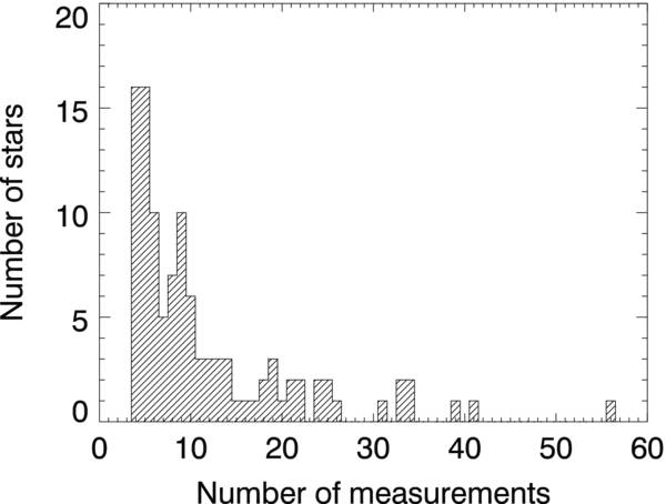
Figure 1. Distribution of number of Doppler measurements per star for those M2K stars selected for the analysis of giant planet fraction. One star (HIP 57274) with two giant planets has 120 observations and is off scale.
Download figure:
Standard image High-resolution imageIdeally, we would have defined our sample of late K dwarfs in terms of effective temperature Teff, a fundamental stellar parameter, but not all our stars have spectroscopically-determined values. Thus, we selected stars based on V − J color as a proxy for Teff. We restricted the sample to 140 stars with 1.8 < V − J < 2.8, corresponding to 3900 < Teff < 4750 K or spectral subtypes K3–K7 (Gray & Corbally 2009), based on an empirical color–Teff relation using stars with measured angular diameters (Boyajian et al. 2012). We corroborated this selection by estimating the Teff of many of these stars using spectra (Figure 2). Stellar parameters (including Teff and metallicity [Fe/H]) of stars with 1.8 < V − J < 2.3 were estimated using the Spectroscopy Made Easy (SME) package (Valenti & Piskunov 1996; Table 2). SME performs poorly on dwarfs with V − J > 2.3 and Teff ⩽ 4300 K so for these stars we estimated Teff by comparing moderate-resolution (R ∼ 1500) visible-wavelength (3500–8500 Å) spectra obtained with the Supernova Integral Field Spectrograph (Lantz et al. 2004) on the University of Hawaii 2.2 m telescope with synthetic spectra generated by the PHOENIX BT-SETTL program (Allard et al. 2011). The comparison procedure is described in Lépine et al. (2013) and was adjusted (A. W. Mann et al. 2013, in preparation) to maximize agreement with the calibrator stars of Boyajian et al. (2012). For stars without spectra, we estimated Teff using V − J color and the Boyajian et al. (2012) relation (Table 2).
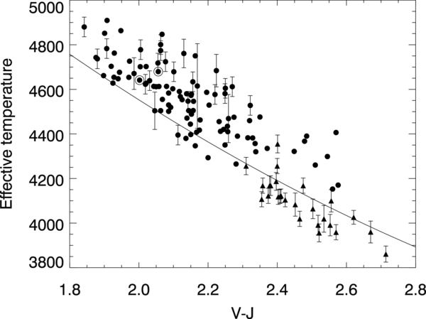
Figure 2. Stellar effective temperature vs. V − J color of late K dwarfs in the M2K Doppler survey. Circles represent temperatures from SME analyses of high-resolution spectra (Valenti & Piskunov 1996), whereas triangles represent temperatures from fitting medium-resolution spectra to PHOENIX synthetic spectra (A. W. Mann et al. 2013, in preparation) and calibrating on stars in Boyajian et al. (2012). Only some error bars are shown for clarity. The solid curve is an empirical Teff vs. V − J relation from Boyajian et al. (2012). Two systems with published giant planets (HIP 57274 and HIP 2247) are circled.
Download figure:
Standard image High-resolution imageTable 2. Stars Included in the Analysis
| Name | V − J | Teff (K) | (Fe/H) | S | M (M☉) | Nobs | rms (m s−1) | p1 |
|---|---|---|---|---|---|---|---|---|
| HIP 1078 | 2.13 | 4426b | ⋅⋅⋅ | 0.49 | 0.75 | 4 | 2.56 | 0.005 |
| HIP 1532 | 2.52 | 3956a | −0.37 | 0.84 | 0.64 | 24 | 4.28 | 0.011 |
| HIP 2247 | 2.06 | 4680 | 0.24 | 0.62 | 0.77 | 12 | 0.00 | 0.000 |
| HIP 3418 | 2.16 | 4546 | 0.02 | 0.50 | 0.73 | 5 | 1.54 | 0.004 |
| HIP 4353 | 2.20 | 4587 | 0.17 | 0.70 | 0.77 | 6 | 12.89 | 0.961 |
| HIP 4454 | 1.99 | 4671 | −0.55 | 0.35 | 0.71 | 5 | 3.62 | 0.004 |
| HIP 4845 | 2.58 | 4170 | −0.19 | 1.67 | 0.63 | 33 | 3.55 | 0.005 |
| HIP 5247 | 2.51 | 4260 | −0.22 | 0.63 | 0.66 | 12 | 7.76 | 0.052 |
| HIP 5663 | 2.34 | 4357 | −0.05 | 1.04 | 0.68 | 24 | 0.00 | 0.000 |
| HIP 6344 | 2.32 | 4383 | −0.04 | 0.99 | 0.68 | 5 | 1.71 | 0.007 |
| HIP 9788 | 2.15 | 4444 | −0.37 | 0.73 | 0.67 | 17 | 4.53 | 0.008 |
| HIP 10337 | 2.54 | 4019a | 0.12 | 1.58 | 0.66 | 22 | 7.74 | 0.019 |
| HIP 10416 | 1.88 | 4743 | 0.14 | 0.71 | 0.76 | 11 | 10.43 | 0.721 |
| HIP 11000 | 1.92 | 4703 | 0.20 | 0.76 | 0.73 | 13 | 10.54 | 0.195 |
| HIP 12493 | 2.25 | 4350 | −0.29 | 0.66 | 0.68 | 6 | 4.50 | 0.032 |
| HIP 13375 | 2.50 | 4110b | 0.00 | 0.59 | 0.56 | 9 | 3.68 | 0.010 |
| HIP 14729 | 2.15 | 4579 | 0.17 | 1.00 | 0.70 | 10 | 5.76c | 0.007 |
| HIP 15095 | 2.28 | 4265 | −0.21 | 1.28 | 0.68 | 10 | 6.82 | 0.071 |
| HIP 15563 | 2.06 | 4718 | 0.16 | 1.04 | 0.72 | 12 | 10.74 | 0.332 |
| HIP 15673 | 1.93 | 4654 | −0.46 | 0.50 | 0.69 | 6 | 3.12 | 0.007 |
| TYC 1234-00069-1 | 1.90 | 4522a | ⋅⋅⋅ | 0.42 | 0.75 | 4 | 1.30 | 0.023 |
| HIP 17346 | 2.06 | 4613 | 0.07 | 0.59 | 0.74 | 6 | 4.19 | 0.012 |
| HIP 17496 | 2.15 | 4489 | −0.04 | 0.62 | 0.72 | 5 | 2.53 | 0.008 |
| HIP 19165 | 2.24 | 4412 | −0.22 | 0.64 | 0.65 | 31 | 5.16 | 0.010 |
| HIP 19981 | 2.25 | 4605 | 0.27 | 0.70 | 0.77 | 5 | 4.60 | 0.017 |
| HIP 20359 | 2.14 | 4547 | −0.04 | 0.58 | 0.75 | 5 | 4.47 | 0.011 |
| HIP 25220 | 2.04 | 4613 | 0.05 | 0.89 | 0.71 | 10 | 7.92 | 0.049 |
| HIP 26196 | 2.34 | 4245b | ⋅⋅⋅ | 0.76 | 0.74 | 8 | 4.26d | 0.012 |
| TYC 4356-01014-1 | 1.88 | 4737 | −0.17 | 0.46 | 0.77 | 8 | 2.69 | 0.003 |
| HIP 29548 | 2.32 | 4528 | −0.10 | 0.59 | 0.69 | 20 | 3.79 | 0.006 |
| HIP 30112 | 2.36 | 4168a | ⋅⋅⋅ | 1.46 | 0.72 | 25 | 7.45 | 0.040 |
| HIP 30979 | 2.02 | 4627 | 0.23 | 0.60 | 0.77 | 12 | 5.41 | 0.005 |
| TYC 3388-01009-1 | 2.36 | 4220b | ⋅⋅⋅ | 1.38 | 0.68 | 10 | 64.66 | 0.500 |
| HIP 32769 | 2.24 | 4420 | −0.05 | 0.68 | 0.71 | 16 | 4.86 | 0.005 |
| HIP 32919 | 2.33 | 4382 | −0.01 | 0.86 | 0.70 | 18 | 5.29 | 0.006 |
| TYC 1352-01588-1 | 2.31 | 4270b | ⋅⋅⋅ | 0.00 | 0.69 | 7 | 18.27 | 0.918 |
| TYC 0748-01711-1 | 2.50 | 4064a | ⋅⋅⋅ | 0.16 | 0.66 | 25 | 42.28c | 0.500 |
| HIP 36551 | 2.09 | 4501 | −0.30 | 0.57 | 0.70 | 11 | 3.86 | 0.007 |
| HIP 37798 | 2.54 | 4082b | ⋅⋅⋅ | 1.42 | 0.70 | 9 | 3.12 | 0.005 |
| HIP 38969 | 2.13 | 4761 | 0.26 | 0.40 | 0.81 | 10 | 10.96c | 0.817 |
| HIP 40375 | 2.18 | 4463 | 0.03 | 0.96 | 0.71 | 33 | 6.67 | 0.009 |
| HIP 40671 | 2.05 | 4612 | 0.06 | 0.46 | 0.74 | 6 | 1.95 | 0.008 |
| HIP 40910 | 2.41 | 4119a | −0.06 | 1.41 | 0.68 | 21 | 9.47 | 0.665 |
| HIP 41130 | 2.26 | 4410 | −0.10 | 1.10 | 0.72 | 18 | 8.46 | 0.603 |
| HIP 41443 | 2.08 | 4613 | 0.01 | 0.83 | 0.74 | 9 | 6.10 | 0.014 |
| HIP 42567 | 1.94 | 4648 | 0.09 | 0.71 | 0.76 | 6 | 6.00 | 0.037 |
| HIP 43534 | 2.56 | 4100a | −0.13 | 1.49 | 0.64 | 14 | 6.88 | 0.006 |
| HIP 43667 | 2.12 | 4554 | 0.01 | 0.51 | 0.72 | 9 | 5.24 | 0.020 |
| HIP 44072 | 2.16 | 4347 | −0.42 | 0.52 | 0.71 | 5 | 3.96 | 0.020 |
| HIP 45042 | 2.35 | 4476 | 0.17 | 1.27 | 0.73 | 5 | 9.94 | 0.095 |
| TYC 1955-00658-1 | 2.52 | 3991a | 0.21 | 1.48 | 0.66 | 4 | 6.05 | 0.055 |
| HIP 45839 | 2.12 | 4590 | 0.05 | 0.55 | 0.72 | 5 | 12.40 | 0.865 |
| HIP 46343 | 2.20 | 4529 | 0.03 | 1.03 | 0.70 | 10 | 4.35 | 0.008 |
| HIP 46417 | 2.28 | 4475 | −0.06 | 0.69 | 0.71 | 9 | 7.19 | 0.018 |
| HIP 47201 | 2.37 | 4122a | 0.03 | 0.98 | 0.69 | 7 | 4.91 | 0.045 |
| HIP 48139 | 2.09 | 4548a | 0.22 | 0.45 | 0.77 | 6 | 2.34 | 0.004 |
| HIP 48411 | 2.14 | 4505 | 0.20 | 0.78 | 0.73 | 4 | 8.32 | 0.057 |
| HIP 48740 | 2.22 | 4577 | 0.02 | 1.10 | 0.72 | 8 | 7.38 | 0.015 |
| HIP 50960 | 2.40 | 4187a | −0.06 | 1.51 | 0.65 | 8 | 8.22 | 0.023 |
| HIP 51443 | 2.16 | 4505 | −0.05 | 1.09 | 0.71 | 19 | 8.56 | 0.447 |
| HIP 53327 | 2.29 | 4390 | −0.79 | 0.37 | 0.66 | 4 | 5.13 | 0.018 |
| HIP 54459 | 2.26 | 4469 | −0.52 | 0.37 | 0.68 | 13 | 8.32 | 0.028 |
| HIP 54651 | 2.11 | 4395 | −0.89 | 0.33 | 0.66 | 6 | 1.63 | 0.002 |
| HIP 54810 | 2.09 | 4256a | 0.03 | 1.04 | 0.70 | 5 | 6.18 | 0.061 |
| HIP 55507 | 2.42 | 4104a | −0.05 | 0.90 | 0.69 | 22 | 6.37c | 0.013 |
| HIP 56630 | 2.67 | 3960a | −0.01 | 1.37 | 0.68 | 9 | 7.29 | 0.045 |
| HIP 57274 | 2.00 | 4641 | 0.08 | 0.39 | 0.76 | 120 | 0.00 | 1.000 |
| HIP 57493 | 2.38 | 4168a | 0.06 | 1.16 | 0.71 | 15 | 5.48 | 0.009 |
| HIP 59496 | 2.41 | 4122a | −0.01 | 1.42 | 0.69 | 7 | 9.67 | 0.203 |
| HIP 60633 | 2.08 | 4724 | 0.25 | 0.33 | 0.76 | 26 | 12.92 | 1.000 |
| HIP 62406 | 2.38 | 4168a | 0.31 | 1.10 | 0.68 | 39 | 8.07 | 0.118 |
| HIP 62847 | 1.97 | 4726 | 0.05 | 0.66 | 0.81 | 34 | 6.03 | 0.012 |
| HIP 63894 | 2.20 | 4361b | ⋅⋅⋅ | 0.81 | 0.69 | 8 | 6.47 | 0.029 |
| HIP 64048 | 2.17 | 4615 | 0.08 | 0.71 | 0.71 | 14 | 8.63 | 0.029 |
| HIP 64262 | 2.03 | 4639 | −0.25 | 0.59 | 0.70 | 9 | 8.13 | 0.047 |
| HIP 66074 | 2.32 | 4460 | 0.23 | 1.17 | 0.73 | 9 | 11.06 | 0.818 |
| HIP 66222 | 2.71 | 3861a | −0.11 | 1.34 | 0.68 | 13 | 6.54 | 0.017 |
| HIP 66283 | 1.84 | 4880 | 0.18 | 0.00 | 0.84 | 7 | 10.71 | 0.256 |
| HIP 66840 | 2.47 | 4019a | ⋅⋅⋅ | 0.00 | 0.69 | 5 | 1.96 | 0.008 |
| HIP 67842 | 2.76 | 3919b | ⋅⋅⋅ | 1.23 | 0.64 | 6 | 5.18 | 0.016 |
| HIP 73427 | 2.40 | 4256a | −0.02 | 1.26 | 0.73 | 11 | 13.32 | 0.949 |
| HIP 75672 | 2.45 | 4083a | ⋅⋅⋅ | 0.00 | 0.69 | 4 | 2.67 | 0.021 |
| HIP 77908 | 2.27 | 4612 | 0.28 | 0.98 | 0.74 | 5 | 2.50 | 0.008 |
| HIP 78184 | 2.47 | 4168a | ⋅⋅⋅ | 0.00 | 0.68 | 4 | 7.08 | 0.004 |
| HIP 78999 | 2.05 | 4504 | 0.24 | 0.00 | 0.73 | 4 | 6.30 | 0.029 |
| HIP 79698 | 2.31 | 4256a | 0.26 | 0.91 | 0.74 | 7 | 3.51 | 0.004 |
| HIP 87464 | 2.17 | 4417 | −0.27 | 0.44 | 0.69 | 8 | 8.76 | 0.351 |
| HIP 89087 | 2.40 | 4118a | −0.01 | 1.38 | 0.68 | 4 | 3.48 | 0.001 |
| HIP 93871 | 2.06 | 4453a | −0.47 | 0.28 | 0.71 | 4 | 3.38 | 0.001 |
| HIP 97051 | 2.34 | 4320 | −0.19 | 1.10 | 0.62 | 19 | 9.10 | 0.183 |
| HIP 99205 | 2.15 | 4397 | −0.18 | 0.85 | 0.64 | 6 | 6.32 | 0.021 |
| HIP 99332 | 2.15 | 4400a | 0.30 | 0.73 | 0.76 | 8 | 5.82 | 0.033 |
| HIP 101262 | 2.06 | 4774 | 0.19 | 1.00 | 0.73 | 4 | 9.06 | 0.146 |
| HIP 102332 | 2.39 | 4202b | ⋅⋅⋅ | 0.75 | 0.66 | 4 | 5.56 | 0.017 |
| HIP 103650 | 2.10 | 4603 | −0.04 | 0.75 | 0.71 | 9 | 5.22 | 0.020 |
| HIP 104092 | 2.23 | 4455 | 0.07 | 0.54 | 0.72 | 5 | 6.66 | 0.057 |
| HIP 105341 | 2.55 | 4299 | −0.05 | 1.38 | 0.68 | 5 | 8.68 | 0.087 |
| HIP 109980 | 2.14 | 4580 | 0.00 | 0.95 | 0.71 | 56 | 6.73 | 0.024 |
| HIP 110774 | 2.14 | 4471 | −0.12 | 0.87 | 0.67 | 4 | 1.91 | 0.000 |
| TYC 3995-01436-1 | 2.16 | 4634 | 0.08 | 0.89 | 0.71 | 9 | 7.20 | 0.051 |
| HIP 112496 | 2.00 | 4778 | 0.04 | 0.65 | 0.75 | 5 | 7.92 | 0.059 |
| HIP 112918 | 2.26 | 4434 | 0.02 | 1.20 | 0.67 | 4 | 2.80 | 0.018 |
| HIP 114156 | 2.45 | 4322 | −0.02 | 1.43 | 0.66 | 4 | 3.41 | 0.025 |
| HIP 115004 | 2.22 | 4684 | −0.11 | 0.83 | 0.82 | 21 | 40.79c | 0.500 |
| HIP 117197 | 2.56 | 4153 | −0.38 | 1.05 | 0.61 | 19 | 3.15 | 0.002 |
| HIP 117492 | 2.10 | 4679 | 0.08 | 0.98 | 0.73 | 5 | 5.09 | 0.029 |
| HIP 117559 | 2.25 | 4581 | 0.07 | 1.28 | 0.71 | 41 | 9.82 | 0.447 |
| HIP 117946 | 1.95 | 4863 | 0.03 | 0.85 | 0.77 | 14 | 9.00 | 0.143 |
| HIP 118261 | 1.90 | 4662 | −0.04 | 0.65 | 0.74 | 34 | 7.28 | 0.025 |
| HIP 118310 | 2.24 | 4326b | ⋅⋅⋅ | 0.71 | 0.80 | 4 | 0.00 | 0.000 |
Notes. aBased on medium-resolution spectroscopy. bBased on V − J color. cA linear trend removed. dA parabolic trend removed.
The median offset between SME-derived and V − J-based temperatures is 140 K. For this reason, we included the 13 stars with SME-based Teff > 4750 K (but acceptable V − J) as their actual effective temperatures are probably within the acceptable range. Unsurprisingly, Teff estimates based on calibrated comparisons between moderate-resolution spectra and PHOENIX models are consistent with the Boyajian et al. (2012) relation. Nearly all of our stars have measured parallaxes and we estimated masses using the relation with absolute K magnitude in Henry & McCarthy (1993). For those few stars lacking parallaxes we used the empirical relations between Teff, stellar radius, and stellar mass in Boyajian et al. (2012).
We excluded stars exhibiting relatively high emission in the H and K lines of Ca ii. These stars are chromospherically active and tend to exhibit higher astrophysical Doppler noise or "jitter" (e.g., Isaacson & Fischer 2010). Figure 3 shows values of SHK, the flux in the Ca ii line cores normalized by the continuum, versus V − J color. The trend of increasing SHK with redder V − J is due to the lower blue continuum rather than elevated Ca ii emission in redder stars. We calculated a running median (N = 20), fit a linear function  with V − J, and subtracted that from these values. The histogram (inset of Figure 3) suggests a cutoff at
  , which rejects 11 stars as exceptionally active. Among the stars we admitted were five for which it was not possible to estimate SHK because the continuum was not detected.
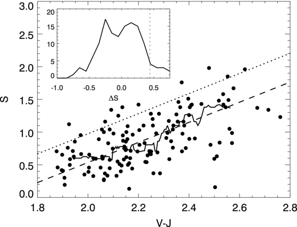
Figure 3. Flux S in the core of the Ca ii HK lines, normalized by the continuum, vs. V − J color. High values of S are associated with elevated stellar activity and astrophysical Doppler noise or "jitter." The solid line is a running median (N = 20), the dashed line is a linear regression of the median  , and the dotted line is the linear fit + 0.44, above which stars were excluded from the analysis. This threshold was selected based on the distribution of
  (inset). Eleven stars or 8% of the sample were excluded based on this criterion.
Download figure:
Standard image High-resolution imageWe next considered the distribution of RV standard deviations (rms) of the remaining 129 stars. The majority (100) of the stars fall in a cluster with rms <15 m s−1 (Figure 4). We inspected the RV data of the 29 stars with rms >15 m s−1. One of these is HIP 57274, which has been described elsewhere (Fischer et al. 2012). Eight others have additional stars within 5 arcsec and were excluded because leakage of light into the spectrograph slit is an established source of RV error.

Figure 4. Distribution of adjusted radial velocity rms among 110 M2K stars after excluding or adjusting case of high rms. One star with rms = 65 m s−1 falls outside the plot. Systems with rms >15 m s−1 were either excluded or significant linear/quadratic trends fitted and removed (see the text). The solid curve is the best-fit model for the resulting distribution at rms <15 m s−1 assuming pure Gaussian-distributed noise that is the sum of formal errors and an astrophysical noise term σ0 that includes both stellar jitter and barycenter motion due to small planets. The value σ0 = 6.3 m s−1 which best reproduces the observed distribution was selected by maximizing the Kolmogorov–Smirnov statistic that the actual and model rms values are drawn from the same distribution (inset).
Download figure:
Standard image High-resolution imageWe analyzed each of the remaining 20 sets of RVs with both weighted linear and quadratic regressions and applied an F-test to evaluate the significance of any reduction in variation after subtraction of the fit. Although all stars have ⩾4 RV measurements, and thus the number of degrees of freedom for a quadratic fit is ⩾1, irregular sampling means that overfitting and erroneous reduction in RV variation is possible. For example, four observations in two very closely spaced pairs cannot be reliably regressed: a significant RV offset between the pairs could be the result of a linear trend or any RV variation. To identify such cases, we computed an effective N equal to the sum of normalized Voronoi-type weights wi = (ti + 1 − ti − 1)/2 that are often assigned by regularization algorithms (Strohmer 2000). End points have weights w1 = t2 − t1 and wN = tN − tn − 1. Thus,
In the limit of large N, the effective number of points Neff and thus the maximum order of the polynomial that should be used in a regression approach the total time interval divided by the maximum interval between points. This is analogous to the Nyquist sampling criterion.
Doppler data sets with rms >15 m s−1 were processed in one of three ways: (1) if regressions did not significantly reduce variance (F-test; p < 0.05), the data were analyzed as is. (2) If a regression did significantly reduce variance and Neff was >3 (or >4, in the case of a quadratic), the best fit is subtracted before analysis. (3) If a regression is significant but Neff is not sufficiently large, the star and its data were excluded from the analysis. We excluded 11 stars in this way, leaving 110 stars for analysis, including HIP 57274.
HIP 2247 has a long-period super-Jupiter previously identified by Moutou et al. (2009). We fit the combined HARPS and Keck-HIRES data using the RVLIN code (Wright & Howard 2009), generating errors using 100 Monte Carlo realizations of the data by randomly reshuffling the residuals to the previous fit. We find essentially the same planetary parameters as Moutou et al. (2009), but with significantly reduced uncertainties: Mpsin i = 5.14 ± 0.02 MJ, P = 655.90 ± 0.22 days, and e = 0.543 ± 0.0011, with a residual rms of 3.8 m s−1 (Figure 5). No significant trend was found (−0.0024 ± 0.0011 m s−1). The uncertainty in msin i does not include errors in the estimated stellar mass of 0.77 M☉. Any giant planets with P < 245 days can be ruled out: we include this system in our sample but consider it a definitive non-detection.
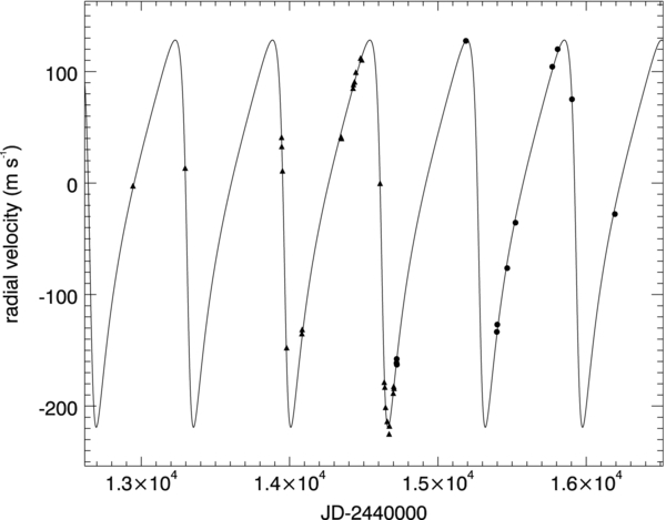
Figure 5. Thirty-eight radial velocities of HIP 2247 showing barycenter motion produced by the long-period giant planet discovered by Moutou et al. (2009). Triangles are Moutou et al. measurements with HARPS and circles are M2K measurements with Keck-HIRES. The solid line is the best-fit Keplerian orbit with msin i = 5.14 MJ, PK = 655.9 days, and e = 0.543.
Download figure:
Standard image High-resolution imageHIP 38117 exhibits RV variation consistent with the presence of a stellar-mass companion on a 81.28 ± 0.01 day orbit with an eccentricity of 0.478 ± 0.012 (Figure 6). Assuming a primary mass of 0.73 M☉ based on the system's V − J color, and assuming that the secondary contributes negligible flux, the companion's M*sin i is 0.45 ± 0.16 M☉, i.e., this is a very late K or M dwarf. (This calculation assumes an average value of 〈sin i〉 = π/4 to calculate the total system mass.) The residual rms is 3 m s−1 (N = 15). As a planetary orbit with a comparable orbital period is unlikely to be stable, we follow the suit of other studies by excluding this binary system from our analysis.

Figure 6. Fifteen M2K radial velocities of the K+M binary star system HIP 38117. The best-fit Keplerian orbit has PK = 81.28 days and e = 0.478.
Download figure:
Standard image High-resolution image2.2. Estimation of Planet Fraction
We estimated the fraction of stars f with giant planets having MP > 0.3MJ (i.e., Saturn mass) and Keplerian orbital periods 1.7 days <PK < 245 days. The choice of outer cutoff in PK is based on the temporal baseline of our data—nearly all stars were monitored for at least 245 days—and motivated by the longest bin with good statistics in the analysis of Kepler planet candidates by Fressin et al. (2013). The inner cutoff corresponds to the location of the rollover in the period distribution of giant planets around Kepler stars (Howard et al. 2012). We construct and maximize a likelihood function to find the most probable value of f and its uncertainty. The details of the calculations are given in the Appendix and the method is only summarized here.
A standard procedure to estimate the fraction of stars with planets is to maximize a binomial expression involving the product of detections and non-detections. However, with RV data it can be difficult or impossible to rule out all possible planets, e.g., those on face-on orbits. Thus, we replace detections and non-detections with a Bayesian statistic that is sum of the probabilities  and
and  that there are zero or one giant planets around the ith star, with 1 − f and f as priors for zero or one planets, respectively,
where the sum is over all stars. This counts multi-giant planet systems once, and thus underestimates the planet occurrence
(planets per star). The probabilities  and
and  are Gaussian functions of the difference between the predicted and observed RVs vij and
  , weighted by priors
  marginalized over all model parameters
and where σij are the formal errors, astrophysical noise or "jitter," as well as systematic error and the contribution of small planets to motion of the star around the system's barycenter (see Section 4.1), added in quadrature. This method is analogous to the approach used in Gaidos et al. (2012) but uses the individual RV measurements, not the rms.
The Gaussian form of Equation (3) means that only the best-fit sets of parameter values (barycenter motion v0, Keplerian period PK, Doppler amplitude K, eccentricity e, longitude of periastron ω, and time of periastron t0) make significant contributions to p0 or p1. We used the linear dependence of the RVs on the barycenter velocity v0 and Doppler amplitude K to analytically solve for the best-fit values of these two parameters given values for the other parameters. To marginalize over planet mass we used the relation between K, planet mass, and orbital inclination and adopt a power-law distribution of log mass with an index α = −0.31 (Cumming et al. 2008). (The sensitivity of our results to this value is explored in Section 4.2.) We marginalized Equation (3) over the full range of possible values of e, ω, t0, using a Rayleigh function for the prior on eccentricity (Moorhead et al. 2011) and uniform priors for ω and t0. We further evaluated the probability over 1.7 < PK < 245 days at intervals of equal prior probability, assuming a power-law distribution for log period having index β = 0.26 (Cumming et al. 2008). To better sample intervals of PK corresponding to higher probability we used each PK value as an initial value in a fit of a Keplerian solution to the data with the RVLIN routine (Wright & Howard 2009). We used the fixed, best-fit values of the other parameters for the RVLIN fit, obtained an adjusted value of PK, and then re-calculated the other parameters as described above. This procedure was repeated twice, which we found was sufficient for convergence.
We calculated p0 and p1 by summing over final values of all the parameters, and normalizing by p0 + p1. For three stars, p0 and p1 were both incalculably small due to large disagreements between v and  for either the zero- or one-planet models. This could be due to elevated stellar jitter or the presence of smaller planets (see below). For these stars we assigned p0 = p1 = 0.5, i.e., the zero- and one-planet models are accepted or rejected with equal likelihood. We then evaluated Equation (2) over all possible values of f, and found the maximum. We calculated an approximate uncertainty by assuming asymptotic normality, iteratively fitting a parabola to the log-likelihood curve, and assigning
  , where C is the curvature coefficient of the parabola.
Both the zero- and one-planet models do not account for barycenter motion due to the presence of other, smaller planets, as well as any sources of systematic error. As a result, for some stars both models are strongly rejected, leading to an erroneously high value of f. To account for this effect, we treat this barycenter motion as an additional source of uncorrelated, random RV noise or "jitter" that, along with stellar noise, can be described by a single value of σ0. A value for σ0 was chosen by assuming that the pronounced cluster of systems with rms <15 m s−1 (Figure 4) represents stars without giant planets, and fitting that distribution by a Monte Carlo model. We constructed 1000 artificial realizations of the data with the same number of RVs per star but drawn from a random normal distribution. The variance of this distribution was set equal to the formal measurement error and a trial value of σ0 added in quadrature. We computed the rms values and comparing the distribution to the observed distribution (after subtracting any trends) with a two-sided Kolmogorov–Smirnov (K-S) test. We found that a curve with σ0 = 6.3 m s−1 (solid curve in Figure 4) maximizes the K-S probability of the Monte Carlo distribution (inset of Figure 4), and we use that value in our estimation of f. The poor agreement between the observed and "best-fit" distributions reflects the inability of a single value of σ0 to capture the diversity of stellar RV behavior.
3. METHODS: KEPLER SURVEY
We compared our estimate of the fraction of M2K dwarfs with giant planets with one for late K dwarfs observed by Kepler. We selected Kepler targets with 1.8 < V − J < 2.8, with V magnitudes estimated using the relation V = r + 0.44(g − r) − 0.02 (Fukugita et al. 1996). We further limited the sample to stars that had been observed in at least seven of quarters Q1–Q8. The absence of a single quarter will minimally affect the detection efficiency but is common because some stars were added after Q1 and others fall within Kepler's defunct CCD module during one of four rotations of the spacecraft. Stellar and planetary parameters of Kepler stars were estimated by fits to Dartmouth stellar models (Dotter et al. 2008) using the Bayesian procedure described in Gaidos (2013). We restricted the analysis to 6293 dwarf stars with 3900 < Teff < 4800 K, log g > 4, and KP < 16. In this sample are two giant planet candidates with PK < 245 days: KOI 1176.01 is a hot Jupiter (PK = 1.94 days) orbiting a star with Teff ≈ 4625 K. The second (KOI 868.01) has an orbital period of 235.9 days. Another giant planet candidate (KOI 1466.01) has PK = 281.6 days and was excluded, and a fourth (KOI 1552.01) was excluded from our sample because Kepler observed it for only five of the eight quarters.
Following Mann et al. (2012), we calculated the binomial log likelihood for a flat log distribution with period and a monotonic radius distribution in the limit that the transit probability is low:
where the orbital period range is P1 < PK < P2, the two summations are over detections and non-detections, respectively, Di(P) is the probability of detecting a planet around the ith star,
and an uninteresting constant is ignored. To compare with the M2K results, we use P1 = 1.7 days and P2 = 245 days.
We assumed that any transit of a giant planet in front of a late K dwarf will be detected. The typical transit depth is ∼0.02, which is far larger than the noise: the median 3 hr combined differential photometry precision for these stars is 1.8 × 10⁻⁴ and the 99% value is 6.6 × 10⁻⁴, corresponding to S/N of ∼110 and 30, respectively. Fressin et al. (2013) found that the recovery rate of the Kepler detection pipeline was nearly 100% for S/N > 16. Thus, the detection probability is simply the geometric factor R*/a, where a is the orbital semimajor axis, and
We marginalized F (Equation (5)) over e and ω and adopted a distribution n(e) for eccentricity. Ignoring terms that do not depend on f, Equation (4) becomes
where ND is the number of detected planets and ρ is the mean density of the star. Adopting the function for n(e) in Shen & Turner (2008), we found that the integral is only weakly dependent on the parameter a in their distribution, and is ≈1.20 for a = 4. Using a Rayleigh distribution like that for the M2K analysis gives a similar value (1.08) for the integral. Because each star can be explained by more than one stellar model with probability p, we used a weighted mean of ρ−1/3 to calculate the likelihood:
where the summation is restricted to main-sequence models, i.e., log g > 4.
We compared our analysis with that of Howard et al. (2012) by calculating f for dwarfs with 4100 < Teff < 4600 K and 4600 < Teff < 5100 K, and restricting the period range to 0.68 days <PK < 50 days. Our results are 0% and 0.3% for the respective Teff bins, compared to 0% and  % from Howard et al. (2012). Despite the same restrictions on Teff, there are differences in the samples because we reclassified some K stars as giants (and any candidate giant planets as stellar companions) and we imposed a V − J color cut which excludes many systems from the hotter Teff bin, whereas Howard et al. (2012) required KP < 15.
4. RESULTS AND DISCUSSION
4.1. Fraction of Stars with Giant Planets
Values of p1, the probability that the RV data are consistent with the presence of a giant planet with PK < 245 days, are reported for the 110 late K dwarfs in Table 2 (note that p0 = 1 − p1). Figure 7 shows the relative likelihood distribution of f constructed from these values using Equation (2). The most probable value of f is 4.0% and the uncertainty based on the assumption of asymptotic normality is ±2.3%. The elevated range relative to the rate of actual detections (1 of 110 stars) is due to the presence of several stars in our sample with significantly non-zero values of p1. Eighteen stars have p1 > 0.2 and four, excluding HIP 57274, have p1 > 0.9 (Table 2). We are continuing to monitor these stars (T. S. Boyajian et al. 2013, in preparation). If we assume that giant planets with PK < 245 days are ruled out (p1 = 0) for all stars other than HIP 57274 (the "HIP 57274 only" case in Figure 7), the most probable value of f becomes 0.92% ± 0.75%.
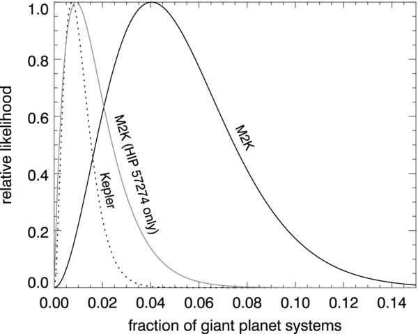
Figure 7. Probability distribution of the fraction of 110 M2K stars with giant planets with Mp > 0.3MJ and PK < 245 days (solid curves). The curve labeled "HIP 57274 only" assumes that such planets are ruled out around all but one of the stars: HIP 57274. The dashed line is the probability distribution of the fraction of Kepler late K dwarfs having giant planets with 0.7RJ < Rp < 2RJ and PK < 245 days.
Download figure:
Standard image High-resolution imageStars may exhibit high RV variation for reasons other than the presence of giant planets with P < 245 days. Many M2K target stars were monitored for intervals ≫245 days and our RV data are sensitive to the presence of planets on wider orbits. Both Doppler and Kepler surveys find such planets, e.g., HIP 2247 and KOI 1466.01 (see below). Some stars may have a lower-mass (M dwarf) companion like that of HIP 38117 (Figure 6), but on a wider orbit. If the trend in RV produced by such a companion is not resolved because of undersampling, it will manifest itself as a high rms. Despite our precautionary elimination of stars with Ca ii HK emission, some stars in our sample may have high intrinsic "jitter" from spots. Many stars in our sample have only a few Doppler observations (Figure 1), confounding these effects. Ultimately, additional observations are required to discriminate between these possibilities.
The relative likelihood distribution of f for late K dwarfs observed by Kepler is plotted as the dashed line in Figure 7. The most likely value of f is 0.7% ± 0.5%. Based on the two distributions, we calculate a 99% probability that the Kepler value is actually lower than the M2K value. Due to the factors discussed above, the M2K value of 4% may be an overestimate: There is a closer correspondence (85% chance that the Kepler estimate is lower) if we rule out giant planets around all stars other than HIP 57274. Wright et al. (2012) report that the occurrence of "hot" Jupiters around the FGK stars in the CPS Doppler survey is 1.2%, compared to 0.4% for Kepler (Howard et al. 2012; Fressin et al. 2013). Gaidos & Mann (2013) proposed that the difference between the transit and Doppler results may be due to the presence of subgiants in the Kepler target catalog: planets around such stars will be more difficult to detect and more likely to experience destructive orbital decay. This explanation may be less applicable to late K spectral types where the giant and main-sequence branches are more distinguishable, and we consider orbits with PK ≫ 10 days on which orbital decay will be negligible. Another explanation for at least some of this difference is that the exclusion of spectroscopic and resolved binaries from the M2K sample, but not the Kepler sample, may enrich for giant planets, presuming that such binaries are less likely to host planets for dynamical reasons (e.g., Thébault et al. 2006; Bonavita & Desidera 2007; Kaib et al. 2013).
We compare our M2K and Kepler estimates of f for late K dwarfs with previous studies for different ranges of stellar mass (Figure 8). Our estimates bridge the gap between solar-type stars (Fischer & Valenti 2005; Cumming et al. 2008; Johnson et al. 2010; Howard et al. 2010, 2012; Fressin et al. 2013) and M dwarfs (Naef et al. 2005; Cumming et al. 2008; Johnson et al. 2010; Bonfils et al. 2013; Fressin et al. 2013). We have adjusted values by the factor  to account for differences in the maximum orbital period Pmax of each survey, assuming a flat distribution with ln PK. (The adjustment is not sensitive to the exact distribution assumed.) The surveys also differ somewhat in the mass or radius ranges of objects counted as giant planets. For example, although our Kepler-based estimate of 0.7% for late K dwarfs seems much lower than those of Fressin et al. (2013) for either GK dwarfs (6.1% ± 0.9%) or M dwarfs (3.6% ± 1.7%), these statistics are for PK < 418 days rather than 245 days, and Rp > 6 R⊕, rather than the 8 R⊕ convention adopted here. Their overall f falls to 4.1% for P < 245 days, and our f rises to 1.1% ± 0.6% if we include planets with Rp > 6 R⊕, bringing these two figures closer. Taken together, these estimates suggest an overall trend, perhaps linear, of increasing giant planet occurrence with stellar mass, there is not yet any indication of finer structure. A linear least-squares fit to the adjusted Doppler data yields f(%) = −1.11 + 5.33 M*/M☉ (dashed line in Figure 8) with weak significance (F-test probability of 0.12). This compilation also suggests that the deficit of giant planets around Kepler stars relative to the targets of Doppler surveys (Wright et al. 2012) depends on host star mass (Figure 8), although clearly a more homogeneous analysis of the collective data sets is needed.

Figure 8. Adjusted percentage of stars with giant planets (Saturn mass or greater) vs. stellar mass. Points are color-coded according to their source and the symbol indicates whether the estimate is based on an RV (triangles) or transit (circles) survey. Each estimate was adjusted by the factor  to account for different choices of maximum orbital period Pmax (see the legend). The unadjusted values are plotted as smaller open symbols of the same type and color. The range of stellar masses is in some cases approximate. The dashed line is a linear least-squares fit to the adjusted Doppler estimates.
Download figure:
Standard image High-resolution image
A correlation between giant planets and the metallicity of the host star has been unambiguously established for solar-type stars (e.g., Fischer & Valenti 2005), and is strongly supported by the available evidence for M dwarfs (Neves et al. 2013; Mann et al. 2013). The median metallicity of our sample of late K dwarfs is solar ([Fe/H] = 0.004). The metallicities of HIP 57274 and HIP 2247, the two stars known to host giant planets in our sample, are 0.08 and 0.24 dex, consistent with this trend. The difference in the distributions of metallicities of stars with p1 < 0.1 (median [Fe/H] of −0.01) and those with p1 > 0.1 (median [Fe/H] of 0.08) is marginally significant (K-S probability of 0.06), further supporting a giant planet–metallicity relation in late K dwarfs. If SME overestimates the Teff of these stars (Figure 2), the [Fe/H] is also overestimated by about 0.1 dex per 100 K.
4.2. Sensitivity to Parameter Values
Our estimates of f may be sensitive to the values of any one of several parameters we use in our calculations (see the Appendix). These include the computational resolution n with which  is evaluated over ranges of the various orbital parameters, the power-law indices α and β for the assumed mass and period distributions, the mean value
  of the Rayleigh-distributed eccentricities, and the RV jitter σ0 which is assumed for each star. Due to the computational requirements of such studies, we first considered the effect on two stars, HIP 37798 and HIP 66074, with number of observations equal to the median (N = 9) but with the smallest (0.005) and large (0.82) values of p1, respectively. Based on the outcome sensitivity of p1 to varying parameter values, we selectively investigated the effects on our estimates of f.
Varying n from 25 to 50 (at rapidly increasing computational cost) had a negligible effect on p1 for HIP 37798 but decreased the value for HIP 66074 by about 13%. We found that p1 varied little for n > 50. Thus, we re-analyzed 17 stars with p1 values >0.2 (excluding HIP 57274) using n = 50. Not all stars were re-analyzed because of the high computational cost. These n = 50 values are used in the calculations of f in Section 4.1. Without the substitution of high-resolution values, the most likely value of f is 5.1% ± 2.7%.
We varied the power-law index α of the planet mass distribution by ±0.2 from its nominal value of −0.31 based on Cumming et al. (2008; see also Howard et al. 2012). p1 increased significantly and systematically with more negative values of α, by a factor of 3.5 for HIP 37798 and nearly 1.5 for HIP 66074. We found that the most probable value of f changed from 3% to 6.4% when we varied α from −0.11 to −0.51. Also based on Cumming et al. (2008), we varied the power-law index β of the orbital period distribution by ±0.1 from its nominal value of 0.26. We found that the p1 for HIP 37798 was essentially unchanged, while that of HIP 66074 changed by only ±15%. Varying  by ±0.1 from its nominal value of 0.225 (Moorhead et al. 2011) also had a negligible effect on the p1 of HIP 37798 and changed that of HIP 66074 only slightly. Thus, our estimate of f is not sensitive to the assumed distributions of orbital period and eccentricity, but does depend on the mass distribution. The last occurs because a steeper mass function (more negative α) includes more Saturn-mass planets that could be hidden on low inclination orbits in our RV data.
Finally, we varied the value of σ0 assigned to each star to account for astrophysical noise and barycenter motion induced by small planets. We considered a range of 6–6.75 m s−1 based on the K-S probability that the observed and simulated RV rms distributions are above 0.05 times the maximum value at σ0 = 6.3 m s−1 (i.e., 95% confidence) (see Section 2.2). For both stars, values of p1 increase significantly if σ0 is decreased from its nominal value, but increased only slightly for higher σ0. Correspondingly, f increased by a factor of 1.6 for σ0 = 6 m s−1, and decreased by 0.82 for σ0 = 6.8 m s−1. A smaller σ0 means that the more RV variation must be explained by the presence of giant planets, e.g., Saturn-mass planets with low orbital inclinations.
4.3. Implications for Theory
A correlations between the occurrence of giant planets and stellar metallicity (e.g., Fischer & Valenti 2005; Johnson et al. 2010) has been interpreted as supporting the core accretion scenario of giant planet formation. In that scenario, growth of a sufficiently massive solid core leads to the runaway accretion of gas, but only if it occurs before the gas disk is dissipated in a few million years (Lissauer & Stevenson 2007). In disks of higher metallicity gas, dust grains can grow, collide, and settle to the mid-plane more rapidly, thus initiating planet formation at an earlier epoch Johnson & Li (2012). Simulations of rocky planet mass by Kokubo et al. (2006) produced a linear trend between final planet mass and initial disk mass surface density. Thus, disks around high-metallicity disks should produce larger rocky cores around which gas could accrete more quickly.
However, a trend with stellar mass, supported by our results, may require a more complex explanation. First, the dependence of disk mass on stellar mass appears to be weak (Williams & Cieza 2011) and higher disk mass need not translate into higher mass surface density—and more massive planets (Kokubo et al. 2006)—if the radial extent of the disk is larger. Moreover, Doppler and transit surveys of FGK stars thoroughly probe orbital semimajor axes to ≲1 AU; available RV data suggest a "jump" in the population of giant planets just beyond 1 AU (Wright & Howard 2009) and set generous lower limits on their occurrence on much wider orbits (e.g., Wittenmyer et al. 2011). Microlensing surveys suggest that as many as a third of lensing stars (typically late K and M dwarfs) host giant planets at 1–5 AU (Mann et al. 2010; Cassan et al. 2012). If giant planet formation preferentially occurs on these orbits, the correlation with stellar mass may arise from varying efficiency of inward migration, rather than formation, of giant planets.
4.4. On the Shoulder of Giants
The coolest giant planet host stars in our M2K and Kepler samples are HIP 57274 and KOI 1176.01 with temperatures of 4640 K and 4625 K. The only cooler K dwarfs hosting reported giant planets are WASP-43, HIP 70849, and WASP-80 (Table 1), but only the WASP planets are on close-in orbits. The effective temperature of WASP-43, based on the shape of the Balmer Hα line, is 4400 K (Hellier et al. 2011), and this is broadly consistent with the V − J color of 2.4. However, this star is active and chromospheric emission may fill in and weaken the Hα line, making the temperature estimate erroneously low. An analysis of transit light curves coupled with stellar models suggests 4520 ± 120 K instead (Gillon et al. 2012). The Teff assigned to HIP 70849 was based solely on its luminosity and a theoretical temperature–luminosity relation (Ségransan et al. 2011). WASP-80 shares spectral characteristics with both K7 and M0 dwarfs and analyses of a spectrum and infrared photometry suggests temperatures of 4145 ± 100 and 4020 ± 130 K, respectively (Triaud et al. 2013).
Depending on the properties of WASP-43 and WASP-80, these stars may bracket a Teff range of 4100–4600 K over which giant planets on close orbits have yet to be found. This could be a hint of structure, i.e., a gap or "shoulder" in the giant planet distribution with stellar mass, but any conclusion requires new surveys. Giant planets appear to orbit at wider separations around such stars (e.g., HIP 70849b and KOI 868.01), and future space-based astrometric searches with the Gaia mission (de Bruijne 2012) and microlensing surveys by Euclid (Penny et al. 2012) or the proposed WFIRST observatory (Barry et al. 2011) should reveal such planet populations in detail.
We have used the M2K and Kepler surveys to place approximate constraints on the fraction of late K dwarfs with giant planets, but the target catalogs are of inadequate size to address the question of any "fine structure" in the distribution of giant planets with stellar mass. The Next Generation Transit Survey (NGTS; www.ngtransits.org) will monitor 40,000 late-G- to early-M-type stars to search for "hot" Neptunes. Based on our inferred occurrence rate, we expect there to be ∼10 Jupiters around these target stars; however, most of these will have orbital periods >10 days where the detection efficiency of a ground-based survey at a single site like NGTS is low. The Transiting Exoplanet Survey Satellite will survey ∼2.5 million stars to V = 13 (Deming et al. 2009) and, according to the TRILEGAL stellar model of the Galaxy (Girardi et al. 2005), approximately 50,000 targets will be late K dwarfs with 4000 < Teff < 4800 K. Monitoring of these should significantly improve the statistics and allow us to see further.
This research was supported by NSF Grant AST-09-08406 and NASA Grants NNX10AI90G and NNX11AC33G to E.G. Some of the data presented herein were obtained at the W. M. Keck Observatory, which is operated as a scientific partnership among the California Institute of Technology, the University of California, and the National Aeronautics and Space Administration. The Observatory was made possible by the generous financial support of the W. M. Keck Foundation. E.G. and D.F. thank the University of Hawaii and Yale Time Allocation Committees for the allocations of Keck nights used for this project. The Kepler mission is funded by the NASA Science Mission Directorate, and data were obtained from the Mukulski Archive at the Space Telescope Science Institute, funded by NASA Grant NNX09AF08G, and the NASA Exoplanet Archive at IPAC.
APPENDIX: LIKELIHOOD ESTIMATION OF PLANET OCCURRENCE
In a survey where any giant planet (within the allowed orbital period range) would be detected, and non-detections unambiguously rule out planets, the fraction of stars with giant planets f can be calculated by maximizing the binomial probability distribution for D detections among N systems,
The first factor can be ignored because it does not depend on f, allowing the problem to be translated into maximizing a log likelihood:

However, most of our RV data are ambiguous in that they are neither detections nor can they rule out all possible giant planets. Specifically, they can only exclude planets of a certain minimum mass or minimum inclination with certain combinations of other orbital parameters.
Equation (A2) can be generalized to log L = ∑ilog ℓi(f), where ℓi(f) is the probability that the RV data of the ith star can be explained by a value of f. Further, the parameter f describes the underlying probability distribution for the presence or absence of a giant planet, which in turn generates a model of the RV data. Using an empirical Bayesian/marginalized likelihood approach, this is expressed as a posterior probability
where p(Di|MN) is the probability that the ith RV data set can be explained by a model MN with N planets, q(MN|f) is the prior probability of MN given f, and the likelihood is marginalized over the number of planets. We seek the value of the "hyperparameter" f that maximizes
where  marginalized over all other model parameters. Because we expect f to be ≪1, we neglect multiple-giant planet models.
Assuming Gaussian errors in RV,
where vj are the RV measurements,  are the model values for n = 0 or 1 exoplanets, σj are the errors, and
  represents the product of priors on the model parameters.
The RV model  of a single planet around a star depends on six parameters: barycenter velocity v0, Mpsin i, where i is the inclination, orbital period PK, eccentricity e, argument of periastron ω, and epoch of zero true anomaly t0. We express this as
  , where K is the amplitude of the reflex motion,

and νj is the true anomaly of the planet at epoch tj. In the limit where Mp ≪ M* the reflex amplitude is
The true anomaly is found by solving for the eccentric and mean anomalies η and μ,

and
In the single-planet model  , which is the only parameter in this case.
A precise calculation of  must marginalize over all possible parameter values weighted by
  . This is computationally expensive, but if σ ≪ K, Equation (3) is very sensitive to
  , and only best-fit parameters will make significant contributions to
  . The best-fit value of v0 for a star without a planet is
  , where
For a star with a planet,
and the best-fit K is
Each possible orbit is weighted by a prior for planet mass distribution and a prior for orbital inclination (the latter is simply sin i). However, for a given K, M*, e, and PK, Equation (A7) inversely relates Mp to a unique value of sin i. Thus, a marginalization over both parameters collapses to a single integral over inclination. For a power-law mass distribution with index α
where the normalization constant C = −α[1 − (M1/M2)−α], and M1 and M2 are the lower and upper bounds to the mass range. Equation (A14) evaluates to
The lower bound M1 is either 0.3 MJ (the mass of Saturn) or Mpsin i, whichever is larger, and M2 = 13 MJ, the approximate limit for deuterium burning in brown dwarfs. MPsin i is uniquely determined by K*, M*, e, and PK. We adopt α = −0.31 based on Cumming et al. (2008).
Equation (A15) is substituted into Equation (A5) and marginalized over ω ∈ [0, 2π], t0 ∈ [0, PK], and e ∈ [0, 1]. The first two are uniformly distributed, and the third is assumed to be distributed according to a Rayleigh function with a mean value of 0.225 (Moorhead et al. 2011). The only remaining parameter is orbital period PK. We marginalize  over values of PK drawn from a distribution P1 < PK < P2 in a manner that reproduces a power-law distribution with index β = 0.26 (Cumming et al. 2008), with P1 = 1.7 days and P2 = 245 days. For better sampling of the best-fit values of PK, we iteratively re-calculate this set of orbital periods using the Keplerian orbital fitting code RVLIN (Wright & Howard 2009), holding other parameters fixed to their best-fit values, and iterating three time. We normalize the values of
  such that
  , and then evaluate the likelihood distribution of f using Equation (A3).