


ABSTRACT
We present an analysis of broad emission lines observed in moderate-luminosity active galactic nuclei (AGNs), typical of those found in X-ray surveys of deep fields, with the goal of testing the validity of single-epoch virial black hole mass estimates. We have acquired near-infrared spectra of AGNs up to z ∼ 1.8 in the COSMOS and Extended Chandra Deep Field-South Survey, with the Fiber Multi-Object Spectrograph mounted on the Subaru telescope. These near-infrared spectra provide a significant detection of the broad Hα line, shown to be a reliable probe of black hole mass at low redshift. Our sample has existing optical spectroscopy that provides a detection of Mg ii, typically used for black hole mass estimation at z ≳ 1. We carry out a spectral-line fitting procedure using both Hα and Mg ii to determine the virial velocity of gas in the broad-line region, the continuum luminosity at 3000 Å, and the total Hα line luminosity. With a sample of 43 AGNs spanning a range of two decades in luminosity, we find a tight correlation between the ultraviolet and emission-line luminosity. There is also a close one-to-one relationship between the full width at half-maximum of Hα and Mg ii. Both of these then lead to there being very good agreement between Hα- and Mg ii-based masses over a wide range in black hole mass, i.e., MBH ∼ 107–9 M☉. In general, these results demonstrate that local scaling relations, using Mg ii or Hα, are applicable for AGNs at moderate luminosities and up to z ∼ 2.
1. INTRODUCTION
While the study of galaxy evolution has made important strides in recent years by being able to weigh individual galaxies (i.e., determine a mass), the field of quasar research is grappling with the issue of how to measure accurately the masses of supermassive black holes (SMBHs) for the distant quasar population. Here the challenge is greater due to the fact that the sphere of influence of an SMBH can only be resolved for a limited sample of nearby galaxies, whereas the dynamical mass of a galaxy can easily be measured due to its large spatial extent. A significant leap forward in our ability to both accurately and efficiently measure the masses of SMBHs, MBH, at all redshifts will likely lead to new insights on questions such as how are black holes fueled, what is the connection with its host galaxy, and how do SMBHs evolve within a cosmological framework.
Spectroscopy enables us to probe the kinematics of ionized gas within the vicinity of an SMBH in distant active galactic nuclei (AGNs) and luminous quasars to infer their black hole masses. Traditionally, emission lines (e.g., C iv, Mg ii, Hβ, and Hα) detected in the optical and velocity broadened between 2000 and 20, 000 km s−1 are used to probe the gravitational potential well of an SMBH. This lower limit on the velocity width has been set somewhat arbitrarily since there exists a well-known population of both type 1 AGNs having narrower line widths (i.e., NLS1; Osterbrock & Pogge 1987) and those with intermediate-mass black holes (Greene & Ho 2004, 2007).
There are methods to determine the luminosity-weighted radial distance between the broad-line region (BLR) and central source, RBLR, for AGNs (z ≲ 0.4) through reverberation-mapping campaigns (e.g., Bahcall et al. 1972; Peterson 1993; Bentz et al. 2009) based on Balmer lines. Even with the complex nature of the BLR, this characteristic radius is tightly correlated with its luminosity (Kaspi et al. 2000, 2005; Bentz et al. 2009; Denney et al. 2010), thus providing a means to infer such a distance to the BLR in large quasar samples based solely on luminosity. Then, coupled with velocity information, this provides a viral mass estimate based on a single-epoch spectrum. Such techniques have been applied to large quasar samples, most notably the Sloan Digital Sky Survey (SDSS). A number of studies (e.g., Vestergaard & Osmer 2009; Steinhardt & Elvis 2010; Shen et al. 2011) clearly demonstrate that such samples effectively probe SMBHs above MBH ≳ 109 M☉ at z ∼ 2 (an epoch of maximal black hole activity) due to the wide area coverage and shallow depth. It is important to keep in mind that these black hole masses are based on calibrations using lower luminosity AGNs at low redshift; their application to luminous quasars at high redshift is not well solidified with reverberation mapping (Kaspi et al. 2007).
Efforts have been made to determine possible systematic errors between mass estimators that rely on different emission lines. For example, using a sample of Seyfert galaxies at z ∼ 0.36, McGill et al. (2008) compare black hole mass measurements using Mg ii, Hβ, and Hα emission lines. They find that masses can have systematic offsets of 0.38 ± 0.05 dex in the mean (0.13 ± 0.05 dex, if the same virial coefficient is adopted). At higher redshift, Shen & Liu (2012) compared masses using different lines (e.g., Mg ii and the Balmer lines) of luminous quasars and find essentially no difference. However, there has been no examination of masses for moderate-luminosity AGNs at high redshift.
Deep surveys, such as COSMOS, GOODS, and AEGIS, are effective probes of black hole accretion at lower masses. Given that the black hole mass function is steeply declining at log MBH ≳ 9 (Shen & Kelly 2012), studies of the global population with SDSS are susceptible to large uncertainties when extrapolated to lower masses (Kelly & Shen 2012). While noble attempts have been made to characterize the low-mass end (log MBH ≲ 9; Tamura et al. 2006; Hopkins et al. 2007; Merloni & Heinz 2008), these studies have been based on luminosity and do not consider virial velocities. These deep survey fields have considerable X-ray coverage that can be utilized to select AGNs that mitigate biases incurred by host galaxy dilution and obscuration. Such selection then has the potential to effectively probe the lower luminosity AGN population that may be powered by lower mass black holes or those accreting at sub-Eddington rates. Follow-up optical spectroscopic observations are enabling single-epoch virial black hole mass estimates (down to 107 M☉) based on the properties of their broad emission lines and continuum luminosity (Trump et al. 2009; Merloni et al. 2010).
Mass estimates for these higher redshift AGNs, which actually constitute the majority of the population in deep surveys such as COSMOS, rely on Mg ii or C iv since the Hβ line (used to calibrate recipes based on local samples) is no longer available in the optical window at z ≳ 0.8. While the assumption that the Mg ii line is produced from the same physical region as Hβ may hold (McLure & Jarvis 2002; Shen et al. 2008), there are studies that indicate that the physics of the BLR is not so simple (Wang et al. 2009; Trakhtenbrot & Netzer 2012), especially for the most luminous quasars (Marziani et al. 2009, 2013; Steinhardt & Silverman 2011), which can have significant outflows possibly in response to a more intense radiation field. Furthermore, it is non-trivial to disentangle the broad Mg ii line from the Fe emission that sits at its base, especially for lower mass black holes, and maybe even those at the high-mass end.
We present the first results of a near-infrared spectroscopic survey of broad-line AGNs (BLAGNs), primarily in the COSMOS field, using the Fiber Multi-Object Spectrograph (FMOS) mounted on the Subaru telescope. With FMOS, we now have the capability to simultaneously acquire near-infrared spectra of ∼200 targets over a field of view of 0.19 deg2. In this study, we report on the comparison between the Hα emission line profile, detected in the near-infrared, with that of Mg ii present in previously available optical spectra. We aim to establish how effective recipes (established locally) are to measure single-epoch black hole masses out to z ∼ 1.8 and for BLAGNs of lower luminosity (i.e., lower black hole mass) as compared to those found in the SDSS. Our sample is supplemented with AGNs from the Extended Chandra Deep Field-South (ECDF-S) Survey that reach fainter depths, in X-rays, than the Chandra/COSMOS survey and improve our statistics at lower black hole masses. In Section 2, we fully describe the FMOS observations including target selection, data reduction, and success rate with respect to detecting the Hα emission line. We describe our method for fitting broad emission lines in Section 3. Our results are described in Section 4. Throughout this work, we assume H0 = 70 km s−1 Mpc−1, , ΩM = 0.3, and AB magnitudes.

2. NEAR-INFRARED SPECTROSCOPY WITH SUBARU/FMOS
The capability of FMOS (Kimura et al. 2010) to simultaneously acquire near-infrared spectra for a large number of objects over a wide field offers great potential for studies of galaxies (Yabe et al. 2012; Roseboom et al. 2012) and AGNs (Nobuta et al. 2012) at high redshift. Over a circular region 30' in diameter, it is possible to place up to 400 fibers, each with a 1 2 aperture, across the field. To detect emission lines in AGNs over a wide range in redshift, we elect to use the low-resolution mode that effectively covers two wavelength intervals of 1.05–1.34 μm (J band) and 1.43–1.77 μm (H band) simultaneously. The spectral resolution is λ/Δλ ≈ 600, thus we obtain a velocity resolution full width at half-maximum (FWHM) ∼500 km s−1 at λ = 1.5 μm, suitable for the study of broad emission lines of AGNs. Unfortunately, this mode requires an additional optical element (i.e., volume phase holographic grating) that reduces the total throughput to ∼4% at 1.3 μm and impacts the limiting depth reachable in a few hours of integration time.
Accurate removal of the bright sky background when observing from the ground with near-infrared detectors remains the primary challenge. With FMOS, an OH-airglow suppression filter (Maihara et al. 1993; Iwamuro et al. 2001) is built into the system that significantly reduces the intensity of strong atmospheric emission lines that usually plague the J band and H band. Equally important, it has the capability (cross-beam switching, hereafter CBS) to dither targets between fiber pairs, effectively measuring the sky background spatially close to individual objects and through the same fibers as the science targets. In this mode, two sequential observations are taken by offsetting the telescope by 60'' while keeping the target within one of the two fibers. The tradeoff is that only 200 fibers are available in this CBS mode. We refer the reader to Kimura et al. (2010) for full details of the instrument and its performance.
Below, we briefly describe our observing program using FMOS, including the selection of type 1 AGNs, data reduction, and the success rate with respect to the detection of broad emission lines. The complete details of our program will be presented in J. D. Silverman et al. (in preparation), along with the full catalog of emission-line properties of BLAGNs in the COSMOS and ECDF-S.
2.1. Target Selection
Our primary selection of AGNs is based on their having X-ray emission detected by Chandra (Elvis et al. 2009; Civano et al. 2012) within the central square degree of COSMOS (hereafter C-COSMOS). The high surface density of AGNs (∼2000 deg−2) at the limiting depths (f0.5–2.0 keV > 2 × 10⁻¹⁶ erg cm−2 s−1) of the C-COSMOS field ensures that we make adequate use of the multiplex capabilities of FMOS. In addition, two FMOS pointings were observed further out from the center of the COSMOS field; thus, we relied upon the catalog of optical and near-infrared counterparts to XMM-Newton sources (Brusa et al. 2010) for AGN selection.
We further require that optical spectroscopy (Trump et al. 2007; Lilly et al. 2009) is available for each source that yields a reliable redshift and a detection of at least a single broad (FWHM >2000 km s−1) emission line, namely, Mg ii in many cases. We then specifically targeted those with spectroscopic redshifts that allow us to detect either Hβ (1.2 < z < 1.7 and 1.9 < z < 2.6), Hα (0.6 < z < 1.0 and 1.2 < z < 1.7), or Mg ii (2.8 < z < 3.8 and 4.1 < z < 5.3) in the observed FMOS spectral windows in low-resolution mode, i.e., 1.05–1.34 μm and 1.43–1.77 μm. Fibers are assigned to BLAGNs (for which we can detect emission lines of interest) with a limiting magnitude of JAB = 23. Those at JAB < 21.5 are given higher priority to ensure that this sample (of lower density on the sky) is well represented in the final catalog; this also effectively improves upon our success rate of detection of both continuum and line emission. Due to the sensitivity of FMOS and the low number density of AGNs at z > 3, our sample has very few detections of Mg ii in the near-infrared.
In addition, we have acquired FMOS observations of X-ray-selected AGNs in the ECDF-S (Lehmer et al. 2005) survey by including those that are only detected in the deeper 2–4 Ms data (Luo et al. 2010; Xue et al. 2011) in the central region that covers GOODS. This deeper X-ray field offers the potential to extend the dynamic range of our study in terms of black hole mass and Eddington ratio. We specifically select AGNs, as mentioned above, based on their optical properties determined through deep spectroscopic campaigns (Szokoly et al. 2004; Silverman et al. 2010). As with the COSMOS sample, we place higher priority on the brighter AGNs (RAB < 22) while targeting the fainter cases with lower priority.
2.2. Observations
We have acquired near-infrared spectra of BLAGNs with Subaru/FMOS from the COSMOS and ECDF-S surveys. The majority of the data was obtained during open use time through NAOJ over three nights in 2010 December (ID: S10B-108) and two nights in 2011 December (ID: S11B-098). Additional targets were observed during other programs being carried out in the COSMOS field through the University of Hawaii in S10B-S11A. Weather conditions were acceptable, although clouds, mainly cirrus, reduced our observing efficiency. The typical seeing was ∼1'' with considerable variation across the nights.
We elected to use the CBS mode while taking two sequential exposures each of 15 minutes for each position (A and B positions hereafter). These pairs of exposures were repeated multiple times in order to reach an effective total integration time of 2.0–3.5 hr on-source. Some time is lost to refocusing and repositioning fibers at regular intervals during the full observation. In the early data, only one spectrograph (IRS1) was available; thus, ∼100 fibers were available for science targets.
2.3. Data Reduction
We use the publicly available software FMOS Image-based Reduction package (Iwamuro et al. 2012). The reduction routines are based on IRAF tasks, although several steps are processed by additional tools written by the FMOS instrument team. Since our observations are carried out using an ABAB nodding pattern in the CBS mode of the telescope, an effective sky subtraction (A−B) can be performed using the two different sky images: An − Bn − 1 and An − Bn + 1 taken before and after the nth exposure. After the initial background subtraction, a crosstalk signal is removed by subtracting 0.15% and 1% of the counts from the bright region of each quadrant for IRS1 and IRS2, respectively (see Kimura et al. 2010, for more details on the crosstalk). The difference in the bias between the quadrants is corrected to make the average over each quadrant equal. We further apply a flat-field correction using a dome lamp exposure. Bad pixels are masked throughout the reduction procedure. Additional steps include distortion correction and the removal of residual airglow lines. This procedure is carried out for both positions A and B. Individual frames are combined into an averaged image and an associated noise image. Finally, the wavelength calibration is carried out based on a reference image of a Th–Ar emission spectrum. Both individual one-dimensional science and error spectra are extracted to be used for the fitting of emission line profiles.
We perform a first attempt at flux calibration by using the spectra of bright stars, usually one to two per spectrograph. A single stellar spectrum for each spectrograph is chosen to apply a correction based on the spectroscopic magnitude and photometry from the Two Micron All Sky Survey. An improvement of the absolute flux level is required to account for aperture effects. Therefore, we scale the flux of each FMOS spectra of our AGNs to match the deep infrared photometry using the total magnitudes available from the UltraVISTA survey (McCracken et al. 2012) over the COSMOS field. While scale factors can reach as high as ∼4, the median value, mean value, and dispersion are 1.64, 1.82, and 0.80, respectively.
2.4. Sample Characteristics and Completeness
We have observed over 100 type 1 AGNs in the combined COSMOS and ECDF-S fields to date. In Figure 1, we show the X-ray flux and NIR magnitude distribution of the 108 AGNs (originally identified as Chandra X-ray sources) in the COSMOS field that have 0.6 < z < 1.8, a redshift interval where we are capable of detecting Hα in the FMOS spectroscopic window. The distributions are shown for both the observed objects and the 56 AGNs having a significant detection of a broad Hα emission line (at the expected wavelength) that subsequently yielded a black hole mass estimate.
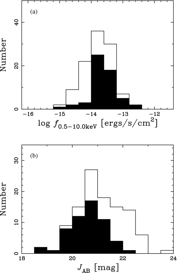
Figure 1. Selection and completeness of the COSMOS AGNs with FMOS spectra. Each panel shows the distribution of the observed sample (open histogram) and those that yield black hole mass estimates based on the Hα emission line (filled black histogram) for (a) X-ray 0.5–10.0 keV flux and (b) J-band magnitude.
Download figure:
Standard image High-resolution imagePrior to our observations, we had no empirical assessment of the performance of FMOS; thus, AGNs were targeted to faint infrared magnitudes, now understood not to be feasible using the low-resolution mode for the faintest objects (JAB ∼ 23). As shown in Figure 1(b), we have had a reasonable level of success (71%) with the detection of broad emission lines at brighter magnitudes (JAB < 21.5). Unfortunately, the success rate is significantly lower at fainter magnitudes, thus dropping to 50% for the entire sample with JAB < 23. It is worth highlighting that a survey depth of JAB < 21.5 is about 2 mag fainter than current near-infrared spectroscopic observations of SDSS quasars (Shen & Liu 2012) at similar redshifts. In Figure 2, we demonstrate this by plotting the bolometric luminosity (based on L3000 and a bolometric correction of 5.15; Shen et al. 2011) of our AGNs compared to those from SDSS surveys.

Figure 2. Bolometric luminosity as a function of redshift for AGNs in COSMOS (red filled circles), ECDF-S (red open circles), and SDSS (gray and black symbols). Errors represent a 1σ uncertainty of measurements, excluding systematic errors, e.g., uncertainty of bolometric correction.
Download figure:
Standard image High-resolution imageGreene & Ho (2005) describe in detail the benefits of using Hα for black hole mass measurements. In particular, the Hα emission line is stronger (∼3 ×), and thus more easily detected as compared to Hβ. This is clearly evident from our observations. We successfully detect a broad Hα line in ∼50% of the cases (as mentioned above), while the detection of Hβ is very low (17%). Even so, we do detect Hβ in a fair number of cases up to z ∼ 2.6 that will be presented in the full emission-line catalog (J. D. Silverman et al., in preparation). Any future FMOS campaign designed to detect the Hβ emission line (both broad and narrow) should increase the exposure time significantly and/or use the high-resolution mode that has roughly three times higher throughput in the H band as compared to the low-resolution mode (see Figure 19 of Kimura et al. 2010).
3. SPECTRAL-LINE FITTING
We measure the properties of broad emission lines present in optical and near-infrared spectra to derive single-epoch black hole mass estimates. For the emission lines of interest here (i.e., Mg ii and Hα), we specifically measure the FWHM, total luminosity of the emission line in the case of Hα, and monochromatic continuum luminosity at 3000 Å. Due to the moderate luminosities of the AGN sample, there can be a non-negligible host galaxy contribution that impacts the estimate of the AGN continuum at redder wavelengths; therefore, we chose to use the Hα line flux rather than the continuum luminosity. Fortunately, the multi-wavelength photometry of the COSMOS, including the Hubble Space Telescope imaging, enables us to determine the level of such contamination that will be fully assessed in a future study. Emission lines are fit using a procedure as outlined below that enables us to characterize the line shape for even those that have a considerable level of noise.
Our fitting procedure of the continuum and line emission utilizes MPFITFUN, a Levenberg–Marquardt least-squares minimization algorithm as available within the IDL environment. Even though this routine has well-known computational issues, this algorithm is widely used due to its ease of use and fast execution time. The routine returns best-fit parameters and their errors as well as a measure of the goodness of the overall fit. We further describe the individual components required to successfully extract a parameterization of the broad component used in determining the virial masses. It is worth noting that each line has its own advantages and disadvantages that need to be considered carefully, especially when fitting data of moderate signal-to-noise ratios (S/Ns); average S/N ∼6 in the Hα line and ∼20 in the M ii line. A final inspection of each fit by eye is performed to remove obvious cases where a broad component is not adequately determined almost exclusively due to spectra having low S/N; ∼3 for the Hα line in near-infrared spectra and ∼5 for Mg ii line in optical spectra.
3.1. Hα
We perform a fit to the Hα emission line (if detected within the FMOS spectral window) in order to measure line width and integrated emission-line luminosity. Based on the spectroscopic redshift as determined from optical spectroscopy, we select the spectrum at rest wavelengths centered on the emission line and spanning a range that enables an accurate determination of the continuum characterized by a power law, fλ∝λ−α.
We employ multiple Gaussian components to describe the line profile. It is common practice to make such an assumption on the intrinsic shape of individual components even though it has been demonstrated that broad emission lines in AGNs are not necessarily of such a shape (e.g., Collin et al. 2006). The Hα line is fit with two or three Gaussians (including a narrow component) and the [N ii] λ6548,6583 lines with a pair of Gaussians. The ratio of the [N ii] lines is fixed at the laboratory value of 2.96. The narrow width of the [N ii] lines is fixed to match the narrow component of Hα. The width of the narrow components is limited to 420–800 km s−1 (a range not corrected for intrinsic dispersion). The velocity profile of the broad components is characterized by the FWHM, which is measured using either one Gaussian or the sum of two Gaussians. We then correct the velocity width for the effect of instrumental dispersion to achieve an intrinsic profile width. The Hα luminosity discussed throughout this work is the sum of the broad components.
There are cases for which the fitting routine returns a solution with the width of the narrow component pegged at the upper bound of 800 km s−1. It is worth highlighting that this minimization routine stops the fitting procedure when a parameter hits a limit; thus, the returned values are not the true best-fit values. For these, we inspect all fits by eye and decide whether such an additional broad component is real. For many cases, we can use the [O iii] λ5007 line profile, within the FMOS spectral window, to determine whether such a fit to the narrow line complex is accurate. In addition, we can use the available optical spectra for such comparisons. When the level of significance of the narrow line is negligible, we rerun the fitting routine and fix the narrow line width to the spectral resolution of FMOS, ∼420 km s−1. In Figure 3, we show three examples of our fits to the Hα emission line that span a range of line properties.

Figure 3. Examples of our fitting routine for the Hα line detected in COSMOS AGN. In the upper portion of each panel, the observed spectrum is shown in black with the best fit in red. The continuum (gray dashed line) and individual emission-line components (gray Gaussian curves) are also indicated, respectively. In the lower panels, the residuals are shown with the same scale as that of the upper panel.
Download figure:
Standard image High-resolution image3.2. Mg ii
We fit the Mg ii emission line, as done in Schramm & Silverman (2012), observed in the optical spectra primarily from zCOSMOS (Lilly et al. 2009), Magellan/IMACS (Trump et al. 2007), and SDSS (York et al. 2000). The emission line is modeled by a combination of one or two broad Gaussian functions to best characterize the line shape. We first remove the continuum (before attempting to deal with the emission lines) by fitting the emission in a window surrounding the line. As with Hα, a power-law function is chosen to best characterize the featureless, non-stellar light attributed to an accretion disk. We further include a broad Fe emission component based on an empirical template (Vestergaard & Wilkes 2001) that is convolved by a Gaussian of variable width and straddles the base of the Mg ii emission line. A least-square minimization is implemented to determine the best-fit parameters. When possible, we optimize the residuals of the fits on a case-by-case basis by trying to minimize the number of components. Absorption features are either masked out or interpolated across. The fit returns two parameters required for black hole mass estimates: FWHM and monochromatic luminosity at 3000 Å. Examples of our fits to the Mg ii line are presented in Figure 4.

Figure 4. Examples of our fits for the Mg ii line for the same AGN as shown in Figure 3. The top panel shows the spectral range around Mg ii. The best-fit model is indicated as a red solid line. The different components are as indicated: Fe emission (blue), pseudo-continuum (purple), and Gaussian components (green and brown). The residual is shown in the lower panel. In the upper right corner of each panel, we show the black hole mass distribution computed from our Monte Carlo tests based on the uncertainties of the line width and continuum luminosity measurements.
Download figure:
Standard image High-resolution image4. RESULTS
We can determine how closely the parameters (i.e., luminosity and FWHM) required to estimate single-epoch black hole masses agree between the Hα and Mg ii emission lines. Any systematic offset or inherent scatter may only add additional uncertainty to the derived masses. We essentially want to establish whether or not the kinematics of the BLR is consistent with photoionized gas in virial motion around the SMBH. We provide all measurements and derived masses in Table 1.
Table 1. Catalog of Emission-line Properties and Black Hole Masses
| CIDa | Field | R.A. | Decl. | z | log L (erg s−1) | log FWHM (km s−1) | log MBH (M☉) | |||
|---|---|---|---|---|---|---|---|---|---|---|
| (J2000) | (J2000) | Hα | 3000 Å | Hα | Mg ii | Hα | Mg ii | |||
| 178 | COSMOS | 149.58521 | +2.05114 | 1.350 | 43.76 ± 0.03 | 45.35 ± 0.03 | 3.685 ± 0.013 | 3.811 ± 0.079 | 8.68 ± 0.03 | 8.78 ± 0.16 |
| 5275 | COSMOS | 149.59021 | +2.77450 | 1.400 | 44.10 ± 0.13 | 45.50 ± 0.02 | 3.835 ± 0.028 | 3.973 ± 0.072 | 9.18 ± 0.09 | 9.18 ± 0.14 |
| 322 | COSMOS | 149.62421 | +2.18067 | 1.190 | 43.16 ± 0.14 | 45.02 ± 0.02 | 3.440 ± 0.044 | 3.581 ± 0.081 | 7.84 ± 0.12 | 8.17 ± 0.16 |
| 192 | COSMOS | 149.66358 | +2.08522 | 1.220 | 43.24 ± 0.14 | 45.05 ± 0.02 | 3.339 ± 0.075 | 3.490 ± 0.035 | 7.68 ± 0.17 | 8.00 ± 0.07 |
| 157 | COSMOS | 149.67512 | +1.98275 | 1.330 | 42.98 ± 0.13 | 44.84 ± 0.03 | 3.701 ± 0.040 | 3.632 ± 0.017 | 8.28 ± 0.11 | 8.19 ± 0.04 |
| 2138 | COSMOS | 149.70358 | +2.57808 | 1.550 | 44.00 ± 0.06 | 45.27 ± 0.03 | 3.535 ± 0.050 | 3.635 ± 0.068 | 8.50 ± 0.11 | 8.39 ± 0.14 |
| 5163 | COSMOS | 149.71725 | +2.86564 | 1.410 | 44.01 ± 0.04 | 45.51 ± 0.04 | 3.621 ± 0.009 | 3.663 ± 0.009 | 8.69 ± 0.03 | 8.56 ± 0.02 |
| 329 | COSMOS | 149.73896 | +2.22067 | 1.020 | 43.86 ± 0.02 | 45.07 ± 0.03 | 3.887 ± 0.022 | 4.028 ± 0.007 | 9.15 ± 0.05 | 9.09 ± 0.02 |
| 5230 | COSMOS | 149.78467 | +2.71933 | 1.320 | 44.43 ± 0.01 | 45.85 ± 0.01 | 3.657 ± 0.006 | 3.713 ± 0.084 | 8.99 ± 0.01 | 8.82 ± 0.15 |
| 216 | COSMOS | 149.79179 | +1.87289 | 1.570 | 43.12 ± 0.11 | 44.35 ± 0.02 | 3.356 ± 0.148 | 3.529 ± 0.091 | 7.65 ± 0.31 | 7.75 ± 0.17 |
| 222 | COSMOS | 149.82196 | +1.83867 | 1.340 | 43.26 ± 0.02 | 44.92 ± 0.04 | 3.576 ± 0.042 | 3.744 ± 0.032 | 8.18 ± 0.09 | 8.45 ± 0.07 |
| 206 | COSMOS | 149.83704 | +2.00886 | 1.480 | 43.54 ± 0.06 | 45.01 ± 0.02 | 3.446 ± 0.025 | 3.478 ± 0.087 | 8.07 ± 0.06 | 7.96 ± 0.16 |
| 208 | COSMOS | 149.85196 | +1.99844 | 1.230 | 44.19 ± 0.03 | 45.70 ± 0.02 | 3.771 ± 0.009 | 3.982 ± 0.080 | 9.10 ± 0.03 | 9.29 ± 0.15 |
| 1194 | COSMOS | 149.88100 | +2.45083 | 1.310 | 43.11 ± 0.05 | 44.85 ± 0.03 | 3.316 ± 0.039 | 3.552 ± 0.091 | 7.56 ± 0.09 | 8.03 ± 0.17 |
| 1129 | COSMOS | 149.89483 | +2.17447 | 1.310 | 43.08 ± 0.03 | 44.43 ± 0.02 | 3.977 ± 0.052 | 3.947 ± 0.062 | 8.90 ± 0.11 | 8.62 ± 0.12 |
| 499 | COSMOS | 149.91975 | +2.32747 | 1.460 | 43.86 ± 0.06 | 45.34 ± 0.02 | 3.668 ± 0.024 | 3.867 ± 0.032 | 8.70 ± 0.06 | 8.89 ± 0.06 |
| 452 | COSMOS | 150.00446 | +2.23708 | 1.410 | 43.06 ± 0.16 | 44.64 ± 0.03 | 3.460 ± 0.113 | 3.516 ± 0.091 | 7.83 ± 0.25 | 7.86 ± 0.17 |
| 142 | COSMOS | 150.05379 | +2.58967 | 0.700 | 43.68 ± 0.04 | 45.07 ± 0.03 | 3.397 ± 0.011 | 3.373 ± 0.037 | 8.04 ± 0.03 | 7.78 ± 0.07 |
| 108 | COSMOS | 150.05871 | +2.47742 | 1.250 | 43.61 ± 0.04 | 45.12 ± 0.03 | 3.040 ± 0.175 | 3.678 ± 0.053 | 7.27 ± 0.36 | 8.41 ± 0.10 |
| 463 | COSMOS | 150.09588 | +2.14517 | 1.320 | 42.75 ± 0.09 | 44.48 ± 0.04 | 3.317 ± 0.197 | 3.656 ± 0.086 | 7.37 ± 0.41 | 8.06 ± 0.17 |
| 255 | COSMOS | 150.10162 | +1.84836 | 1.660 | 44.15 ± 0.10 | 45.58 ± 0.04 | 3.326 ± 0.097 | 3.414 ± 0.068 | 8.15 ± 0.21 | 8.10 ± 0.13 |
| 112 | COSMOS | 150.10267 | +2.53031 | 1.320 | 44.04 ± 0.04 | 45.68 ± 0.02 | 3.582 ± 0.014 | 3.568 ± 0.029 | 8.62 ± 0.04 | 8.45 ± 0.06 |
| 1028 | COSMOS | 150.16175 | +1.87794 | 1.450 | 42.87 ± 0.13 | 44.44 ± 0.03 | 3.226 ± 0.201 | 3.444 ± 0.050 | 7.24 ± 0.42 | 7.62 ± 0.09 |
| 1044 | COSMOS | 150.24517 | +1.90008 | 1.560 | 43.95 ± 0.06 | 45.41 ± 0.02 | 3.545 ± 0.041 | 3.820 ± 0.055 | 8.50 ± 0.09 | 8.83 ± 0.11 |
| 1174 | COSMOS | 150.27888 | +1.95947 | 1.550 | 43.42 ± 0.07 | 45.07 ± 0.03 | 3.401 ± 0.060 | 3.410 ± 0.023 | 7.91 ± 0.13 | 7.85 ± 0.05 |
| 119 | COSMOS | 150.29971 | +2.50692 | 1.500 | 43.37 ± 0.08 | 44.84 ± 0.02 | 3.483 ± 0.102 | 3.466 ± 0.089 | 8.05 ± 0.21 | 7.86 ± 0.17 |
| 54 | COSMOS | 150.31192 | +2.03575 | 0.970 | 43.25 ± 0.04 | 44.46 ± 0.03 | 4.104 ± 0.041 | 4.001 ± 0.015 | 9.26 ± 0.09 | 8.75 ± 0.03 |
| 305 | COSMOS | 150.37658 | +1.71789 | 1.570 | 44.03 ± 0.04 | 45.41 ± 0.03 | 3.584 ± 0.034 | 3.715 ± 0.077 | 8.62 ± 0.07 | 8.62 ± 0.15 |
| 66 | COSMOS | 150.37825 | +2.19642 | 1.510 | 43.15 ± 0.10 | 44.53 ± 0.03 | 3.720 ± 0.112 | 3.780 ± 0.081 | 8.42 ± 0.24 | 8.34 ± 0.16 |
| 389 | COSMOS | 150.38675 | +1.96669 | 1.530 | 43.46 ± 0.04 | 45.01 ± 0.02 | 3.704 ± 0.053 | 3.740 ± 0.048 | 8.55 ± 0.11 | 8.48 ± 0.09 |
| 536 | COSMOS | 150.44958 | +2.24644 | 0.880 | 43.09 ± 0.03 | 44.68 ± 0.04 | 3.521 ± 0.026 | 3.502 ± 0.038 | 7.98 ± 0.06 | 7.85 ± 0.08 |
| 642 | COSMOS | 150.49562 | +2.41256 | 1.370 | 43.24 ± 0.06 | 44.88 ± 0.02 | 3.679 ± 0.055 | 3.773 ± 0.006 | 8.38 ± 0.12 | 8.49 ± 0.02 |
| 597 | COSMOS | 150.52617 | +2.24497 | 1.271 | 43.27 ± 0.05 | 44.69 ± 0.02 | 3.186 ± 0.023 | 3.210 ± 0.029 | 7.38 ± 0.05 | 7.27 ± 0.06 |
| 604 | COSMOS | 150.58183 | +2.28769 | 1.340 | 43.25 ± 0.16 | 44.71 ± 0.03 | 3.285 ± 0.024 | 3.510 ± 0.078 | 7.57 ± 0.10 | 7.88 ± 0.14 |
| 607 | COSMOS | 150.60971 | +2.32311 | 1.295 | 43.59 ± 0.04 | 45.16 ± 0.03 | 3.505 ± 0.013 | 3.407 ± 0.087 | 8.21 ± 0.04 | 7.89 ± 0.16 |
| 305 | ECDF-S | 53.03612 | −27.79289 | 0.544 | 43.40 ± 0.03 | 44.98 ± 0.03 | 3.874 ± 0.030 | 3.763 ± 0.034 | 8.87 ± 0.06 | 8.52 ± 0.13 |
| 345 | ECDF-S | 53.06750 | −27.65844 | 1.324 | 43.49 ± 0.09 | 45.02 ± 0.02 | 3.462 ± 0.067 | 3.581 ± 0.069 | 8.07 ± 0.15 | 8.16 ± 0.13 |
| 358 | ECDF-S | 53.08462 | −28.03750 | 1.624 | 43.31 ± 0.17 | 45.23 ± 0.02 | 3.419 ± 0.137 | 3.532 ± 0.049 | 7.88 ± 0.30 | 8.17 ± 0.16 |
| 375 | ECDF-S | 53.11038 | −27.67658 | 1.030 | 43.79 ± 0.05 | 45.18 ± 0.02 | 3.377 ± 0.088 | 3.480 ± 0.033 | 8.06 ± 0.18 | 8.04 ± 0.13 |
| 379 | ECDF-S | 53.11250 | −27.68481 | 0.737 | 43.32 ± 0.03 | 45.05 ± 0.02 | 3.947 ± 0.025 | 4.013 ± 0.067 | 8.98 ± 0.05 | 9.05 ± 0.14 |
| 391 | ECDF-S | 53.12492 | −27.75833 | 1.218 | 43.17 ± 0.11 | 44.69 ± 0.01 | 4.023 ± 0.138 | 3.729 ± 0.077 | 9.05 ± 0.29 | 8.30 ± 0.11 |
| 417 | ECDF-S | 53.15879 | −27.66253 | 0.837 | 43.33 ± 0.02 | 44.67 ± 0.03 | 3.630 ± 0.015 | 3.718 ± 0.108 | 8.33 ± 0.03 | 8.28 ± 0.17 |
| 712 | ECDF-S | 53.37054 | −27.94483 | 0.840 | 42.67 ± 0.08 | 44.87 ± 0.02 | 3.782 ± 0.068 | 3.809 ± 0.018 | 8.28 ± 0.15 | 8.55 ± 0.14 |
Download table as: ASCIITypeset image
4.1. Luminosities
Our first concern is to determine whether the Hα emission-line luminosity scales appropriately with the UV continuum luminosity. For the following analysis, we do not correct for extinction due to dust and any contamination by the host galaxy; the impact of these, thought to be small, will be quantified in a later study. In Figure 5, the continuum luminosity, λLλ at 3000 Å, is plotted against the emission-line luminosity of Hα. Our data (as shown by the red points) spans two decades in luminosity and exhibits a clear correspondence between continuum and line emission. Based on our AGN sample, we determine the best-fit linear relation to be log (λL3000) = (0.82 ± 0.08) × log LHα + (9.31 ± 3.47). For the linear fitting, we adopt a FITEXY method (Press et al. 1992; Park et al. 2012). The level of dispersion of the data about this fit that will contribute to the dispersion in the final mass estimates is 0.20 dex.

Figure 5. Comparison between the monochromatic luminosity at 3000 Å and the Hα emission-line luminosity. AGNs in our sample are shown as red circles. The gray and black circles mark published observations of SDSS quasars (gray circles: 0.35 < z < 0.40; black circles: 1.5 < z < 2.2). A linear fit to both our data only (red line) and the joint sample (black line) is given. The distribution of log (λL3000/LHα) as a histogram is shown in the sub-panel. The colors of their histograms are the same as the symbols. Errors represent a 1σ level of uncertainty.
Download figure:
Standard image High-resolution imageWe can compare our data set to more luminous quasars from the SDSS. In particular, we identify 327 quasars from the SDSS sample in Shen et al. (2011) with 0.35 < z < 0.40 that cover a similar luminosity range as our high-redshift sample. These were selected from 1178 quasars at 0.35 < z < 0.40 based on high-quality data determined by adopting the following criteria: error in log (MBH/M☉) < 0.5, log (FWHMHα/km s−1) > 2.9, and . In addition, we include data from a recent study by Shen & Liu (2012) that provide the emission-line properties, including the Hα line of high-luminosity quasars from the SDSS with 1.5 < z < 2.2. These samples are added to our data shown in Figure 5. We clearly see that SDSS quasars fall along the λL3000–LHα relation as established above. Furthermore, the SDSS quasars have similar dispersion at both low-z and high-z samples to our sample, σ = 0.20 and σ = 0.15, respectively. We highlight that our AGN sample nicely extends such comparisons between continuum luminosity and line emission at higher redshifts and to lower luminosities. We are able to effectively establish a wider dynamic range that is not present in the high-z SDSS sample due to the limited luminosity range around log (λL3000) ∼ 46.2. By merging all three samples, we find the following relation based on a linear fit: log (λL3000) = (0.96 ± 0.01) × log LHα + (3.00 ± 0.53).

While there is very good agreement between the UV continuum and emission-line luminosity, there is a small difference that may impact, even slightly, our comparison of the masses. Based on the FMOS sample, the mean ratio 〈log (λL3000/LHα)〉 is 1.54 ± 0.03, which is slightly higher than that found for both the low-z and high-z SDSS quasar samples mentioned above; 〈log (λL3000/LHα)〉 = 1.40 ± 0.01 and 〈log (λL3000/LHα)〉 = 1.36 ± 0.02, respectively. This can be seen in the inset histogram in Figure 5. If this was due to the effect of dust extinction, then one would find the opposite trend with reduced UV continuum relative to the Hα line emission. There may be other explanations, such as an underlying spectral energy distribution that may be different for X-ray-selected samples (Elvis et al. 2012; Hao et al. 2012) and which has an impact on the response seen in photoionized gas, or the effect of the host galaxy on the aperture corrections that differ in each band. While this issue is important, we reserve a detailed investigation for subsequent work since it is beyond the scope of this paper to adequately demonstrate such effects. Here, we are primarily concerned with the magnitude of a luminosity offset and whether it contributes to an offset between the masses. With the black hole mass scaling with the square root of the luminosity (see below), the offset in luminosity, as determined above, amounts to a very small offset of 0.07 in log (MBH/M☉).
4.2. Velocity Widths
A second pillar for the use of Mg ii as a black hole mass indicator is that the emitting-line gas is located essentially within the same clouds that emit Balmer emission. While there are claims that this is the case by comparing the velocity profile of Mg ii with Hβ (e.g., McLure & Jarvis 2002; Shen et al. 2011), there are reported differences and trends that are not well understood (Wang et al. 2009; Shen & Liu 2012; Trakhtenbrot & Netzer 2012). For example, Mg ii tends to be narrower than Hβ, with a difference significantly larger at higher velocity widths (see Figure 2 of Wang et al. 2009).
Our aim here is to compare the FWHM of the Mg ii and Hα emission lines using a sample not yet explored, namely, the moderate-luminosity AGNs at high redshifts in survey fields such as COSMOS. In Figure 6, we plot the emission-line velocity width between Hα and Mg ii emission lines. Based on the FMOS sample only, a positive linear correlation is seen between the velocity width of the two emission lines with the mean ratio of (σ = 0.143). Our data is in very good agreement with those from the SDSS, i.e., (σ = 0.176) for the low-z sample from Shen et al. (2011), (σ = 0.076) for the high-z sample from Shen & Liu (2012), and recent FMOS results from Subaru XMM-Newton Deep Survey (see Nobuta et al. 2012). Based on a linear fit to the data shown in Figure 6, we measure a slope that is consistent with unity; (0.898 ± 0.132 for FMOS only and 1.001 ± 0.001 for FMOS+SDSS), and that cannot substantiate the claim by Wang et al. (2009) for a shallower value. These results support a scenario where the Mg ii and the Hα emitting regions are essentially cospatial with respect to the central ionizing source.


Figure 6. Comparison between the FWHM of Hα with that of Mg ii. The red, gray, and black circles are the same as those in Figure 5. A linear fit to both our data only (red line) and the joint sample (black line) is very similar to a one-to-one relation indicated by the dashed line. The distribution of is also shown in the sub-panel.

Download figure:
Standard image High-resolution imageThere are a few noticeable outliers well outside the dispersion of the sample. These objects then appear as outliers when comparing their masses based on different lines in the next section. Upon inspection, we find that these are the result of the FMOS spectra having low S/N. In some cases, there may be a fit to the Hα emission line, based on different parameter constraints, that is equally acceptable to the original fit as assessed by a chi-square goodness of fit and has a velocity width in closer agreement with Mg ii. However, we refrain from such selective fitting in order to present results that may be obtained from using similar fitting algorithms on larger data sets where such close inspection is not feasible.
4.3. Virial Single-epoch Masses
We now calculate black hole masses (MBH) based on our single-epoch spectra using both (1) L3000 and FWHM, and (2) LHα and FWHMHα. This calculation can be expressed as follows:


We explicitly use the recipes provided by Greene & Ho (2005) and McLure & Dunlop (2004) for the cases of the Hα and Mg ii lines, respectively:

We note that the calibration of the relation for Mg ii has been carried out by many studies (e.g., Vestergaard & Peterson 2006; McGill et al. 2008) and there are known differences between them.
In Figure 7, we show MBH for our sample derived from Hα and Mg ii. Our sample spans a range of 7.2 ≲ log (MBH/M☉) ≲ 9.5 that is consistent with that reported by previous studies of type 1 AGNs in COSMOS (Merloni et al. 2010; Trump et al. 2011) and that is complementary to the higher-L quasar sample at similar redshifts with log (MBH/M☉) ≳ 9 (Shen & Liu 2012). We find that the average (dispersion) in the black hole mass ratio of is 0.17 (σ = 0.32) for our FMOS sample. These results are similar to that determined from the SDSS sample; the average (dispersion) in the black hole mass ratio is −0.05 (σ = 0.39) at low z and −0.03 (σ = 0.20) at high z. While an offset of 0.17 dex is seen in the FMOS sample, we conclude that the recipes established using local relations give consistent results between Mg ii- and Hα-based estimates.


Figure 7. Comparison of the black hole mass estimated by Hα line with that by Mg ii line. The red, gray, and black circles are the same as those in Figure 5. The fit to both our data (red line) and the joint sample (black line) is nearly equivalent to a one-to-one relation (dashed line). The distribution of is also shown in the sub-panel.

Download figure:
Standard image High-resolution image
5. CONCLUSIONS
We have investigated the emission-line properties of AGNs in COSMOS and ECDF-S to establish whether Mg ii and Hα provide comparable estimates of their black hole mass. This study is the first attempt to do so for AGNs of moderate luminosity, and hence lower black hole mass (107 M☉ < MBH < 109 M☉), at high redshift that complements studies of more luminous quasars. Our results clearly show that the velocity profiles of Mg ii and Hα are very similar when characterized by FWHM and that the relation between continuum luminosity and line luminosity is tight. We then find that virial black hole masses based on Mg ii and Hα have very similar values and a level of dispersion (σ ∼ 0.3) comparable to luminous quasars from SDSS. It is important to keep in mind that these results pertain to specific calibrations (McLure & Dunlop 2004; Greene & Ho 2005) for estimating black hole mass. The use of other recipes, such as those provided by McGill et al. (2008), will show a discrepancy larger than seen here. In conclusion, the locally calibrated recipes for black hole masses using Mg ii and Hα are applicable for fainter AGN samples at high redshift. These results further support a lack of evolution in the physical properties of the BLR in terms of quantities such as αox (e.g., Steffen et al. 2006; Green et al. 2009), emission-line strengths (e.g., Fan 2006), and the inferred metallicities (Maiolino et al. 2001; Nagao et al. 2006; Matsuoka et al. 2011).
As a final word of caution, such estimates of black hole mass are likely to have inherent dispersion, as discussed above, and systematic uncertainties that are not yet well understood. For instance, recipes for estimating black hole mass depend on the assumption that the gas is purely in virial motion. This is unlikely to be true for all cases since both outflows and inflows are common in AGNs. Even so, there is evidence that the virial product of mass and luminosity (as a proxy for the radius to the BLR) is a useful probe of the central gravitational potential. In the very least, it is important to establish the level of dispersion in such relations since observed trends usually rely on offsets comparable to the dispersion such as the redshift evolution of the relation between black holes and their host galaxies (e.g., Peng et al. 2006; Merloni et al. 2010; Schramm & Silverman 2012).
We thank Kentaro Aoki and Naoyuki Tamura for their invaluable assistance during our Subaru/FMOS observations. K.M. acknowledges financial support from the Japan Society for the Promotion of Science (JSPS). T.N. is financially supported by JSPS (grant No. 23654068). Data analyses were carried out in part on common-use data analysis computer system at the Astronomy Data Center, ADC, of the National Astronomical Observatory of Japan (NAOJ).