


ABSTRACT
A proper understanding of the effects of turbulence on the diffusion and drift of cosmic rays (CRs) is of vital importance for a better understanding of CR modulation in the heliosphere. This study presents an ab initio model for CR modulation, incorporating for the first time the results yielded by a two-component turbulence transport model. This model is solved for solar minimum heliospheric conditions, utilizing boundary values chosen so that model results are in reasonable agreement with spacecraft observations of turbulence quantities in the solar ecliptic plane and along the out-of-ecliptic trajectory of the Ulysses spacecraft. These results are employed as inputs for modeled slab and two-dimensional (2D) turbulence energy spectra. The modeled 2D spectrum is chosen based on physical considerations, with a drop-off at the very lowest wavenumbers. There currently exist no models or observations for the wavenumber where this drop-off occurs, and it is considered to be the only free parameter in this study. The modeled spectra are used as inputs for parallel mean free path expressions based on those derived from quasi-linear theory and perpendicular mean free paths from extended nonlinear guiding center theory. Furthermore, the effects of turbulence on CR drifts are modeled in a self-consistent way, also employing a recently developed model for wavy current sheet drift. The resulting diffusion and drift coefficients are applied to the study of galactic CR protons and antiprotons using a 3D, steady-state CR modulation code, and sample solutions in fair to good agreement with multiple spacecraft observations are presented.
Export citation and abstract BibTeX RIS
1. INTRODUCTION
Diffusion and drift play key roles in the modulation of cosmic rays (CRs) in the heliosphere. Many scattering theories from which diffusion coefficients could be derived (see, e.g., Shalchi 2009) are available, but these theories require some form of turbulence power spectrum as a key input, which in turn depends on the nature of the turbulence in the heliosphere. Turbulence properties are relatively well understood at 1 AU (see, e.g., Bruno & Carbone 2005; Matthaeus & Velli 2011), but considerably less so elsewhere in the heliosphere. Herein lies the difficulty in applying the results of any scattering theory to the study of CR modulation: the need to self-consistently model various turbulence quantities so as to be in agreement with extant spacecraft data, and hence model the behavior of turbulence power spectra throughout the entire heliosphere. With the development of turbulence transport models (TTMs) of ever-increasing refinement (see, e.g., Zank et al. 1996, 2012; Breech et al. 2008; Oughton et al. 2011), this endeavor has become possible. Previous applications of such theories to the study of CR modulation, however, have been relatively few (e.g., Minnie et al. 2003, 2005; Burger & Visser 2010; Pei et al. 2010) and limited to single-component TTMs such as that of Breech et al. (2008).
This paper aims to outline the process involved in applying the results of the two-component TTM derived by Oughton et al. (2011), by means of chosen forms for turbulence power spectra, to the study of CR modulation in as self-consistent a way possible, employing diffusion coefficients derived from theory with these power spectra as inputs. Numerical particle simulations have shown that the effects of drift are reduced in the presence of turbulence (see, e.g., Minnie et al. 2007b). This paper also outlines how the results of the TTM employed can be used with the turbulence-reduced drift coefficient presented by Burger & Visser (2010), and considers its effect on CR modulation.
Section 2 will briefly discuss the forms for the slab and two-dimensional (2D) turbulence power spectra chosen for this study, as well as the TTM model used to provide inputs for these spectra, presenting a set of boundary values that lead to reasonable agreement with spacecraft data during solar minimum conditions. Section 3 will introduce and discuss the diffusion and drift coefficients employed. The effects of these coefficients on galactic proton modulation as computed with a 3D, steady-state CR modulation code for solar minimum conditions will then be discussed in Section 4. The paper closes with a summary and some concluding remarks in Section 5.
2. TURBULENCE TRANSPORT MODEL
As a point of departure, we specify a total turbulence modal spectrum such that G(k) = Gslab(k∥)δ(k⊥) + G2D(k⊥)δ(k∥), using the slab modal spectrum of Teufel & Schlickeiser (2003), based on the results of Bieber et al. (1994), such that
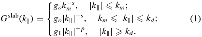
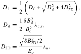
Here km = 1/λsl is the parallel wavenumber associated with the slab bendover scale λsl, and hence with the onset of the inertial range, kd = 1/λd is the wavenumber associated with the onset of the dissipation range,  , and
, and
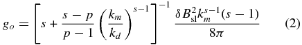
with  denoting the slab variance. The spectral index in the inertial range is denoted by s and is assumed to have a value of 5/3, and in the dissipation range it is denoted by p.
Assuming a flat energy range for the omnidirectional energy spectrum, one can define a 2D modal spectrum with an inertial range, an energy containing range, and an "outer range" displaying a steep decrease at the smallest wavenumbers, following Matthaeus et al. (2007), as
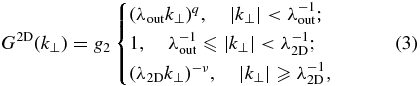
where  . Taking into account that
  ,
,
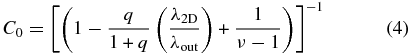
with the 2D bendover scale and the outer scale denoted by λ2D and λout, respectively, while the inertial range spectral index is denoted by ν, assumed here to be 5/3. The spectral index q of the outer range is set here as 3, again after Matthaeus et al. (2007). This 2D spectrum is different from that employed by, e.g., Pei et al. (2010) as it includes a well-defined energy range. Note that no dissipation range is defined, as the emphasis of this work will be on the effects of the large-scale/small-wavenumber behavior of the spectrum. The spectral form given in Equation (3) was chosen based on physical considerations discussed by Matthaeus et al. (2007), and due to the fact that the 2D ultrascale calculated from it is non-divergent, as opposed to that calculated from a spectrum that assumes finite values at zero wavenumber. The 2D ultrascale is given by
and is calculated as discussed by Matthaeus et al. (2007).
To employ the above spectra as inputs for mean free paths to be used in the heliospheric diffusion tensor, the various turbulence quantities that these spectra are functions of need to be modeled throughout the heliosphere. To this end, the two-component TTM of Oughton et al. (2011) is employed. This model was chosen for several reasons. First, using a single-component model like that of, e.g., Breech et al. (2008), which only describes the spatial variation of quasi-2D quantities, one would have to make relatively ad hoc assumptions as to the behavior of wavelike or slab quantities. The quasi-2D and wavelike turbulence quantities can also be treated as 2D and slab quantities in fair approximation (S. Oughton 2011, private communication), the set of fluctuations described by the slab/2D model being essentially a subset of those described by the quasi-2D/wavelike model (Oughton et al. 2006). This facilitates their use as inputs for extant CR scattering theories (see, e.g., Shalchi 2009). Second, the two-component approach allows for the assignation of energy due to turbulent driving processes to the appropriate component. The energy generated by the formation of pickup ions, previously assigned to the quasi-2D component in the models of, e.g., Zank et al. (1996), Smith et al. (2001), Smith et al. (2006), and Breech et al. (2008), can now be assigned more properly to the wavelike component (see, e.g., Hunana & Zank 2010; Oughton et al. 2011; Zank et al. 2012). Lastly, the relative ease with which the equations of the Oughton et al. (2011) model can be solved numerically greatly facilitates its application to the study of global CR modulation. Note that this model only yields the radial evolution of turbulence quantities at a particular colatitude, and that no latitudinal turbulence transport effects are considered. The equations constituting the Oughton et al. (2011) TTM are given by
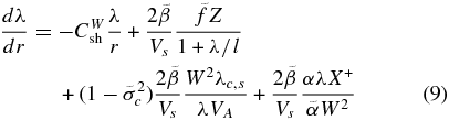
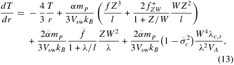
where Z2 and W2 denote the energies in quasi-2D and wavelike fluctuating components, respectively. Note that some of the variables used here are denoted differently from those in the equations presented by Oughton et al. (2011) so as to reflect their usage in this study. For more information as to this description of solar wind turbulence, see Oughton et al. (2004, 2006). In the above, λ and l represent correlation scales, perpendicular to an assumed uniform heliospheric magnetic field (HMF) component Bo, associated with the quasi-2D and wavelike fluctuating components, respectively, while λc, s represents the correlation scale parallel to Bo associated with the W2 component. As no observations currently exist to distinguish between λ and l (Oughton et al. 2011), the 2D correlation length is treated as a center-of-mass type average of l and λ, such that
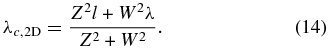
The normalized cross-helicities σc and  , again respectively associated with the Z2 and W2 components, are also solved for in this study, although these values are not in any way employed as inputs for the power spectra discussed above. Lastly, the symbol T denotes the solar wind proton temperature. For more insight into the physical significance of each term in the above equations and their derivation, the reader is referred to Oughton et al. (2011).
These equations are solved, utilizing a standard fourth-order Runge–Kutta scheme, for solar minimum heliospheric conditions. A hyperbolic tangent function is used to model the latitudinal solar wind speed profile, which assumes a value of 800 km s−1 over the solar poles and 400 km s−1 in the ecliptic plane, as reported by, e.g., McComas et al. (2000). This profile is shown in Figure 1. The solar wind speed Vsw is assumed to be independent of radial distance, so as to be consistent with the assumptions made in the derivation of the TTM. Similarly, the solar wind proton density ρ is assumed to scale as r−2. At Earth, the solar wind density ranges in value from ∼5 to 10 cc−1 (see, e.g., Smith et al. 2001), and is chosen to be 7 cc−1, and modeled to decrease with increasing solar wind speed, with a value of 2.7 cc−1 over the poles (see, e.g., McComas et al. 2000). The HMF is assumed to be an unmodified Parker (1958) field, with a magnitude of 5 nT at Earth (see, e.g., Jokipii 2001), while the Alfvén speed VA is calculated using the assumed model for the HMF and the solar wind proton density. Furthermore, a spherical heliosphere with no termination shock is assumed, with the inner boundary set at 0.3 AU and the outer boundary at 100 AU, as in, e.g., Breech et al. (2008) and Oughton et al. (2011).
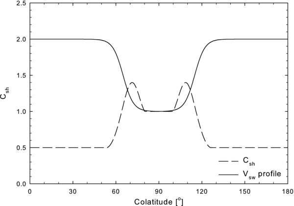
Figure 1. Solar wind speed and shear profiles used in this study as a function of colatitude.
Download figure:
Standard image High-resolution imageTurbulence-related quantities in the ecliptic plane are treated following the approach of Oughton et al. (2011) to a large degree. The de Kármán–Taylor constants α and β are assumed to be related by α = 2β, with α chosen to be equal to 0.125, as done by Pei et al. (2010). The wavelike analogs to these constants,  and
and  , are taken here to be equal to the de Kármán–Taylor constants in the equations governing the quasi-2D quantities (Oughton et al. 2011). The normalized energy difference σD is chosen to be a constant −1/3 following the approach of Breech et al. (2008). The terms
  and
and  model driving due to large-scale stream shear instabilities, and here, as in Oughton et al. (2011), it is assumed that
  . Furthermore, the colatitudinal dependence of the shear constants is very similar to that employed by Breech et al. (2008), and is shown in Figure 1: below a colatitude of ∼55° and above ∼125°, the shear constant is assumed to have a value of 0.5, while in the ecliptic plane it is assumed to be equal to one. At intermediate colatitudes, the shear profile used in this study increases to a value of 1.4 (as opposed to the value ∼1.6 assumed by the Breech et al. (2008) shear profile) due to the increased shear in this region. Note that here, as in Breech et al. (2008), no radial dependence is assumed for the shear constants. The geometrical mixing term M is taken to be M = cos 2ψ (Breech et al. 2008), and is allowed to vary throughout the heliosphere with the HMF winding angle ψ. This is different from the approach taken in previous studies where M was assumed to be equal to 1/2 throughout the heliosphere, a value corresponding to the magnitude of the winding angle at Earth. The term
  models the energy injected into the W fluctuations due to the formation of pickup ions, and is treated here exactly as discussed by Oughton et al. (2011), as is the resonant parallel length scale λres at which energy that is generated in the formation of the pickup ions would appear in the wavelike component's spectrum. The assumed ionization cavity scale Lcav is set at 5.6 AU.
A proper choice of boundary values is crucial to any attempt at finding agreement between model outputs and spacecraft data. Due to the relatively recent publication of the Oughton et al. (2011) transport model, there are not many sets of boundary conditions currently published. The values chosen here are somewhat different from those of Oughton et al. (2011), and are listed in Table 1. The main reason for this is that boundary values for the various length scales were set here so as to agree with the newest observational values at Earth for these quantities reported by Weygand et al. (2011), as opposed to the Weygand et al. (2009) observations used by Oughton et al. (2011). Due to the nature of the equations to be solved, this necessitated further changes in the boundary values chosen for other quantities. The boundary values for the quasi-2D fluctuation energy at 1 AU were chosen so that Z2 accounts for approximately 80% of the total energy, as observed by Bieber et al. (1994) following the approach of Oughton et al. (2011). The boundary values chosen for the respective normalized cross-helicities are the same as those chosen by Breech et al. (2008). The enhanced values of the fluctuation energies, however, motivated a lower choice for the initial value of the solar wind proton temperature than that used by Oughton et al. (2011) and required a different choice of de Kármán–Taylor constants. Note that boundary conditions were set so as to agree with solar minimum turbulence data wherever possible.
Table 1. Boundary Values Assumed at 0.3 AU for the Two-component Turbulence Transport Model
| Quantity | Units | Ecliptic Values | Polar Values |
|---|---|---|---|
| Z2 | km2 s−2 | 1250 | 1600 |
| W2 | km2 s−2 | 350 | 3000 |
| λ | AU | 0.004 | 0.015 |
| l | AU | 0.004 | 0.015 |
| λc, s | AU | 0.011 | 0.011 |
| σc | None | 0.6 | 0.8 |
 |
None | 0.6 | 0.8 |
| T | K | 2 × 10⁵ | 1.6 × 10⁶ |
Download table as: ASCIITypeset image
Figure 2 shows the various solutions of the Oughton et al. (2011) TTM in the solar ecliptic plane as a function of heliocentric radial distance. Panel (a) shows the magnetic variances calculated from the fluctuation energies W2 and Z2. Note that the variances corresponding to each component can be rather simply acquired by solving, e.g.,
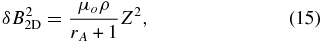
following Minnie (2006), where μo is the permeability constant and rA is the Alfvén ratio set to a value of 0.5 in this study (see, e.g., Roberts et al. 1987a, 1987b). The wavelike variance initially decreases steadily as a function of radial distance, but becomes flatter beyond ∼5 AU. This behavior is due to the action of  , which steadily becomes more significant at radial distances beyond the assumed ionization cavity scale Lcav. The pickup-ion term is not present in the quasi-2D fluctuation energy equation and hence the magnetic variance associated with it monotonically decreases with increasing radial distance. This result is consistent with the theoretical findings of Hunana & Zank (2010). It is an interesting consequence of this that the slab/2D anisotropy usually observed at Earth (e.g., Bieber et al. 1994) effectively reverses beyond ∼5 AU, a result first found by Oughton et al. (2011). The total magnetic variance is calculated as the sum of the quasi-2D and wavelike variances, and follows the trend of the Zank et al. (1996) Voyager data. Due to the action of the pickup-ion term on the wavelike component, it subsequently is dominated by the wavelike variance beyond ∼10 AU. The correlation scales are depicted in panel (b) of Figure 2 along with various observations. At 1 AU, both the parallel and perpendicular correlation length scales agree well with the observations for these quantities reported by Weygand et al. (2011). The Voyager values reported by Matthaeus et al. (1999) and Smith et al. (2001) are more properly to be compared with the perpendicular scales due to the geometry of the HMF beyond ∼2–10 AU (Zank et al. 1996; Oughton et al. 2011). These observations are not sufficient to allow one to distinguish as to whether they pertain to the perpendicular scale corresponding to the wavelike or the quasi-2D fluctuating components. Hence these points, as in Oughton et al. (2011), are compared here with a center-of-mass style-weighted average of the perpendicular length scales λc, 2D calculated according to Equation (14). This quantity appears to follow the radial trend of the data reasonably well, but appears to be too small by a factor of approximately two. It is worthwhile to note, however, that Matthaeus et al. (2005) report an overestimation by a factor of 2–4 of correlation scales observed using single-spacecraft data, compared with the observations acquired with multiple spacecraft, similar to the behavior of this quantity discussed by Oughton et al. (2011).
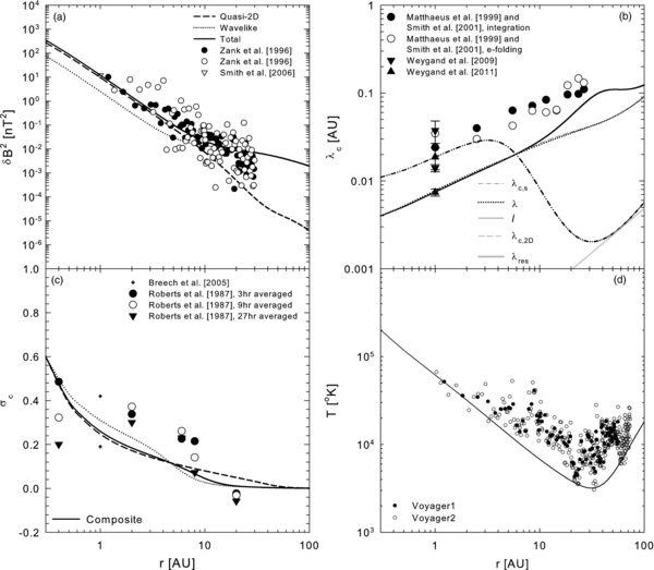
Figure 2. Various solutions of the two-component Oughton et al. (2011) turbulence transport model with assorted data, shown for an assumed Parker HMF, as a function of radial distance in the solar ecliptic plane. Panel (a) shows the variances associated with the wavelike and quasi-2D components, as well as the total variance, with data from Zank et al. (1996), and one point discussed in the text, from the results presented by Smith et al. (2006); panel (b) shows the various correlation length scales, with observations from Matthaeus et al. (1999), Smith et al. (2001), and Weygand et al. (2011); panel (c) shows the normalized cross-helicities corresponding to each component of the model, as well as the composite cross-helicity (solid line), with data from Roberts et al. (1987a, 1987b) and Breech et al. (2005); and panel (d) shows the modeled solar wind proton temperature, with data from Smith et al. (2001).
Download figure:
Standard image High-resolution imageThe normalized cross-helicities corresponding to the wavelike and quasi-2D fluctuations, as well as a composite cross-helicity defined as in Oughton et al. (2011), are shown in panel (c) of Figure 2 with data from Roberts et al. (1987a, 1987b) and Breech et al. (2005). All three quantities drop to values very close to zero within ∼50 AU, but the normalized cross-helicity associated with the quasi-2D fluctuations remains larger than zero for a larger radial distance than does that associated with the wavelike component. This is again due to the action of the pickup-ion term, in that the extra fluctuation energy added to the wavelike component acts so as to decrease the normalized cross-helicity associated with it. For the purposes of comparison with data, the composite cross-helicity remains within the range of almost all the data points, except the last triad at 20 AU. Panel (d) of the same figure shows the calculated solar wind proton temperature. The radial profile displayed agrees qualitatively with observations, in that for the inner heliosphere the expected adiabatic profile is reproduced, with an increase at higher radial distances due to the injection of energy into the wavelike component by the formation of pickup ions.
Oughton et al. (2011) only provide a set of boundary conditions applicable to the solar ecliptic region, whereas this study requires a set for all colatitudes considered. High-latitude comparisons of model outputs are made here with observations of the fluctuation energies, correlation scales, normalized cross-helicities, and solar wind proton temperatures taken by the Ulysses spacecraft and reported by Bavassano et al. (2000a, 2000b). The motivation behind the choices of inner boundary values made here has been to find agreement with these in situ data sets along the trajectory of the Ulysses spacecraft. This approach to finding boundary values at high latitudes for TTMs has not been taken before. Bavassano et al. (2000b) note that the turbulence in the high-latitude fast solar wind does not behave too differently from that present in low-latitude fast solar wind streams, and some of the choices made here take into account observations at Earth for such solar wind conditions. Inner boundary values for the wavelike and quasi-2D fluctuation energies were taken to assure a wavelike-dominated anisotropy, motivated by the findings of Weygand et al. (2011), although it is unclear as to what the exact proportions of the anisotropy are. Likewise, boundary values for the correlation scales were chosen so that model outputs would agree with correlation scales observed along the Ulysses trajectory. The boundary values for the correlation scales were also chosen so that the ratio of the wavelike correlation scale to the composite transverse scale yielded by the TTM would agree with the findings of Weygand et al. (2011). The values found by Weygand et al. (2011) for fast solar wind conditions at Earth are considerably lower than the observations of Bavassano et al. (2000a, 2000b). These latter observations were in situ, however, and so emphasis was placed on finding broad agreement with them, and not with the Weygand et al. (2011) findings. The boundary values assumed here at 0.3 AU are listed in Table 1. Note that latitudinal changes in boundary values, as with the solar wind speed profile, are effected here using hyperbolic tangent transition functions.
The trajectory followed by Ulysses was designed to consist of significant excursions in latitude during the so-called fast latitude scans. This can be seen as a function of time in the bottom panels of Figure 3. The same figure shows fluctuation energies, correlation scales, normalized cross-helicities, and the solar wind proton temperature yielded along the trajectory of Ulysses by the TTM, along with observations reported by Bavassano et al. (2000a, 2000b). Note that these data do not include observations taken in the ecliptic region, leading to a gap spanning about 45° in latitude centered on the ecliptic. Panel (a) of Figure 3 shows the fluctuation energies corresponding to both the quasi-2D and wavelike components with their sum. The observations taken by Bavassano et al. (2000a, 2000b) are assumed here to pertain to the energy due to all turbulent fluctuations. Both W2 and Z2 increase to peak values in approximately 1995. This increase is due to a combination of the latitudinal excursion of the spacecraft and the decrease in radial distance to be seen in the bottom panels of Figure 3. Shortly thereafter, a sharp "bump" is seen in Z2 at ∼1995.1 due to greater stream-shear effects at these latitudes. After ∼1995.1, both fluctuation energies exhibit steep drop-offs due to Ulysses approaching the ecliptic plane, for which the assumed boundary values for fluctuation energies are much lower. After passing the ecliptic, both quantities increase again, more or less mirroring the pre-ecliptic behavior, as Ulysses now approaches the "North" pole. That this mirroring is not exact is not due to any North–South asymmetries inherent to the model, but rather due to the somewhat asymmetric spacecraft trajectory. The sum of the fluctuation energies behaves similarly to its parts, and initially agrees well with the Bavassano et al. (2000a, 2000b) observations. As the spacecraft approaches the ecliptic, however, the model undershoots the data. This is due to the fact that boundary values in the ecliptic were chosen so as to acquire solutions in agreement with ecliptic data, taken using various spacecraft, techniques, and averaging times, which may not be completely comparable to the hourly averaged Bavassano et al. (2000a, 2000b) data. The model, however, agrees reasonably well with most of the observations, along a broad range of the varied spatial positions along the trajectory of Ulysses.

Figure 3. Fluctuation energies, correlation length scales, normalized cross-helicities, and solar wind proton temperature yielded by the two-component Oughton et al. (2011) turbulence transport model along the trajectory of the Ulysses spacecraft during its first fast latitude scan. Data shown are from Bavassano et al. (2000a, 2000b). Note the gap in the data in the region centered on the ecliptic plane and spanning ∼45° in latitude. The bottom two panels illustrate the radial and colatitudinal position of Ulysses.
Download figure:
Standard image High-resolution imageThe correlation scale observations of Bavassano et al. (2000a, 2000b), shown alongside the parallel and composite perpendicular correlation length scales (calculated with Equation (14)) yielded by the TTM in Figure 3, show a rather broad spread. This, coupled with the fact that it is difficult to say whether one should compare them with a perpendicular or a parallel correlation scale, makes it very hard to evaluate model results. Hence, the boundary values were set here so as to yield model results that for both length scales fall on the lowest values of the data, this being motivated by the reported overestimation of correlation scales acquired from single-spacecraft measurements (Matthaeus et al. 2005). Neither of these length scales is incompatible with the Bavassano et al. (2000a, 2000b) data. The ratio of the parallel to perpendicular correlation scales remains approximately 0.70 along most of Ulysses's trajectory considered here. This is due to the fact that at high latitudes, within the radial distances traversed by this spacecraft, both length scales yielded by the model have very similar radial dependences. The relatively gradual increase of these quantities with radial distance at high latitudes leads to the relatively flat pre-1995 model results. Beyond this, a sharp "bump" in the parallel correlation scale corresponding to regions of greater shear can be seen. At high latitudes, the composite perpendicular scale is consistently larger than the parallel correlation scale, but this scenario is reversed as model results closer to the ecliptic are considered, consistent with the results shown in panel (b) of Figure 2. The model results in the northern hemisphere approximately mirror those discussed above.
At higher latitudes and radial distances along Ulysses's trajectory, the normalized cross-helicity observations reported by Bavassano et al. (2000a, 2000b) show a fairly large spread. The TTM results, including the composite value shown in Figure 3, are well within the range of this data set, at least before 1994.6 and after 1995.5. Agreement, however, again worsens as the spacecraft approaches the ecliptic plane. The modeled normalized cross-helicity associated with both components exhibits a decrease in magnitude at times, such as ∼1995.1 and ∼1995.2, associated with regions of increased shear along the spacecraft trajectory, although the values yielded by the two-component model are far below the data at these latitudes. This is partly due to the fact that boundary values for the ecliptic plane were chosen so as to agree with the observational values reported by Roberts et al. (1987a, 1987b) and Breech et al. (2005). These ecliptic values were calculated for fluctuation spectra observed over periods of 3, 9, and 27 hr (the Roberts et al. 1987a, 1987b observations) and periods of 12 and 24 hr (the Breech et al. 2005 points), the value at each radial distance considered being quite sensitive to this period of observation. The Bavassano et al. (2000a, 2000b) normalized cross-helicities were calculated from hourly averaged data, and this difference may contribute to the lack of agreement between model outputs and data near the ecliptic. It may also be due to an inappropriate choice of one of the turbulence parameters here, such as Csh, significant in the streamer belt. The solar wind proton temperature yielded by the TTM, shown in Figure 3, agrees very well with the temperatures observed by Ulysses at higher latitudes and radial distances.
Figure 4 illustrates turbulence levels yielded by the Oughton et al. (2011) TTM, expressed as the ratio of the square root of the magnetic variance to the Parker HMF magnitude Bo at various colatitudes as functions of radial distance. Values considered by Minnie et al. (2007a) for the total turbulence level are shown for comparison in all three panels. At lower colatitudes, the total turbulence level, shown in panel (a), is dominated at all radial distances by the contribution from the slab component (shown in panel (c)). This is due, in the inner heliosphere, to the choice of boundary values at these colatitudes motivated above, and in the outer heliosphere due to the action of the pickup-ion term  . The 2D turbulence level, shown in panel (b) of Figure 4, steadily decreases in the outer heliosphere for all colatitudes shown, for the same reasons as outlined in the discussion of Figure 2.
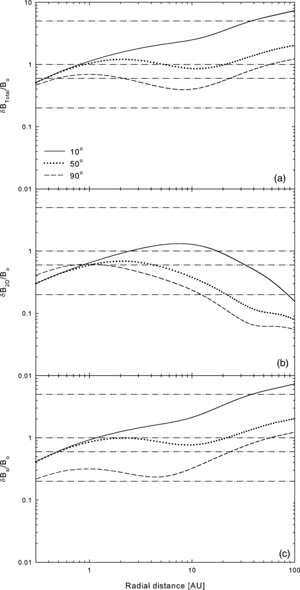
Figure 4. Turbulence levels yielded by the Oughton et al. (2011) TTM as a function of radial distance at various colatitudes. Panel (a) shows the total turbulence level, while panels (b) and (c) show respectively the 2D and slab levels. The dot-dashed lines indicate the total turbulence levels considered by Minnie et al. (2007a) in their numerical simulations of diffusion coefficients.
Download figure:
Standard image High-resolution imageThe turbulence quantities yielded by this transport model are used to calculate inputs to the turbulence power spectra. These spectra will be used in ab initio expressions for CR mean free paths, whose spatial dependences will now depend on the behavior of the solutions to the two-component TTM.
3. DIFFUSION AND DRIFT
The choice of scattering theory to be used is crucial to any study of CR modulation, affecting as it does the global behavior of the diffusion coefficients. This task, however, is rendered extremely difficult by the fact that one must somehow discriminate among several theories based on observations and test particle simulations applicable almost exclusively to conditions prevalent at Earth. Simulations such as those performed by, e.g., Minnie et al. (2007a) show that different scattering theories are more or less accurate in their description of simulated diffusion coefficients depending on the level of turbulence present. Figure 4 quite clearly shows that a large range of modeled turbulence levels can exist within the heliosphere. The turbulence levels considered by Minnie et al. (2007a) are shown in this figure as dot-dashed lines. As the accuracy of different theories depends on the level of turbulence, the implication is that there does not appear to be a "one size fits all" scattering theory. This is a further difficulty to be considered in the choice of a scattering theory to be used in CR modulation studies.
In this study, the quasi-linear theory (QLT) of Jokipii (1966) is used, following Bieber et al. (1994) in the assumption of composite turbulence, as the basis for modeling the parallel diffusion coefficient, employing expressions for the parallel mean free path based on the results of Teufel & Schlickeiser (2003), which are reported by Burger et al. (2008). This decision is motivated by the fair agreement with observations that parallel mean free paths derived from QLT show, as well as the reasonable agreement obtained for simulations with relatively low levels of turbulence (Minnie et al. 2007a). The higher levels of modeled slab turbulence in the outer heliosphere shown in Figure 4 would appear to render QLT a less optimal choice in this regard. However, CR modulation in this region would, due to the geometry of the HMF, be expected to be dominated by perpendicular diffusion and drift effects.
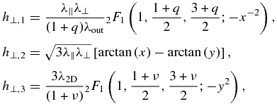
The Burger et al. (2008) proton parallel mean free path employed here is constructed from piecewise continuous expressions derived by Teufel & Schlickeiser (2003) using Equation (1), but neglecting the effects of the dissipation range, and is given by
where R = RLkm, with RL the (maximal) proton gyroradius. The turbulence-related quantities required by this expression are calculated from the solutions to the TTM discussed in the previous section.
For the perpendicular mean free path, the extended nonlinear guiding center (ENLGC) theory of Shalchi (2006), based on the nonlinear guiding center (NLGC) theory of Matthaeus et al. (2003), is employed. Not only do the predictions of this theory agree well with numerical simulations over a broad range of rigidities and turbulence levels, but it also successfully reproduces the relatively flat rigidity dependences observed for the perpendicular mean free path at 1 AU (see, e.g., Palmer 1982; Burger et al. 2000). Furthermore, the good agreement of ENLGC results with those of numerical simulations performed for slab-dominated composite turbulence as opposed to the results of the standard NLGC formulation reported by Shalchi (2006), given the slab-dominated scenario in the outer heliosphere yielded by the Oughton et al. (2011) model used in the present study, motivates the choice of this theory to describe perpendicular diffusion in the present study. The 2D power spectrum given in Equation (3) is used to derive a nonlinear perpendicular mean free path, following the approach of Shalchi et al. (2004) to some degree and assuming axisymmetric turbulence, given by
where
with
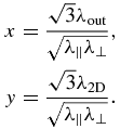
The parameter a2 is a constant, reported by Matthaeus et al. (2003) to have a value of 1/3. Note that the range of values proposed by Shalchi & Dosch (2008) would lead to larger perpendicular mean free paths. Equation (17) is evaluated numerically, using turbulence quantities calculated from the outputs of the TTM. The ENLGC perpendicular mean free path contains one important and essentially free parameter for which no direct observations exist, the 2D outer scale λout. This being the case, a very simple spatial dependence for this quantity is chosen here, such that λout = 12.5λc, 2D, and therefore λout > λ2D throughout the model heliosphere. This ensures a well-defined energy range on the assumed 2D power spectrum, an assumption implicit to the use of the Oughton et al. (2011) TTM.
Numerical simulations show that drift effects are reduced in the presence of turbulence (see, e.g., Minnie et al. 2007b). Here, a parameterized drift coefficient proposed by Burger & Visser (2010) that is both reduced in the presence of turbulence and approaches the weak scattering coefficient in the absence of turbulence is utilized. This particular coefficient was chosen due to its ability to reproduce the results of the simulations of both the drift coefficients and velocity reported by Minnie et al. (2007b). The drift coefficient in the presence of turbulence is given by (Bieber & Matthaeus 1997)
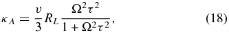
with τ being the decorrelation rate and Ω the particle gyrofrequency. Burger & Visser (2010) propose a parameterized form for the product Ωτ, given by
where g = 0.3log (RL/λc, s) + 1.0 and D⊥ is the field line random walk diffusion coefficient (see, e.g., Matthaeus et al. 1995):
Equations (16)–(18) describe an ab initio diffusion tensor when used in conjunction with the TTM model. A brief discussion of the rigidity and spatial dependences of the mean free paths and drift scale follows. Similar characterizations of these length scales have previously been published by, e.g., Zank et al. (1998) and Pei et al. (2010) using the single-component TTMs proposed by Zank et al. (1996) and Breech et al. (2008), respectively.
Sample mean free paths and drift scales corresponding to λout = 12.5λc, 2D are shown in Figure 5 as a function of rigidity, heliocentric radial distance, and colatitude. Panel (a) of this figure shows these length scales as a function of rigidity at Earth. The proton parallel mean free paths display a clear P1/3 rigidity dependence as expected, in qualitative agreement with the observations of, e.g., Dröge (2000), but remain above the Palmer (1982) consensus range. A possible factor to affect the mean free paths not fully considered by Palmer (1982) is the effect that the solar activity cycle would have on them. This would be somewhat masked in the observations of which the consensus is composed, as most solar particle events considered by Palmer (1982) and the studies referenced therein occurred during periods of ascending to high solar activity. Chen & Bieber (1993) find that at neutron-monitor energies larger mean free paths are associated with solar minima, and smaller mean free paths with solar maxima, and report a mean free path dependence on solar magnetic polarity. This would then imply that the Palmer consensus values may be a lower estimate for the parallel mean free path.
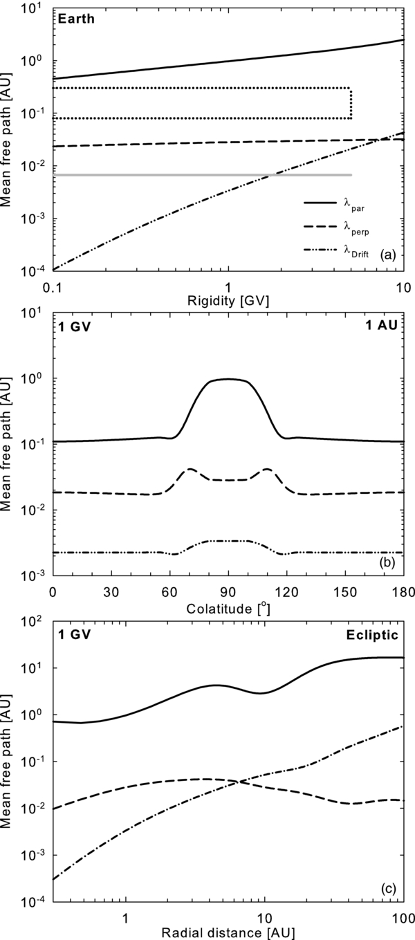
Figure 5. Parallel and perpendicular mean free paths, along with the drift scale, shown as functions of rigidity (top panel), colatitude at 1 AU (middle panel), and radial distance in the ecliptic plane (bottom panel). The Palmer (1982) consensus ranges for the parallel and perpendicular mean free paths are indicated in the top panel by the dotted box and gray line, respectively.
Download figure:
Standard image High-resolution imageThe perpendicular mean free paths remain relatively flat as a function of rigidity, similar to the results of Shalchi et al. (2004) and Pei et al. (2010), and in qualitative agreement with the findings of Burger et al. (2000), but remain well above the Palmer (1982) consensus range, due to the fact that the boundary values for the Oughton et al. (2011) model were chosen so that it yields larger turbulence quantities corresponding to solar minimum conditions. The 1 AU ecliptic perpendicular mean free paths shown here are similar to those presented by Pei et al. (2010), differing in magnitude due to the different TTMs employed by those authors. At the highest rigidities shown, the drift scale λA scales as RL, as expected of the weak scattering limit, deviating from this behavior only below ∼1 GV, where the drift-reduction effects of the modeled turbulence come into play.
Panel (b) of Figure 5 shows the 1 GV mean free paths and drift scale as a function of colatitude at 1 AU. The parallel mean free path is larger in the ecliptic region, where modeled slab variances are smaller, than over the poles, where the slab variances calculated from the results of the TTM are larger. This is in qualitative agreement with the findings of Erdös & Balogh (2005). This is also the case for the perpendicular mean free path and the drift scale. The perpendicular mean free paths follow the latitudinal profile of the 2D variance yielded by the Oughton et al. (2011) model, with larger values in the ecliptic than over the poles, and two "bumps" corresponding to the enhanced turbulence present in regions of greater modeled stream-shear effects. The drift scales are noticeably reduced at latitudes corresponding to regions of enhanced stream-shear effects, where turbulence levels are larger. It is also interesting to note that the drift scale colatitudinal profile is markedly different, due to the effects of turbulence, from that expected of RL, in that the latter quantity would be larger over the poles than in the ecliptic plane.
The ecliptic radial profiles of the 1 GV mean free paths and drift scale are shown in panel (c) of Figure 5. The parallel mean free path roughly resembles those reported by Pei et al. (2010) for the pickup-ion-driven single-component Breech et al. (2008) TTM. The parallel mean free path shown in Figure 5 increases steadily with increasing radial distance until ∼5–6 AU, reflecting the steady decrease of the slab variance and increase of the slab correlation scale shown in Figure 2. For a few astronomical units beyond this distance, corresponding roughly to the ionization cavity length scale of 5.6 AU assumed here, the parallel mean free path decreases somewhat due to the increased variance and decreased correlation scales caused by the ionization of interstellar neutral hydrogen. This decrease in the parallel mean free path, not seen in the results of Pei et al. (2010), is quite brief, and the parallel mean free path again increases with radial distance, as the slab variance remains at a relatively large value that decreases slowly with increasing radial distance, while the correlation scale here becomes proportional to the radially increasing resonant length scale λres at which energy due to the formation of pickup ions enters the slab fluctuation spectrum. At the largest radial distances, the parallel mean free path flattens out due to the combined effects of the increasing slab correlation scale and the decreasing slab variance. The perpendicular mean free path shows a steady increase with radial distance out to ∼4 AU, reflecting the increase in both the 2D correlation scale and parallel mean free path within this distance. Beyond this, however, the perpendicular mean free path decreases with radial distance, reflecting the radial behavior of the 2D variance calculated from the TTM. This decrease, however, is not as steep as might be expected, and reflects the radial behavior of the larger parallel mean free paths in the outer heliosphere discussed above. The perpendicular mean free path shown here is qualitatively similar to that presented by Pei et al. (2010) at smaller radial distances. In the outer heliosphere, however, the Pei et al. (2010) perpendicular mean free paths continue increasing with radial distance, while those presented here tend to decrease. This difference is due to the influence of the Breech et al. (2008) TTM employed by Pei et al. (2010), where the turbulence generated by pickup-ion formation enters the 2D component, leading to 2D variances that do not decrease as steeply with radial distance, as opposed to those yielded by the Oughton et al. (2011) model employed here, which assigns the energy due to pickup-ion formation to the slab component only. The drift scale increases monotonically, following the behavior of the 2D correlation scale shown in Figure 2.
4. COSMIC-RAY MODULATION
To investigate the effects of the diffusion tensor described in the previous sections on the modulation of galactic CR protons and antiprotons, a 3D, steady-state CR modulation code, used by Burger et al. (2008), is applied to solve the Parker (1965) CR transport equation for solar minimum conditions. Perpendicular diffusion is assumed to be axisymmetric, and the same Parker model as in the TTM is used to describe the HMF. Furthermore, a spherical heliosphere with a radius of 100 AU, which does not include a termination shock or heliosheath, is assumed. This is a limitation, in that observations and numerical simulations have shown that some modulation can occur within the heliosheath (see, e.g., Caballero-Lopez et al. 2010). Effects due to the heliosheath are, however, excluded for two reasons. First, the Oughton et al. (2011) TTM was derived assuming an Alfvén speed considerably smaller than the solar wind speed. This is not the case in the heliosheath. Second, not much is observationally known for certain as to the large-scale structures such as the HMF, solar wind, and current sheet profiles, beyond that which has been gleaned from Voyager data in the small region traversed by these spacecraft, with even less information available as to the turbulence conditions in this region. Various results of MHD simulations for the large-scale plasma quantities have been published (see, e.g., Florinski et al. 2011), but little observational data exist so as to allow for an accurate assessment of the results yielded by these simulations for a large part of the region they describe.
The effects of current sheet drift are treated following Burger (2012). The tilt angle of the heliospheric current sheet was taken to be 5°, the magnetic field magnitude at Earth was chosen to be 5 nT, and the solar wind profile was taken to be exactly the same as discussed in Section 2. Lastly, the proton local interstellar spectrum (LIS) is that used by Burger et al. (2008), which is similar to that of Bieber et al. (1999) at high energies, but assumes larger values at low energies. The antiproton LIS is that used by Langner & Potgieter (2004). The above-mentioned CR species are studied using the QLT and ENLGC diffusion coefficients as functions of turbulence quantities modeled using the two-component TTM. The same turbulence conditions and diffusion coefficients are assumed for each species considered.
Panel (a) of Figure 6 shows computed galactic proton differential intensity spectra as a function of kinetic energy at Earth, alongside various observations reported by McDonald et al. (1992; IMP8) and Shikaze et al. (2007; BESS97). We assumed that λout = 12.5λc, 2D, and this choice of 2D outer scale leads to results in fair agreement with the spacecraft observations for both magnetic polarity epochs (A > 0 and A < 0). Latitude gradients, shown at 2 AU so as to be comparable with Ulysses data reported by Heber et al. (1996) and de Simone et al. (2011), are illustrated as a function of rigidity in panel (b) of the same figure. Computed latitude gradients are calculated as in Burger et al. (2008). The ab initio approach yields latitude gradients reasonably within the range of observations during A > 0, even though a Parker HMF model is used and axisymmetric perpendicular diffusion is assumed. Computed A < 0 latitude gradients are negative but appear to be somewhat too large in absolute magnitude, overshooting the de Simone et al. (2011) data point. Computed antiproton differential intensities are shown as a function of kinetic energy, together with spacecraft observations reported by Orito et al. (2000), Maeno et al. (2001), and Adriani et al. (2010), in panel (c) of Figure 6. Intensities computed with the 3D modulation code during A < 0 are larger than those for A > 0, as expected for these negatively charged CRs. The amount of modulation and the separation between the modeled spectra at 1 AU are very small. This result is quite similar to that reported by Langner & Potgieter (2004). Furthermore, although the error bars on the observations are quite significant, it is encouraging to note that the results yielded by the ab initio 3D modulation code agree rather well with spacecraft data. The same can be said of the ratios of the computed antiproton to proton intensities at Earth, shown as a function of kinetic energy in panel (d) of Figure 6, which are in good agreement with the PAMELA observations reported by Adriani et al. (2009).

Figure 6. Computed galactic proton intensities (panel (a)) and latitude gradients (panel (b)). Spacecraft data shown are reported by McDonald et al. (1992; IMP8), Shikaze et al. (2007; BESS97), Heber et al. (1996; Ulysses), and de Simone et al. (2011; Ulysses/PAMELA). Panels (c) and (d) show respectively the computed antiproton intensities and antiproton/proton ratios, along with observations reported by Orito et al. (2000; BESS95 and BESS97), Maeno et al. (2001; BESS98), Adriani et al. (2010; PAMELA), and Adriani et al. (2009; PAMELA, antiproton/proton ratios).
Download figure:
Standard image High-resolution image
5. SUMMARY AND CONCLUSIONS
This study presents the first attempt at the self-consistent application of the results yielded by a two-component TTM to the ab initio study of CR modulation. This was done by solving the Oughton et al. (2011) TTM for typical solar minimum heliospheric conditions such that the turbulence quantities are in reasonable agreement with spacecraft observations taken in the solar ecliptic plane in general, and with observations taken along the trajectory of Ulysses. These turbulence quantities were then used as inputs for chosen forms for the slab and 2D turbulence power spectra, which in turn were used as inputs for parallel mean free path expressions based on the QLT results of Teufel & Schlickeiser (2003) and perpendicular mean free path expressions derived from the ENLGC theory of Shalchi (2006). To self-consistently incorporate the effects of the modeled turbulence on CR drifts, an expression for the 2D ultrascale was derived from the expression for the chosen 2D turbulence power spectrum. This spectrum was constructed, following Matthaeus et al. (2007), in such a way as to drop off at the lowest wavenumbers. This behavior, commencing at a wavenumber corresponding to what is termed as the 2D outer scale in this study, is physically motivated by Matthaeus et al. (2007) and ensures a non-diverging expression for the 2D ultrascale. As the 2D outer scale is a key component of the 2D turbulence power spectrum, the perpendicular mean free paths derived using such a spectrum will also be sensitive to this quantity's behavior. The 2D ultrascale is then used in expressions for the reduced drift coefficient proposed by Burger & Visser (2010), using again the results of the TTM to describe the relevant turbulence quantities. The drift and diffusion coefficients were then used in a 3D, steady-state numerical CR modulation code, assuming a relatively simple form for the 2D outer scale.
Galactic proton intensities computed following this approach were found to be in fair to good agreement with multiple sets of spacecraft observations taken at various locations in the heliosphere. An interesting result of the ab initio approach is the reduction in magnitude of computed proton latitude gradients, even when a pure Parker HMF model and axisymmetric perpendicular diffusion were assumed. This led to results that were in reasonable agreement with observations reported for this quantity for A > 0 by Heber et al. (1996). Computed latitude gradients for A < 0 appear to be too large in absolute value. This issue may be resolved in future by either an alternative spatial dependence for the 2D outer scale or the use of a turbulence-reduced drift coefficient other than the constructed form proposed by Burger & Visser (2010). Antiproton intensities were calculated employing exactly the same parameters that were used in the ab initio modulation model when protons were considered, and reasonable agreement with spacecraft observations was obtained. The good agreement of computed antiproton-to-proton ratios with spacecraft observations seems to imply that the ab initio approach employed here handles both species equally well.
To conclude, an ab initio treatment of diffusion and drift, incorporating in as self-consistent a way as possible the effects of turbulence as described by a two-component TTM, which is set in such a way as to yield results in reasonable to good agreement with spacecraft observations of turbulence quantities, can yield computed CR intensities in reasonably good agreement with multiple sets of spacecraft observations, and for different CR species.
Subsequent studies using this model will focus on the effect various forms of the 2D outer scale would have on CR modulation, and an application of the model to the study of the modulation of galactic electrons and positrons.
N. E. E. thanks Sean Oughton and John Bieber for helpful discussions. The financial assistance of the National Research Foundation (NRF) toward this research is hereby acknowledged. Opinions expressed and conclusions arrived at are those of the authors and are not necessarily to be attributed to the NRF.