


ABSTRACT
A statistical analysis of magnetic flux ropes, identified by large-amplitude, smooth rotations of the magnetic field vector and a low level of both proton density and temperature, has been performed by computing the invariants of the ideal magnetohydrodynamic (MHD) equations, namely the magnetic helicity, the cross-helicity, and the total energy, via magnetic field and plasma fluctuations in the interplanetary medium. A technique based on the wavelet spectrograms of the MHD invariants allows the localization and characterization of those structures in both scales and time: it has been observed that flux ropes show, as expected, high magnetic helicity states (|σm| ∈ [0.6: 1]), but extremely variable cross-helicity states (|σc| ∈ [0: 0.8]), which, however, are not independent of the magnetic helicity content of the flux rope itself. The two normalized MHD invariants observed within the flux ropes tend indeed to distribute, neither trivially nor automatically, along the  curve, thus suggesting that some constraint should exist between the magnetic and cross-helicity content of the structures. The analysis carried out has further showed that the flux rope properties are totally independent of their time duration and that they are detected either as a sort of interface between different portions of solar wind or as isolated structures embedded in the same stream.
Export citation and abstract BibTeX RIS
1. INTRODUCTION
The interplanetary medium is permeated by a continuous flow of plasma (the solar wind) that has its origin in the solar corona. This flow has been observed to be highly structured. It is well known that structures in the solar wind span a wide range of spatial sizes. For example, plasma cloud structures have been detected both in the inner and in outer heliosphere over various scales. Burlaga et al. (1981) and Burlaga (1984) analyzed a category of plasma clouds caused by impulsive ejecta of plasma in the solar corona and they classified these clouds as Magnetic Clouds (MCs). These are characterized by a large-scale smooth rotation of the magnetic field vector, by a magnetic field amplitude larger than that of the surrounding plasma and by a density, proton temperature, and plasma β (the ratio between kinetic and magnetic pressure) lower than those of the ambient plasma. Furthermore, Klein & Burlaga (1982) estimated that the radial extension of those structures is typically 0.25 AU, as detected at 1 AU.
However, magnetic structures showing similar characteristics but exhibiting smaller scale sizes (of the order of 0.01 AU) have also been observed (Moldwin et al. 1995, 2000; Feng et al. 2007). They have been named flux ropes and have been modeled as tube-like organized magnetic field lines having a strong axial symmetry; the magnetic field far from the axis is weak and azimuthal (Russell & Elphic 1979). Flux ropes have been recently the target of an extensive investigation both in the solar wind at 1 AU (Feng et al. 2007, 2008; Cartwright & Moldwin 2008) and in the inner heliosphere (Cartwright & Moldwin 2010), where flux ropes exhibit a much higher frequency occurrence with respect to large-scale magnetic structures, say MCs, identified from the Lepping et al. (2006) database. At variance with MCs that have a depressed proton temperature, small-scale flux ropes are characterized by a proton temperature similar to that of the solar wind stream in which they are embedded; this result suggests a non-solar origin (Moldwin et al. 2000). However, the question of the origin of small-scale flux ropes is still debated, since both a local and a coronal origin are indeed possible. As a matter of fact, the existence of two populations has been suggested (Cartwright & Moldwin 2010), one forming in the solar wind via magnetic reconnection across the heliospheric current sheet (e.g., Moldwin et al. 1995, 2000; Cartwright & Moldwin 2010) and the other forming in the corona similarly to MCs (Feng et al. 2007, 2008), likely via disconnection from equatorial streamer belts (Wang et al. 1998). However, no one-to-one observations of a streamer belt blob and a small-scale flux rope in the solar wind have yet been recorded.
Flux ropes have been described in the framework of a force-free field model where the current density is defined as J = μ0∇ × B = αB, assuming that α is constant (Goldstein 1983; Lepping et al. 1990). From this equation, one can easily obtain:
which has solutions in cylindrical geometry (Lundquist 1950). Magnetic field components within flux ropes have been fit using the above force-free model and good agreements with observations have been recovered (Feng et al. 2006, 2007). However, non-force-free models have also been developed (see Dasso et al. 2005 and references therein) making it very hard to establish which model better reproduces the observations.
The flux ropes are regions of twisted magnetic fields and they have been thus observed to carry a considerable amount of magnetic helicity, a magnetohydrodynamic (MHD) quantity that characterizes the knottedness of magnetic field lines (Moffat 1978). Helicity is defined as
where B(x, t) is the magnetic field strength and A(x, t) is the magnetic vector potential defined so that B = ∇ × A. The integral is computed over the entire plasma-containing regions. When the dissipative terms (i.e., μ∇2B and ν∇2v) are both absent, because both the magnetic resistivity μ and the viscosity ν are equal to zero, the MHD equations are said to be ideal and Hm becomes one of the three MHD rugged invariants (with the cross-helicity Hc and the total—magnetic plus kinetic—energy E; Matthaeus & Goldstein 1982). Depending on the spatial properties of the magnetic field topology, the expression in Equation (2) cannot be estimated, and in turn the magnetic helicity assessed, with single-spacecraft observations only.
However, Matthaeus et al. (1982) proposed a reduced form of Hm that gives physical information about the helicity of magnetic field fluctuations even with measurements from a single spacecraft (though not complete, being only along the direction of the plasma flow). As a matter of fact, a statistical characterization of Hm can be extracted from the magnetic field auto-correlation tensor Rij(r) = 〈Bi(x)Bj(x + r)〉. It has been indeed shown (Batchelor 1970; Matthaeus et al. 1982; Montgomery & Turner 1981) that Hm depends on the antisymmetric part of the energy spectral tensor Sij(k). However, single-spacecraft observations can provide co-linear measurements of the magnetic field only along the radial direction r1 from the Sun, so that a reduced tensor Rij(r1) = Rij(r1, 0, 0) can be determined for separations along the r1 direction. It is worth noting that for isotropic symmetry, no information is lost and the reduced spectral tensor contains all the information of the full tensor (Batchelor 1970). Matthaeus et al. (1982) showed that the reduced magnetic helicity spectrum  can be given by:
where Y and Z the Fourier transforms of the y and z components of the magnetic field, By ≡ B2 and Bz ≡ B3, respectively, both perpendicular to the sampling direction r1 along the direction of the plasma flow.
The magnetic helicity can also be considered to be a measure of the polarization of magnetic fields in their wave-like representation (Matthaeus & Goldstein 1982); indeed, the value of the reduced normalized magnetic helicity,
where  is the reduced magnetic spectral energy at a wave number k, is equal to zero for plane-polarized waves, while
  suggests right or left circularly polarized waves. Thus,
  can vary between −1 and +1, indicating the dominating handedness of the magnetic field fluctuations. The maximum reduced magnetic helicity states (σ(r)(k) = ±1) are typical of flux ropes and MC structures (Dasso et al. 2005) and are consistent with a force-free field, since B∝A; that is, J = μ0∇ × B∝∇ × A = B, implying a state where J∝B.
The other two rugged invariants in the ideal MHD equations are the total (kinetic plus magnetic) energy, that is:
and the cross-helicity, namely

where v(x, t) and b(x, t) represent the velocity and magnetic (expressed in Alfv n units,
  , with ρ being the mass density) field fluctuations, respectively. The latter represents a measure of the degree of alignment between the magnetic and the velocity field fluctuations and it is known to reach high values (a high correlation) in solar wind flows with high Alfv
 nicity (Belcher & Davis 1971; Tu & Marsch 1995; Bruno & Carbone 2005). In order to describe the degree of correlation between v and b, the cross-helicity is conveniently expressed in its normalized form σc:
which assumes values between −1 and +1.
The Els sser variables are defined as (Elsässer 1950):

where the sign in front of b in Equation (8) depends on the sign of −k · B0, where B0 is the mean magnetic field (thus, z+ and z− always indicate Alfv n waves propagating anti-sunward and sunward, respectively). It is well known that the total energy and the cross-helicity with its normalized form can be expressed in terms of the Els
 sser variables (Tu & Marsch 1995):
where e± = (1/2)〈(z±)2〉 are the energies of the z± modes.
Another important parameter is the residual energy, defined as the imbalance between the kinetic and magnetic energies, and its normalized form:
which varies between positive and negative values, depending on the dominance of kinetic or magnetic energy, respectively.
Introducing the power spectra of the kinetic and magnetic energy, the total energy of the z± modes, and the total energy of the Els sser variables, respectively, the cross-helicity and the residual energy (with their normalized forms) can be redefined, as well as the magnetic helicity, in the frequency domain.
Previous analyses of the magnetic helicity in the solar wind (Matthaeus et al. 1982; Goldstein et al. 1994) in the inertial range have shown that a dominant magnetic helicity sign does not exist, where both positive and negative Hm values randomly alternate across the spectrum. This result indicates that the handedness of magnetic fluctuations at nearby frequencies is not correlated. However, these results were obtained by the way of Fourier transforms and thus provide information only in the frequency domain. Bruno et al. (2008) first suggested the use of wavelet transforms as a new tool to investigate the magnetic helicity in the solar wind, not only in the frequency domain but also in the space/time domain by virtue of Taylor's hypothesis (Taylor 1938). Namely, since the solar wind moves at a supersonic speed, the Taylor frozen-in hypothesis assures that information on spatial scales ℓ can be obtained by using the temporal scale τ = ℓ/Vsw, where Vsw is the averaged value of the solar wind speed during the observational period. It is therefore possible to localize, in the time domain, magnetic structures with a characteristic magnetic helicity sign. By decomposing the transverse magnetic field time series into time-frequency space, it is indeed possible to determine both the dominant scales of the magnetic field line twists and the related magnetic helicity modulation in time (Torrence & Compo 1998). It is true that some improvements on the classical Fourier technique can be obtained using dynamic spectra (Goldstein et al. 1994), but the results are far from being as satisfactory as the ones achieved with the new technique based on wavelet decomposition that results in spectra much sharper than the ones, dynamic, especially in terms of the time resolution. The use of wavelet decomposition has been successfully adopted in Telloni et al. (2012), where the temporal evolution, at different scales, of the reduced magnetic helicity has been investigated within fluctuations embedded in interplanetary flux ropes, although those had already been studied both theoretically (e.g., Dasso et al. 2003) and observationally (e.g., Leamon et al. 1998). However, this new technique led to the robust identification of two flux ropes of opposite handedness embedded in two different plasma regions (taken from a list of events reported by Feng et al. 2007). Furthermore, this new technique shed light on the origin of these objects advected by the solar wind, providing further clues of the likely mechanisms underlying the generation of the flux ropes and where these processes are actively at work.
In this paper, a statistical analysis of the interplanetary flux ropes identified by Feng et al. (2007) crossing the Wind spacecraft during the 1996–1997 solar minimum is carried out by computing the rugged invariants of the ideal MHD equations and dividing those structures in three categories according to their duration in time Δt: small-scale flux ropes refer to events that span a time interval Δt ⩽ 2 hr, intermediate-scale flux ropes indicate structures spanning 2 hr <Δt < 10 hr, and large-scale flux ropes are relevant to structures with Δt ⩾ 10 hr. This investigation will lend statistical support to the conclusions reached by Telloni et al. (2012) on the base of only two case studies. This analysis will further advance knowledge about the properties of different flux rope categories whose origin, solar or local in the interplanetary plasma, is still a matter of debate. Furthermore, investigating the interplay between magnetic structures as flux ropes and the existence of MHD rugged invariants is of paramount importance in order to disentangle the role played by the dynamical evolution of ideal MHD and the formation of large-scale structures in solar wind turbulence.
The layout of this paper is as follows. A description of the analysis method is given in Section 2. Section 3 presents the results obtained by applying the wavelet technique on the Wind data. As discussion of the results and conclusions are given in Sections 4 and 5, respectively.
2. ANALYSIS
Following Telloni et al. (2012), Taylor's hypothesis has been assumed in the analysis of the Wind 1 minute data at 1 AU, to investigate, in both scale and time, the content of the reduced magnetic helicity, the cross-helicity, and the residual energy within the interplanetary flux ropes cataloged by Feng et al. (2007). Using wavelet transforms (Torrence & Compo 1998), the reduced magnetic helicity can be indeed rewritten as:
where k is the wave number in the Sun–spacecraft direction, and Wy(k, t) and Wz(k, t) are the wavelet transforms of the components transverse to the radial direction, namely By and Bz, respectively. The reduced normalized magnetic helicity (Equation (4)) can be similarly rewritten as:
where |Wy(k, t)|2 and |Wz(k, t)|2 are the wavelet power spectra of the y and z components of the magnetic field, respectively.
There are a number of different wavelet functions with different properties that can be best applied to different studies. The best choice depends most fundamentally on the function's shape and width and whether it is a complex or real-valued function. Since the reduced magnetic helicity depends on the imaginary part of the reduced energy spectral tensor  (Equations (3) and (14)), complex wavelets, such as the Paul and Morlet functions, are ideal candidates for studying the magnetic helicity in the solar wind. The width of the wavelet function, namely the e-folding time of the wavelet power, is related to the resolution of the wavelet itself: a narrow function in time has a better temporal resolution than a broader function, which, however, has a better spectral resolution. In accordance with the analysis performed in Telloni et al. (2012), the Paul mother wavelet, which is more sharply defined in time in comparison to the Morlet function and thus is optimized for localizing magnetic structures with a characteristic handedness of magnetic fluctuations, is also adopted throughout the analysis presented in this work.
Wavelet transforms can also be used to define the total energy power spectrum of the two Alfv n modes, W±(k, t), and the power spectra of the kinetic and magnetic energy, Wkin(k, t) and Wm(k, t), in order to investigate the degree of alignment between the velocity and magnetic vectors, i.e., the cross-helicity (Lucek & Balogh 1998), and the dominance of the kinetic or magnetic energy, i.e., the residual energy, within the flux ropes, in both the frequency and time domains. Thus, Equations (10) and (12) can be rewritten as:


The normalized forms of the cross-helicity and residual energy, σc(k, t) and σr(k, t), can be also inferred by way of the wavelet transforms, rewriting Equations (11) and (13) as:
Since the power spectrum of the magnetic field fluctuations is ∝k−5/3, the magnetic helicity power spectrum drops off as k−8/3, as previously observed by Bruno & Dobrowolny (1986) and by Matthaeus & Goldstein (1982) in the inner and outer heliosphere, respectively. Hence, especially at small scales, the magnetic helicity structures might be dominated by the largest scales (of the order of or larger than the magnetic correlation length) because of the presence of large-scale flux tubes roughly aligned with the local Parker's spiral (Matthaeus & Goldstein 1982). Thus, in order to reveal the magnetic helicity events represented by the interplanetary flux ropes, the magnetic helicity spectrogram obtained with the wavelet analysis has been adjusted by multiplying by  by kα, where the spectral index α (close to −8/3 for all the flux ropes in analysis) has been accurately inferred from the average of the N local wavelet magnetic helicity spectra over the whole observational period (where N is the number of data points in the time series), say from the global magnetic helicity spectrum,
  (which approaches the results obtained with the Fourier analysis; Percival 1995).
Similarly, the wavelet cross-helicity and residual energy spectra have been compensated by multiplying Hc(k, t) and Er(k, t) by kβ and kγ, respectively, where β and γ are the spectral indexes (both close to −5/3) of the global cross-helicity and residual energy spectra,  and
and  .
.
3. RESULTS
The analysis has been performed on flux-rope events identified by Feng et al. (2007) with an enhanced magnetic field strength and a large amplitude rotation of their magnetic field vectors, selected from the Wind data over the period of 1995–1997. This period corresponds to the minimum phase of solar cycle 21. Such objects were successively fit by Feng et al. (2007) with Bessel functions on the basis of a constant α force-free, cylindrically symmetric configuration. Thus, an analysis of the reduced χ2 provided information on the reliability of the constant α force-free approximation for the magnetic configuration of the single event identified as a flux rope. Following the methodological approach described in Section 2, in this section the behavior of the magnetic helicity, the cross-helicity, and the residual energy within the interplanetary flux ropes is shown as a function of time and scale.
A first typical example is shown in Figure 1, which is relevant to a flux rope occurring on 1995 February 8 (vertical dashed lines in the panels delimit the time period of the event, as identified by Feng et al. 2007). The top panel displays the time profiles of the components of the plasma velocity fluctuations (provided by the Solar Wind Experiment (SWE) instrument (Ogilvie et al. 1995) on board Wind) and the magnetic field (provided by the Magnetic Field Investigation (MFI) instrument (Lepping et al. 1995) on board Wind), with an average time resolution of 1 minute, in the Geocentric Solar Ecliptic (GSE) reference system. In that reference frame, the x-axis points toward the Sun and the z-axis is perpendicular to the plane of Earth's orbit around the Sun, so that at x > 0 clockwise (counterclockwise) rotations of the magnetic vector in the y–z plane perpendicular to the sampling direction are observed to have positive (negative) magnetic helicity. Figures 1(b)–(d) show the adjusted spectrograms (up to scales larger than 64 hr) of the magnetic helicity, cross-helicity, and residual energy, as obtained by applying Equations (14), (16), and (17), respectively, and using the Paul mother wavelet. The cross-hatched areas below the Cone of Influence (COI) line (represented as a continuous line in the panels) indicate the regions of the spectrograms where edge effects, due to the finite length of the time series, are non-negligible; thus, only the features above the COI (i.e., at shorter scales) are truly reliable.
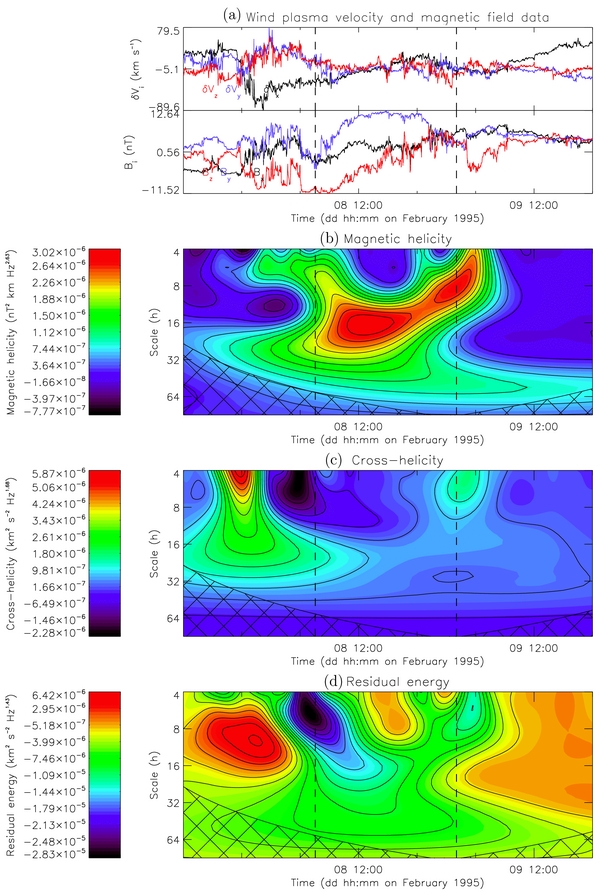
Figure 1. (a) Time profiles of the x, y, and z components (black, blue, and red curves, respectively) of the plasma velocity fluctuations and the magnetic field (in GSE coordinates), acquired by the Wind/SWE and Wind/MFI instruments, respectively, during the transit of the flux rope across the spacecraft on 1995 February 8 (the event is identified by the vertical dashed lines; Feng et al. 2007). (b) Magnetic helicity, (c) cross-helicity, and (d) residual energy adjusted spectrograms as obtained via Equations (14), (16), and (17), respectively, using the Paul mother wavelet; the continuous lines in the bottom panels are the Cones of Influence (COI) and delimit cross-hatched areas where the estimations of  , Hc, and Er are not truly reliable.
Download figure:
Standard image High-resolution imageA smooth clockwise rotation of the magnetic field components (i.e., Hm > 0) is observed at a timescale of about 20 hr, when the event took place, as clearly shown by the portion of the signal within the vertical dashed lines in Figure 1. Magnetic fluctuations superimposed on the large-scale flux rope have amplitudes lower than the ones detected in the preceding time period, that is, in the upstream region, while after the helical structure, that is, in the downstream region, both the plasma velocity and the magnetic field fluctuations tend to be smoothed out. Hence, the flux rope seems to separate two different wind streams characterized by different levels of magnetic field and plasma velocity fluctuations, as also displayed in Figures 1(c) and (d) on the left side of the flux rope, which might indicate the possible role of magnetic turbulence cascade in the dynamical generation process on MHD scales.
The flux rope is clearly identified in the adjusted spectrogram of the magnetic helicity as a right-handed magnetic helical structure with a high helicity, at scales ranging from about 11 to 23 hr (Figure 1(b)): within the flux rope, neither smaller nor larger scales are characterized by helical properties, thus indicating a fairly uniform twisting of the rope magnetic field lines. However, tails of positive magnetic helicity protrude at smaller scales into the upstream regions and, even more, into the downstream regions. These minor helical structures might be ascribed to confined regions of enhanced magnetic field fluctuations, located at the border between the flux rope and the upstream region, that might suggest a local generation of the flux rope via an inverse cascade of magnetic helicity in the turbulent MHD environment (Frisch et al. 1975). The dynamic evolution of incompressible MHD toward a minimum energy state can be characterized by a decay toward a force-free state with zero cross-helicity (Ting et al. 1986; Carbone & Veltri 1992). The flux rope of 1995 February 8 behaves as a typical force-free structure, characterized by σm ∼ 1, and exhibits at the same time a close to zero cross-helicity (Figure 1(c)), as predicted by the solutions of the ideal MHD equations in the framework of a force-free field model (Taylor 1974). These results indicate that the structure might emerge from the MHD decay. However, some few words of caution are necessary concerning the force-free structures. There is indeed no evident reason for the force-free states to be characterized by a close to zero cross-helicity, apart, as discussed above, for the case of MHD decay. Hence, as already suggested by the presence of the smaller-scale helicity structure in the upstream region, the generation of the flux rope of 1995 February 8 might be due to relaxation processes of the magnetic helicity, that is, to a dynamical evolution of the MHD toward a state of maximal magnetic helicity, say a force-free state, and zero cross-helicity. On the contrary, the upstream plasma is characterized by outwardly oriented Alfv nic magnetic fluctuations (of larger amplitude compared to the flux rope) that are positively correlated with the velocity fluctuations. In addition, the residual energy within the flux rope is highly negative (Figure 1(d)), thus pointing, as expected, to a magnetic energy dominance, which, however, extends also to smaller scales in the downstream and, particularly, in the upstream regions, is coincident with the positive helicity tails protruding from the major helical structure. It is worth noting that a similar flux rope (which occurred on 1998 March 28) was already studied by Telloni et al. (2012), thus indicating that such interplanetary objects can be classified on the basis of the characteristics of the MHD invariants of magnetic fluctuations within both the flux rope and the surrounding plasma regions.
The temporal evolution of the average non-normalized and normalized MHD quantities on scales characteristic of the flux rope, that is, on scales corresponding to its energy content, i.e., 11–23 hr, is displayed in the bottom two panels of Figure 2. This figure shows, from top to bottom, the time trends of the components of the plasma velocity, the magnetic field fluctuations, the proton density and temperature, and the plasma β (i.e., the ratio of the plasma to the magnetic pressure). The sixth panel shows the time profiles of  , Hc, and Er, averaged over all the scales within 11–23 hr and normalized to the minimum and maximum values of the corresponding spectrograms.

Figure 2. From top to bottom: time profiles of the x, y, and z components (black, blue, and red curves, respectively) of the plasma velocity fluctuations and the magnetic field in GSE coordinates for the flux-rope event that occurred on 1995 February 8; time profiles of the proton density and temperature, the plasma β; time profiles of  , Hc, and Er (black, blue, and red curves, respectively) averaged over 11–23 hr timescales and normalized with respect to the minimum and maximum values of the corresponding spectrograms; time profiles of
  , σc, and σr (black, blue, and red curves, respectively) averaged over 11–23 hr timescales; the legend lists the mean values of the normalized MHD quantities within the flux rope. Plasma and magnetic data come from the Wind 1 minute database.
Download figure:
Standard image High-resolution imageA typical signature of the flux ropes is a plasma β value significantly lower than the values found in the surrounding medium. This result is clearly evident for the event of 1995 February 8 in the fifth panel of Figure 2, where the plasma β abruptly decreases at the leading edge of the flux rope, that is, at the border separating the two different solar wind streams. The plasma β remains pretty low within the event and slightly increases afterward in the downstream region, even if on the basis of these considerations the flux rope should begin and end earlier. On the other hand, the other plasma parameters, i.e., the proton density and temperature, undergo a sharp decrease across the plasma interface and than exhibit quite constant trends within the event and in the downstream region (although fluctuating a lot), hence suggesting once more a local generation of the flux rope. The normalized MHD quantities displayed in the bottom panel of Figure 2 clearly show the constant α force-free magnetic configuration of the flux rope,  within the event, and that the structure might emerge from the MHD turbulent decay, where also σc ∼ 0. Quite interestingly, although the flux rope and the downstream plasma share approximately the same low level of cross-helicity (sixth panel of Figure 2), the normalized quantity increases moving farther out from the flux rope into the downstream region, thus indicating that the flux rope carries a larger amount of total energy compared to that stored in the downstream plasma. Finally, as expected, the Alfv
 nic MHD fluctuations observed within the upstream region (Figure 1(c)) are characterized by energy equipartition (the red line in the bottom panel of Figure 2).
However, even though many flux ropes from the extended catalog of Feng et al. (2007) look similar to the ones shown in Figures 1 and 2, many other events look different. A typical example of a flux rope with both high magnetic and cross-helicity is displayed in Figures 3 and 4. These data refer to a small structure spotted by Feng et al. (2007) that occurred on 1997 May 9 and was associated with a smooth rotation of the magnetic field vector over a time period of about 4 hr.
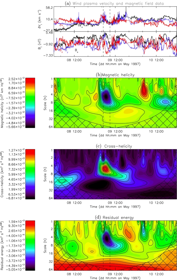
Figure 3. Same as Figure 1, but for the flux-rope event that occurred on 1997 May 9.
Download figure:
Standard image High-resolution image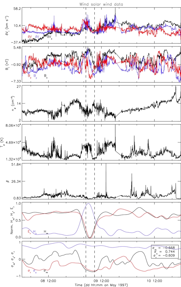
Figure 4. Same as Figure 2, but for the flux-rope event that occurred on 1997 May 9.
Download figure:
Standard image High-resolution imageThe adjusted wavelet spectrograms of the MHD quantities in Figure 3 exhibit a well-localized spot in time and scale for  , Hc, and Er, which indicates that the left-handed helical structure is characterized by both high magnetic helicity (
 ) and cross-helicity (σc ∼ 0.74), and shows as well a clear magnetic energy excess, on a range of scales spanning from about 3 to 8 hr. At odds with the flux rope of 1995 February 8, this helical structure seems to be strictly limited to the time interval when the event took place: its magnetic and cross-helicity are indeed not connected to the surrounding medium. This evidence supports a scenario in which turbulent reconnection leads to the generation of larger-scale magnetic structures; turbulent reconnection is the likely mechanism underlying the flux rope formation. The high cross-helicity is probably due to the rather large amplitude of the components of the plasma velocity fluctuations present during the time interval containing the flux rope (top panel of Figure 3(a)). Thus, computing the average values of the MHD invariants in the 3–8 hr scale band, a strong and well-localized anti-correlation between the magnetic and the cross-helicity within the flux rope is clearly seen. Interestingly, in the bottom panel of Figure 4, the normalized cross-helicity, σc (the blue line), remains roughly constant around a value of 0.7 for the whole observational time period. This result suggests, by comparing this trend with the one shown for the non-normalized quantity, Hc, which is sharply peaked around the +1 value within the flux rope, that the surrounding medium exhibits a lower level of total energy with respect to the energy contained in the flux rope. As usual, the flux rope has a very low value for the plasma β. The levels of the magnetic fluctuations and the fluctuations of the plasma parameters and the MHD invariants in the upstream and downstream plasma regions look very similar (Figure 4), therefore the structure seems to be embedded in the same Alfv
 nic stream, probably generated locally via turbulent reconnection.
4. DISCUSSION
This analysis of flux ropes has been extended to more than 60 events identified in the Wind data by Feng et al. (2007) in order to characterize these events in terms of the MHD invariants of the embedded magnetic fluctuations, with the final goal of relating the differences in the MHD configurations of the helical structures with their different origins either at the Sun or in interplanetary space. The length size of the selected events is of the order of 0.01 AU, with their time duration ranging from tens of minutes to several hours. The mean values of  and |σc|, inferred within the flux ropes and at the characteristic scales corresponding to their energy content, are shown in the scatter plot of Figure 5.

Figure 5. Scatter plot of the absolute values of the normalized magnetic  and cross-helicity |σc|, inferred within the flux ropes identified by Feng et al. (2007) in the Wind data over the 1995–1997 period. Black, green, and red circles refer to events with time durations of Δt ⩽ 2 hr, 2 hr <Δt < 10 hr, and Δt ⩾ 10 hr, respectively. Full and open circles indicate flux ropes approximated by a force-free magnetic configuration with a likelihood of χ2≶0.2, respectively. The dashed line represents the extent of a unit radius, that is, a curve where
  . The dotted and dot–dashed lines indicate the half planes |σc| > 0.45 and
  , respectively.
Download figure:
Standard image High-resolution image
The events were first divided by their time duration Δt into three categories (Δt ⩽ 2 hr, 2 hr <Δt < 10 hr, and Δt ⩾ 10 hr) in order to clarify whether this division by time might be a discriminant for their origin. All of the events analyzed have been displayed in the  –|σc| plane (Figure 5), in order to detect possible clusters of the events in specific regions of the plane. The analysis of flux ropes of different time durations via the rugged invariants of the ideal MHD equations has highlighted that all the events, regardless of their typical timescale, are characterized by a broad range of values of the MHD invariants. Although the magnetic helicity remains rather high (
![$|\sigma _{m}^{r}|\in [0.6:1]$](https://content.cld.iop.org/journals/0004-637X/776/1/3/revision1/apj481506ieqn34.gif) ) within all the flux ropes analyzed (as expected, owing to the large amplitude rotations of the magnetic field components in a flux-rope event), each structure presents variations in the velocity field so significant that σc fluctuates within a broad range of values, i.e., between 0 and ∼0.8 (two flux ropes of the sample even have
) within all the flux ropes analyzed (as expected, owing to the large amplitude rotations of the magnetic field components in a flux-rope event), each structure presents variations in the velocity field so significant that σc fluctuates within a broad range of values, i.e., between 0 and ∼0.8 (two flux ropes of the sample even have  and are above the dot-dashed line in Figure 5). However, these variations are not independent of the magnetic helicity content of the structure. Indeed, interestingly, flux ropes with a given magnetic helicity content are not observed to be characterized by arbitrary values of cross-helicity; rather, it seems that a sort of constraint appears to exist between the two normalized MHD invariants observed within the flux ropes, leading them to distribute, within the uncertainties, along the curve where
  (dashed line in Figure 5). It is worth noting that all three populations tend to cluster along this theoretical curve, and that their distribution is totally independent of their time duration. Furthermore, despite the fact that the analysis is carried out only on the scales of the energy content of the flux ropes, Figure 5 is neither trivial nor automatic. While it is possible to explain why flux ropes with
  have a cross-helicity content close to zero, once one supposes, as discussed above, that the MHD dynamical evolution of the solar wind is based on the generation of the flux ropes themselves, it is much more difficult to theoretically interpret the distribution of the normalized MHD invariants when σc strongly deviates from zero. It is still an open question why, at a given
  the flux ropes seem to be constrained to assume
  , instead of assuming an arbitrary value spanning the 0–1 range. Notwithstanding, in spite of the fact that force-free states do not necessarily imply zero cross-helicity, those flux ropes characterized by a strong signature of cross-helicity have larger reduced χ2 values when they are fit with Bessel functions on the basis of a constant α force-free model. This observational evidence points to a departure from a pure force-free configuration for those flux ropes with high cross-helicity (and lower magnetic helicity). In particular, in the half plane |σc| > 0.45 (indicated by the dotted line in Figure 5), 56% flux ropes are characterized by a χ2 value larger than 0.2, while in the half plane |σc| < 0.45, only 20% of flux ropes have a similar χ2 value. It is significant that not all of the events studied can be well described in the framework of a constant α force-free magnetic field model and that those events that depart from such a configuration have a cross-helicity content highly deviating from a value close to zero. Perhaps two populations of flux ropes exist: one emerging locally from the MHD decay, and thus characterized by a maximal magnetic helicity and close-to-zero cross-helicity, which can be well described as force-free structures, the other originating either on the Sun or in interplanetary space, characterized by both high magnetic and cross-helicity, which sometimes cannot be well approximated by a force-free magnetic field state. In fact, non-force-free models have also been developed to reproduce observations (Dasso et al. 2005). It is clear that this issue cannot be fully proved only on the basis of the observational evidence presented in this study; further investigations are still required.
As a matter of fact, besides solutions with a maximal magnetic helicity and zero cross-helicity (belonging more to laboratory plasma) and, vice versa, with maximal cross-helicity and zero magnetic helicity (typical of free space plasma), MHD equations also predict a third state (Ting et al. 1986; Carbone & Veltri 1992). In this third state, both the magnetic and cross-helicity significantly deviate from zero (Hm≶0 and Hc≶0) and the system is very far from energy equipartition (Er < 0, as for the magnetically dominated flux ropes). The analysis thus seems to indicate that this physical state is actually observed in some of the analyzed flux ropes.
5. CONCLUSIONS
In this paper, an extended analysis was performed of flux-rope events identified by Feng et al. (2007) in the Wind data of the solar wind plasma over the time period 1995 to 1997. The approach used was introduced by Telloni et al. (2012) and is based on the localization of flux ropes both in time and at a given scale range using wavelet spectrograms (see Equations (14)–(19)) for the calculation of the rugged invariants of the ideal MHD equations.
As a first attempt, flux ropes were divided according to their time duration, namely, flux ropes extended for a time period Δt ⩽ 2 hr, flux ropes marked by 2 hr <Δt < 10 hr, and flux ropes lasting for Δt ⩾ 10 hr. However, statistical analysis has shown that regardless of their time duration, all of the flux ropes show a plasma β much lower than the surrounding environment and a rather high level of reduced normalized magnetic helicity, i.e.,  . On the contrary, the other MHD invariant, the normalized cross-helicity, varies within a broad range of values, that is 0 ⩽ |σc| ⩽ 0.8, although not independently of the magnetic helicity content of the flux rope. The two MHD quantities are somehow constrained to assume, within the flux rope and at the scales corresponding to its energy content, values such that
  . It is worth mentioning that this strong variability of the cross-helicity is caused by the presence of large amplitude plasma velocity fluctuations within the ropes (see, for example, the top panel of Figure 3(a)), although the theoretical aspects underlying the existence of such a constraint between the magnetic and cross-helicity of these kinds of long-lived structures are still to be established.
Furthermore, it has been noted that some flux-rope events seem to be the interfaces between different portions of the solar wind plasma exhibiting different characteristics, as is the case for the flux rope detected on 1995 February 8, which is shown in Figures 1 and 2. In this case, the upstream and downstream regions are characterized by a different level of activity in both magnetic and velocity fluctuations (also recognizable in the spectrograms of the cross-helicity and of the residual energy), as well as in the proton density and temperature. In a very recent paper by Arnold et al. (2013), it was pointed out that regions of interfaces as single, double, or triple current sheets, connecting plasma streams with different properties might support a flux-tube picture of the solar wind, with those tubes originating from the solar surface. However, as discussed in Section 3, the flux rope that occurred on 1995 February 8 exhibits values of the MHD invariants that extend both upstream and downstream of the rope, thus indicating a possible local generation of the magnetic structure. On the other hand, flux ropes with MHD characteristics similar to those shown in Figures 3 and 4 have also been observed in the data set analyzed. In this case, the ropes appear as well localized, isolated magnetic structures embedded in the same solar wind stream as very energetic events at the characteristic scale of the flux rope, and exhibit values of the MHD invariants totally different from those of the upstream and downstream regions.
This work was supported by Italian Space Agency (ASI) grants (I/013/12/0) and by "Borsa Post-doc POR Calabria FSE 2007/2013 Asse IV Capitale Umano—Obiettivo Operativo M. 2."