


ABSTRACT
We study the radial dependence in stellar populations of 33 nearby early-type galaxies with central stellar velocity dispersions σ* ≳ 150 km s−1. We measure stellar population properties in composite spectra, and use ratios of these composites to highlight the largest spectral changes as a function of radius. Based on stellar population modeling, the typical star at 2Re is old (∼10 Gyr), relatively metal-poor ([Fe/H] ≈ −0.5), and α-enhanced ([Mg/Fe] ≈ 0.3). The stars were made rapidly at z ≈ 1.5–2 in shallow potential wells. Declining radial gradients in [C/Fe], which follow [Fe/H], also arise from rapid star formation timescales due to declining carbon yields from low-metallicity massive stars. In contrast, [N/Fe] remains high at large radius. Stars at large radius have different abundance ratio patterns from stars in the center of any present-day galaxy, but are similar to average Milky Way thick disk stars. Our observations are thus consistent with a picture in which the stellar outskirts are built up through minor mergers with disky galaxies whose star formation is truncated early (z ≈ 1.5–2).
1. INTRODUCTION
Galaxies exhibit strong correlations between their mass and their metallicity. It is thought that mass–metallicity correlations arise from star-formation-driven winds preferentially removing metals from low-mass galaxies (e.g., Larson 1974; Dekel & Woo 2003; Tremonti et al. 2004). In the case of elliptical galaxies, the mass–metallicity relation is manifested most strongly in the Mgb–σ* relation (Dressler et al. 1987; Bender et al. 1993). If indeed elliptical galaxies grow through merging, as expected in a hierarchical universe, then naively we have an accounting problem—how to make massive metal-rich galaxies through the addition of smaller metal-poor units (Faber et al. 2007; Naab & Ostriker 2009).
The situation is more nuanced since (1) mass–metallicity relations evolve with cosmic time, meaning that all galaxies had lower metallicities in the past (e.g., Erb et al. 2006; Mannucci et al. 2010) and (2) galaxies have known radial stellar population gradients. In general, the Mgb–σ* relation is measured in the high surface-brightness galaxy center, where the metallicity is highest. A full census of the metallicity and abundance ratio content of elliptical galaxies requires spatially resolved observations. The recent discovery of dramatic (factor of 2–4) size growth in elliptical galaxies from z ≈ 2 to the present (e.g., Daddi et al. 2005; Trujillo et al. 2006; van Dokkum et al. 2008; van der Wel et al. 2008; Cimatti et al. 2008; Damjanov et al. 2009; Williams et al. 2010; Cassata et al. 2010) is now supported by an increasing number of dynamical studies (Cappellari et al. 2009; van de Sande et al. 2011). It seems that much of the late-time growth of elliptical galaxies has occurred in their outer parts (e.g., Naab et al. 2009; van Dokkum et al. 2010). If elliptical galaxies are formed in two phases, with an early rapid gas-rich phase making the central compact galaxy observed at high redshift, and a late-time accretion phase building up the outer parts (e.g., Oser et al. 2010; Hilz et al. 2012, 2013), we might hope to see the imprint of these two phases in the stellar population gradients.
In principle, the stellar outskirts carry important information about the late-time assembly history of elliptical galaxies. In practice, observations of the stellar populations in elliptical galaxy outskirts are challenging, since their surface brightnesses drop steeply with radius. Despite more than 30 yr of effort, most observations of stellar population gradients do not extend much beyond the half-light radius (Spinrad & Taylor 1971; Faber et al. 1977; Gorgas et al. 1990; Fisher et al. 1995; Kobayashi & Arimoto 1999; Ogando et al. 2005; Brough et al. 2007; Baes et al. 2007; Annibali et al. 2007; Sánchez-Blázquez et al. 2007; Rawle et al. 2008; Kuntschner et al. 2010; Coccato et al. 2010, 2011). While integral-field spectrographs have brought a golden age in the study of spatially resolved galaxy properties (Emsellem et al. 2004; Sarzi et al. 2006; Cappellari et al. 2006, 2012), there are still few observations that extend beyond the half-light radius in integrated light (Carollo et al. 1993; Carollo & Danziger 1994; Mehlert et al. 2003; Kelson et al. 2006; Weijmans et al. 2009; Spolaor et al. 2010; Pu et al. 2010; Pu & Han 2011). To our knowledge, there are fewer than 30 integrated-light observations in total (using different instruments and techniques) that reach beyond Re in massive elliptical galaxies in the literature. There are also a handful of studies that reach into elliptical galaxy halos using resolved stellar population studies (e.g., Kalirai et al. 2006; Harris et al. 1999; Rejkuba et al. 2005; Harris et al. 2007; Crnojević et al. 2013). We thus present the largest and most homogeneous spectroscopic sample to date of observations ≳ 2Re.
Specifically, building on the preliminary study of Greene et al. (2012, Paper I, hereafter), we use integral-field observations taken with the Mitchell Spectrograph at McDonald Observatory. We measure robust stellar population gradients out to 2.5Re in massive local elliptical galaxies. With a 107'' × 107 '' field of view, the Mitchell spectrograph is uniquely suited to explore massive galaxy halos. Our sample comprises 33 galaxies, 8 of which were already presented in Paper I.
We present the sample in Section 2, the observations and data reduction in Section 3, our analysis in Section 4, and the radial variations in stellar populations in Section 5. We discuss our findings in the context of the hierarchical assembly of massive galaxies in Section 6, and summarize in Section 7.
2. SAMPLE
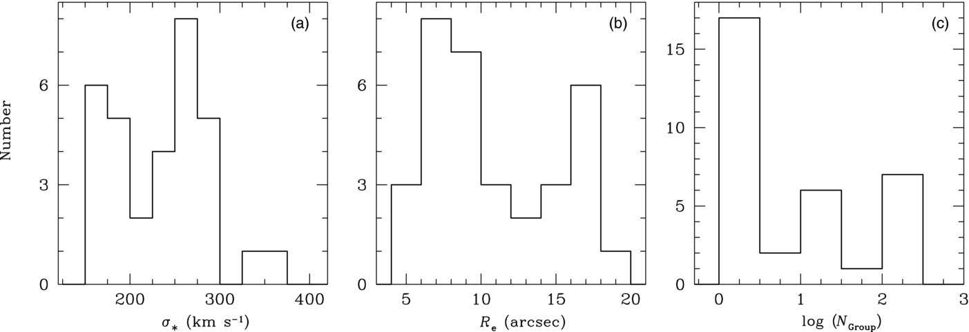
We select our sample of massive early-type galaxies from the Sloan Digital Sky Survey (SDSS; York et al. 2000). The spectral resolution of the Mitchell Spectrograph is σinst ≈ 150 km s−1 at 4700 Å; we select galaxies with dispersion measurements from the SDSS that are greater than this value. Individual fibers are 4'' in diameter, and so we aim for galaxies with effective radii at least twice as large. Galaxies with distances of 40–95 Mpc are large enough to be well-resolved but small enough to fit into one pointing. We use a color selection of u − r > 2.2 (Strateva et al. 2001), which preferentially selects early-type galaxies, and then remove the few edge-on disk galaxies by hand. There is no clean way to remove S0s; we keep them in the sample and eventually hope to use kinematic information to cleanly identify them. For now, we note the photometrically classified S0 galaxies from the RC3 (de Vaucouleurs et al. 1991) in Table 1, where we list the full galaxy sample. Finally, we use the group catalogs of Yang et al. (2007), Zhu et al. (2010), and Wetzel et al. (2012) to get a global estimate of the galaxy environment. We show the full distribution of σ*, half-light radius, and group membership for each galaxy in the sample in Figure 1.

Figure 1. (a) Distribution of central σ* (km s−1) as measured by the SDSS for the entire sample presented in this paper. (b) Distribution in effective radius (''). At the typical distance (∼70 Mpc) of our sample, 8'' ≈ 2.5 kpc. (c) Distribution of the log of the number of group members for each galaxy (Yang et al. 2007; Zhu et al. 2010; Wetzel et al. 2012). Note that this is a global measurement of environment.
Download figure:
Standard image High-resolution imageTable 1. The Sample
| Galaxy | R.A. | Decl. | z | mg | Re | σ* | te | SB | Nf | Env. |
|---|---|---|---|---|---|---|---|---|---|---|
| (1) | (2) | (3) | (4) | (5) | (6) | (7) | (8) | (9) | (10) | (11) |
| NGC 219 | 00:42:11.3 | +00:54:16.3 | 0.018 | 13.4 | 4.4 | 184 | 120 | 21.9 | 5 | F |
| NGC 426 | 01:12:48.6 | −00:17:24.6 | 0.018 | 13.1 | 8.3 | 285 | 120 | 21.9 | 8 | F |
| NGC 474a | 01:20:06.6 | +03:24:55.8 | 0.008 | 12.4 | 18.1 | 163 | 120 | 22.0 | 96 | F |
| CGCG 390−096 | 03:30:17.1 | −00:55:12.6 | 0.021 | 13.6 | 7.8 | 204 | 120 | 23.4 | 18 | F |
| NGC 661 | 01:44:14.6 | +28:42:21.1 | 0.013 | 14.4 | 19.9 | 190 | 120 | 22.8 | 18 | G |
| NGC 677 | 01:49:14.0 | +13:03:19.1 | 0.017 | 12.9 | 9.6 | 257 | 160 | 22.0 | 25 | G |
| UGC 1382 | 01:54:41.0 | −00:08:36.0 | 0.019 | 13.2 | 9.9 | 195 | 120 | 22.6 | 30 | F |
| NGC 774a | 01:59:34.7 | +14:00:29.5 | 0.015 | 13.0 | 20.9 | 165 | 120 | 24.0 | 111 | F |
| IC 301 | 03:14:47.7 | +42:13:21.6 | 0.016 | 13.1 | 12.6 | 159 | 120 | 22.7 | 38 | C |
| NGC 1286a | 03:17:48.5 | −07:37:00.6 | 0.014 | 13.2 | 18.1 | 163 | 180 | 24.4 | 103 | F |
| IC 312 | 03:18:08.4 | +41:45:15.6 | 0.017 | 13.3 | 18.1 | 218 | 120 | 24.8 | 48 | C |
| NGC 1267 | 03:18:44.7 | +41:28:02.8 | 0.018 | 13.3 | 6.4 | 236 | 120 | 22.1 | 7 | C |
| NGC 1270 | 03:18:58.1 | +41:28:12.4 | 0.017 | 13.1 | 6.4 | 373 | 120 | 21.3 | 11 | C |
| NVSS J0320+4136 | 03:20:50.7 | +41:36:01.5 | 0.018 | 13.4 | 4.5 | 274 | 120 | 21.7 | 8 | C |
| UGC 4051 | 07:51:17.6 | +50:10:45.4 | 0.021 | 13.1 | 8.6 | 300 | 180 | 22.3 | 14 | G |
| NGC 3837 | 11:43:56.4 | +19:53:40.4 | 0.021 | 13.1 | 8.1 | 265 | 120 | 22.2 | 20 | C |
| NGC 3842 | 11:44:02.1 | +19:56:59.3 | 0.021 | 12.7 | 20.5 | 284 | 120 | 22.8 | 99 | C |
| NGC 4065 | 12:04:06.1 | +20:14:06.2 | 0.021 | 12.9 | 12.5 | 278 | 120 | 22.4 | 38 | C |
| IC 834 | 12:56:18.5 | +26:21:32.0 | 0.021 | 13.3 | 7.3 | 255 | 120 | 21.9 | 12 | F |
| NGC 4908 | 13:00:54.4 | +28:00:27.4 | 0.017 | 13.1 | 18.5 | 236 | 120 | 23.8 | 74 | F |
| NGC 4952 | 13:04:58.3 | +29:07:20.0 | 0.020 | 12.9 | 12.1 | 292 | 120 | 22.5 | 34 | F |
| NGC 5080 | 13:19:19.2 | +08:25:44.9 | 0.022 | 13.0 | 7.8 | 269 | 120 | 21.7 | 17 | F |
| NGC 5127 | 13:23:45.0 | +31:33:57.0 | 0.016 | 12.8 | 22.9 | 275 | 120 | 23.9 | 111 | F |
| NGC 5423a | 14:02:48.6 | +09:20:29.0 | 0.020 | 12.9 | 10.9 | 263 | 120 | 22.9 | 34 | G |
| NGC 5982 | 15:38:39.8 | +59:21:21.0 | 0.010 | 11.8 | 17.9 | 239 | 120 | 22.3 | 40 | F |
| IC 1152 | 15:56:43.3 | +48:05:42.0 | 0.020 | 13.0 | 7.7 | 258 | 120 | 22.1 | 14 | G |
| IC 1153a | 15:57:03.0 | +48:10:06.1 | 0.020 | 13.0 | 9.8 | 241 | 120 | 22.0 | 21 | G |
| CGCG 137−019 | 16:02:30.4 | +21:07:14.5 | 0.015 | 13.1 | 8.7 | 174 | 120 | 22.5 | 22 | F |
| NGC 6127 | 16:19:11.5 | +57:59:02.8 | 0.016 | 13.8 | 11.2 | 247 | 120 | 22.5 | 24 | F |
| NGC 6482 | 17:51:48.8 | +23:04:19.0 | 0.013 | 12.4* | 9.7 | 292 | 120 | 22.5 | 90 | G |
| NGC 6964 | 20:47:24.3 | +00:18:02.9 | 0.013 | 12.9 | 17.0 | 188 | 120 | 23.6 | 73 | G |
| NGC 7509 | 23:12:21.4 | +14:36:33.8 | 0.016 | 13.1 | 9.0 | ... | 180 | 22.3 | 28 | F |
| NGC 7684a | 23:30:32.0 | +00:04:51.8 | 0.017 | 13.0 | 15.8 | 169 | 240 | 22.2 | 36 | F |
Notes. Column 1: galaxy name. We indicate as a known S0 galaxies from RC3 (de Vaucouleurs et al. 1991). Column 2: R.A. (hr) in J2000. Column 3: Decl. (deg) in J2000. Column 4: redshift from the SDSS. Column 5: g-band model magnitude (mag) from the SDSS. NGC 6482 is not in the SDSS, and here we list the B-band magnitude (total) from RC3 (de Vaucouleurs et al. 1991). Column 6: major axis half-light radius ('') as measured by the SDSS. Column 7: stellar velocity dispersion (km s−1) as measured by the SDSS. We tabulate the SDSS values here since the sample was selected based on these values. Column 8: exposure time (minutes). Column 9: surface brightness at 2Re in r-band (mag arcsec−2). Column 10: number of fibers included in the 1.5–2Re bin. Column 11: we sort galaxies into "F"ield, "G"roup, and "C"luster based on the number of group members from the Yang et al. (2007) catalog (see also Zhu et al. 2010; Wetzel et al. 2012). Field galaxies have Ngroup < 5, group indicates 5 < Ngroup < 50, and cluster indicates richer than 50 group members. The grouping is indicative only. We note that the Perseus cluster is not included in these group catalogs, but is well-represented in our sample.
Download table as: ASCIITypeset image
3. OBSERVATIONS AND DATA REDUCTION
The new observations of 25 galaxies presented in this paper were observed over three runs in 2012 January 17–20, May 20–24, and October 15–18. We include here also the eight galaxies presented in Greene et al. (2012), for a total sample of 33 galaxies. The observations were made with the George and Cynthia Mitchell Spectrograph (the Mitchell Spectrograph, formerly VIRUS-P; Hill et al. 2008) on the 2.7 m Harlan J. Smith telescope at McDonald Observatory. The Mitchell Spectrograph is an integral-field spectrograph composed of 246 fibers covering a 107'' × 107'' field of view with a one-third filling factor. Each of the 246 fibers subtends 4 2 and they are assembled in an array similar to Densepak (Barden et al. 1998). The Mitchell Spectrograph has performed a very successful search for Lyα emitters (Adams et al. 2011; Finkelstein et al. 2011; Blanc et al. 2011) and has become a highly productive tool to study spatially resolved kinematics and stellar populations in nearby galaxies (Blanc et al. 2009; Yoachim et al. 2010; Murphy et al. 2011; Adams et al. 2012).
We use the low-resolution (R ≈ 850) blue setting of the Mitchell Spectrograph. Our wavelength range spans 3550–5850 Å with an average spectral resolution of 5 Å FWHM. This resolution delivers a dispersion of ∼1.1 Å pixel−1 and corresponds to σ* ≈ 150 km s−1 at 4300 Å, our bluest Lick index. Each galaxy was observed for a total of ∼2 hr on source with one-third of the time spent at each of three dither positions to fill the field of view. Initial data reduction is accomplished using the custom code Vaccine (Adams et al. 2011; Murphy et al. 2011). The details of our data reduction are described in Greene et al. (2012) and Murphy et al. (2011), so we repeat only a brief overview for completeness here.
Initial overscan and bias subtraction are performed first on all science and calibration frames. Twilight flats are used to construct a trace for each fiber, which takes into account curvature in the spatial direction, following Kelson (2003) to avoid interpolation and thus correlated errors. A wavelength solution is derived for each fiber based on arcs taken both at the start and end of the night using a fourth-order polynomial. The typical residual variations about this best-fit fourth-order polynomial are between 0.05 and 0.1 Å depending on the night. The flat field is constructed from twilight flats, with the solar spectrum modeled and removed. The flat field is stable to <0.1 pixel for typical thermal variations in the instrument of less than 5°C. When the temperature variation exceeded 5°C over a night, the reductions are split, with the nearest calibration frame in temperature being used. The flat field is then applied to all of the science frames, and corrects variations in the individual pixel response, in the relative fiber-to-fiber variation, and in the cross-dispersion profile shape for every fiber.
The sky is modeled using off-galaxy sky frames observed with a sky-object-object-sky pattern, with 10 minute exposure times on sky and 20 minute object exposures. The sky nods are processed in the same manner as the science frames described above. In general, each sky nod is weighted equally, although in unstable conditions (clouds, for instance) we experiment with different weighting schemes to achieve an optimal sky subtraction. Since the galaxies are fainter than the sky in their outskirts, sky subtraction is a limiting factor for us. We quantify our uncertainties due to sky subtraction in Section 4.1.1. Finally, cosmic rays are identified and masked.
We use software developed for the VENGA project (Blanc et al. 2009, 2013) for flux calibration and final processing. We observe flux calibration stars each night using a six-point dither pattern and derive a relative flux calibration in the standard way. Then we use tools developed by M. Song et al. (in preparation) to derive an absolute flux calibration relative to the SDSS imaging. Synthetic photometry is used to scale the spectra to match the SDSS g-band image of each field. Finally, all fibers are interpolated onto the same wavelength scale and combined.
Since most of our galaxies have SDSS spectra, we can test the wavelength dependence of the flux calibration by comparing the shape of the spectrum in the central fiber of the Mitchell Spectrograph with the SDSS spectrum. We find ≲ 5% agreement in nearly all cases, with no more than ∼10% differences at worst.
3.1. Effective Radii
In Paper I we adopted the SDSS model radius (the de Vaucouleurs fit) as the effective radius (Re). While there is considerable evidence that the shape of the light profile changes systematically with galaxy mass (e.g., Caon et al. 1993; Kormendy et al. 2009), fitting the galaxies with a fixed Sérsic index of four has the benefit that we are less sensitive to both sky subtraction errors (Mandelbaum et al. 2005; Bernardi et al. 2007) and to the detailed shape of the light profile in the very faint wings (e.g., Lackner & Gunn 2012). In the effort to have a uniform analysis, we have therefore adopted the effective radii published by the SDSS. The galaxy NGC 6482 is not in the SDSS, and we have adopted Re from NED in this case. Below we will examine bins in physical as well as Re-scaled radii to mitigate uncertainties in the measurement and meaning of Re (e.g., Kormendy et al. 2009; Huang et al. 2013a).
3.2. Radial Bins
Individual spectra, with the exception of those at the very center of the IFU, have inadequate signal for stellar population analysis. Therefore, all of our analysis is performed on binned spectra. We utilize four binning schemes here, in all cases defining elliptical annuli based on the axis ratio measured by the SDSS. First, for the maximum spatial resolution, we create bins with radial width of 4'', the width of an individual fiber. Second, we make bins of width 0.5Re. In Paper I, these two binning schemes were nearly identical, given that most of the galaxies had effective radii of ∼8''. However, in our larger sample, many of the galaxies have effective radii of 10''–25'', requiring a finer binning scheme. In the end, our highest spatial resolution corresponds to 0.2–0.5Re depending on the galaxy. Third, we make bins of width Re, from which we measure σ*. Fourth, we make bins with fixed physical sizes of 0–15 kpc in 3 kpc increments. For reference, in Table 1 we include the number of spectra that are combined in the 1.5–2Re bin, and the surface brightness of each galaxy at 2Re. We typically achieve a signal-to-noise ratio (S/N) of >30 per pixel at a surface brightness brighter than r < 23 mag arcsec−2.
4. ANALYSIS
As discussed in detail in Paper I, we will use Lick indices as a tool to trace the stellar populations, rather than full spectral synthesis models, given both the imperfect flux calibration of our data and the difficulty in modeling the effects of abundance ratio changes (e.g., Worthey et al. 1994) self-consistently (e.g., Gallazzi et al. 2005). In addition, we construct coadded spectra to increase the contrast in percent-level variations around absorption features of interest.
4.1. Equivalent Widths, Emission Line Corrections, and Stellar Population Modeling
As in Greene et al. (2012), we use lick_ew (Graves & Schiavon 2008) to measure the Lick indices. First, however, we must correct for low-level emission that can fill in the absorption lines and artificially lower their equivalent widths (EWs). Low-EW emission from warm ionized gas is very common in the centers of elliptical galaxies (Sarzi et al. 2010; Yan & Blanton 2012). In particular, the emission from Hβ is weak in all cases, but even a 0.1 Å error in the Hβ EW can lead to errors of ∼2 Gyr in the modeling (e.g., Schiavon 2007).
In Paper I, we utilized pPXF+GANDALF developed by M. Sarzi (Sarzi et al. 2006) and M. Cappellari (Cappellari & Emsellem 2004) to simultaneously model the stellar absorption and emission lines. Here, instead, we fit each spectrum with an empirical template drawn from the composite spectra of Graves et al. (2010). We then fit the [O iii] emission in the residual spectrum, and subtract both [O iii] and Hβ, assuming that the Hβ emission is 70% of the [O iii] flux (good to within a factor of two, Trager et al. 2000b; Graves et al. 2007). In addition, we fit Gaussians to residuals around strong sky lines at 5200 and 5460 Å, and subtract them.
The strongest emission (≳ 0.2 Å in more than one radial bin) is found in NGC 426, NGC 661, NGC 677, NGC 7509, NGC 7684, and UGC 1382. We found that our GANDALF results were sensitive to template mismatch, and so adopted this iterative approach that gives us more control over the templates but less control over the line strengths. The results are reasonably consistent between the two techniques for sources with Hβ > 0.1 Å in the GANDALF fits: 75% of these are detected in our iterative method, which returns Hβ EWs that are ∼60% weaker than those derived from GANDALF. In the future our goal is to refine the GANDALF measurements using models with a range in [α/Fe] (e.g., Coelho et al. 2007; Vazdekis et al. 2010; Conroy et al. 2013).
We then use lick_ew (Graves & Schiavon 2008) on the emission-line-corrected spectra. This code corrects for both the instrumental and intrinsic velocity dispersion, the latter measured using pPXF. The indices are put onto a modified Lick system presented by Schiavon (2007) based on flux-calibrated spectra. In order to demonstrate that we are on the same system, we compare the Lick indices from the flux-calibrated SDSS spectra (the inner 3'') with those from the central 4'' fiber in our data, but we exclude NGC 219, NGC 426, NGC 677, NGC 1267, and IC 301 from the comparison due to the presence of bright stars near the nucleus. There is no net offset between the two sets of indices in any case, with 〈(EWMS − EWS)/EWS〉 = 0.01 ± 0.09. Hβ and 〈Fe〉 each have a scatter of ∼10% while Mgb and the G-band each have a scatter of ∼5%.
As in Paper I, we use the stellar population modeling code EZ_Ages (Graves & Schiavon 2008) to convert the Lick indices from the composite spectra to physical parameters (age, [Fe/H], [α/Fe]). The code works on a hierarchy of index pairs, starting with Hβ and 〈Fe〉, and iteratively solves for the age, abundance and abundance ratios. The models of Schiavon (2007) include abundance ratio differences using the methodology of Trager et al. (2000b) and the response functions of Korn et al. (2005). In our default runs, we utilize the α-enhanced isochrone from Salasnich et al. (2000) and the default assumption that [O/Fe] = 0.5. We revisit this final assumption in Section 6.1.
4.1.1. Uncertainties
Our error budget is dominated by small errors in sky subtraction, particularly when sky lines fall within the bands of the Lick index measurements. Thus, for each extracted spectrum, we generate eight perturbed spectra with the fiducial sky subtraction scaled by ±5%, 4%, 3%, 2% respectively. We then run our entire procedure on these perturbed spectra. The final errors represent the spread in EWs produced by these variations in sky subtraction. As described in Paper I, our sky subtraction uncertainty is unlikely to exceed 3%, so these error bars are conservative.
In Paper I, all of our targeted galaxies had similar sizes and distances. Therefore, at a given radial distance, we achieved similar quality spectra for all galaxies. In this sample we span a much wider range in galaxy stellar mass, and reach our limiting surface brightness at different radii for each galaxy. At a certain point, the Lick index measurements are no longer reliable. To ensure some consistency across all galaxies, we do not consider lick index measurements from spectra with S/N per pixel ⩽20.
4.2. Composite Spectra
While measuring Lick indices is a very powerful technique at high S/N, at the large radii that we are working systematic effects such as small errors in sky subtraction and flux calibration can cause large uncertainties in the Lick indices measured from individual objects. With our sample size, we benefit from averaging over multiple galaxies at each radial bin. The composite spectra will suffer less from the vagaries of sky subtraction and flux calibration, which occur at different wavelengths in each galaxy rest-frame (e.g., Graves et al. 2009; Yan 2011). We are able to examine radial variations in the composite spectra at the percent level.
We first divide the galaxies into three bins of central σ* of 150 < σ* < 200, 200 < σ* < 250, and 250 < σ* < 300 km s−1, since we know that the stellar population properties are a strong function of σ* (e.g., Worthey et al. 1992; Bender et al. 1993; Trager et al. 2000a; Graves et al. 2009). Note that the bins would not change if we used σ* within Re, but that in this way our bins are more consistent with the large literature based on the SDSS measurements. We combine spectra that have already been emission-line-corrected. We interpolate the rest-frame spectra onto the same wavelength grid and then smooth each galaxy to the highest dispersion in the stack (300 km s−1 for the high-dispersion bin and 200 km s−1 for the low-dispersion bin). However, to increase the contrast, we will focus exclusively on the highest- and lowest-dispersion bins here. We remove the continuum by dividing each spectrum by a heavily smoothed version of itself. This step simultaneously normalizes all spectra to the same level and ensures that differences in continuum shape (whether real or due to small errors in sky subtraction or flux calibration) do not impact the final line strengths. We then combine all pixels at each wavelength using the biweight estimator, which should be robust even with limited statistics (Beers et al. 1990). We experiment with multiplying the composite spectrum by the median continuum before measuring indices, but the changes to the Lick indices are negligible in all cases.
The composite spectra are shown in Figure 2. Again we focus only the lowest- and highest-dispersion bins, which contain 11 galaxies each (excluding NGC 219 due to severe night sky contamination and NGC 6482 due to contamination from a neighboring galaxy). The spectra are strikingly similar as a function of radius, so we use ratio spectra to highlight the percent-level radial variations (Figure 2, right). Specifically, we divide each composite spectrum, at each radial position, by the composite spectrum at 0.5–1 Re. We choose this radius, rather than the central bin, because as we will see below the largest variance in spectral properties occurs in the very center. We will examine the radial trends in these spectra in detail in Section 5. For now, we note only that the strongest variations are seen in carbon, Mgb, and perhaps nitrogen.

Figure 2. Left: composite spectra in radial bins of effective radius, from 0.5 to 2.5Re. We have divided the sample into three σ* bins, and show the largest (250 < σ* < 300 km s−1; top five red spectra) and smallest dispersion (150 < σ* ⩽ 200 km s−1; bottom five blue spectra) galaxies here. All spectra have been normalized at 4500 Å, and the offsets shown here are arbitrary. Right: to highlight the differences between spectra in subsequent radial bins, we have divided each spectrum by the second (0.5Re < R < 1Re) bin, shown in the same order as on the left. Again, offsets are arbitrary but dotted lines denote unity, so we are seeing variations at the 1%–5% level in these spectra. Vertical dashed lines highlight spectral bands that show large variations including Fe lines (dotted), molecular bands CN, C2, and MgH (dashed) and Hβ (dot-dashed). The low-σ* galaxies, being fainter, have much lower surface brightness in their outer parts, and thus we only plot the residuals out to 2Re, where we deem our results reliable.
Download figure:
Standard image High-resolution imageTo determine the level of variation in the composite spectra, we generate 100 trial composite spectra by randomly drawing from the total list of galaxies within that σ* bin, with replacement. We measure Lick indices from each of these 100 trial spectra. We then assign errors on the Lick indices measured from the stack derived to enclose 68% of the Lick indices measured from the 100 trials.
5. RADIAL VARIATIONS IN STELLAR POPULATIONS
We have extracted spectra out to 2.5Re for a sample of 33 local massive elliptical galaxies with stellar velocity dispersions ranging from 150 < σ* < 370 km s−1. We use the composite spectra to measure high fidelity radial trends in the stellar population properties, including age, [Fe/H], and detailed abundance ratio gradients. From the gradients, we make inferences about when, where, and how the stars in the outer parts were formed. First, we confirm that we can recover reliable Lick indices from our composite spectra (Section 5.1). Second, we look at the dominant radial trends as revealed in ratios of the composite spectra (Section 5.2). Third, and finally, we present the radial trends in stellar populations (Section 5.3).
5.1. Radial Trends in Lick Indices
We first investigate the average radial profile in the Lick indices as a function of radius in the high-dispersion (250 < σ* < 300 km s−1) and low-dispersion (150 < σ* < 200 km s−1) galaxies. We use Lick indices measured from the composite spectra (Section 4.2) and plot them as filled points as a function of radius in Figure 3. As a check on the composite spectra, we also calculate the median indices at each radius from the individual galaxy measurements, divided into the same high- and low-dispersion groups. These median profiles are shown as lines in Figure 3. The consistency between the composite and median measurements gives us confidence in the measurements from our composite spectra.

Figure 3. We show the median and standard deviation in each index (Mgb, 〈Fe〉, and Hβ) as a function of radius (units of kpc on the left and Re on the right) for low-dispersion (150 < σ* < 200 km s−1; dotted lines) and high-dispersion galaxies (250 < σ* < 300 km s−1; solid lines). Overplotted in points are the measurements from the composite spectra in the high-dispersion (filled circles) and low-dispersion (filled squares) galaxies. We also indicate the typical scales for the central and outer components of galaxies as measured in Huang et al. (2013a; gray vertical dashed lines).
Download figure:
Standard image High-resolution imageWe show radial profiles both as a function of radius scaled to Re and in physical units of kpc. Using bins scaled to the effective radius is convenient when comparing galaxies of varying size. However, there are two problems with using Re-normalized units. First, Re is difficult to measure, and becomes more so for high-mass galaxies that have an extended low surface-brightness halo (e.g., Kormendy et al. 2009). Second, Re grows with cosmic time. Therefore, if we are searching for changes in stellar populations that correspond to different epochs in galaxy growth, we may want to look at physical as well as Re-scaled radii.
Interestingly, most of the variation in the Lick indices occurs within the central ∼7 kpc or ∼1.5Re. From photometric fitting, Huang et al. (2013a, 2013b) find evidence for a distinct outer (∼10 kpc) component, perhaps formed via accretion. We see a tantalizing hint that the index values are converging beyond ≳ 2Re between the low- and high-dispersion galaxies. If indeed the central compact regions of elliptical galaxies were formed in a very rapid event at high redshift, with the outer parts accreted later (e.g., Thomas et al. 2005; Oser et al. 2010), then we might be reaching a radius where a large fraction of the mass has been accreted from smaller galaxies. As our next means of studying radial stellar population trends, we examine the stacked spectra as a function of radius.
5.2. Radial Trends at the Percent Level
In addition to measuring more reliable Lick indices at large radius, we examine percent-level variations directly from the stacked spectra. While we do not derive any quantitative conclusions from this exercise, it is nevertheless revealing to see where the largest radial variance occurs in the spectra. We create composite spectra for two groups of galaxies divided by high (σ* = 250–300 km s−1) and low (σ* = 150–200 km s−1) stellar velocity dispersion, and we add them radially in units of Re (Figure 2) and kpc (Figure 4). Since the largest variations occur within the central bin, we have made ratio spectra (Section 4.2) dividing by the composite spectrum in the 0.5–1Re or the 3–6 kpc bin respectively. "Emission" features in the ratio spectra are manifestations of a declining EW relative to ∼Re, while "absorption" indicates increasing EW.

Figure 4. Ratio spectra as in Figure 2 (right). Here, each radial bin has a fixed physical size of 3 kpc (the five bins range from 0 to 15 kpc) and we show the ratio with the 3–6 kpc bin. We cannot reach further than the 6–9 kpc bin for the low-dispersion stack. Offsets are arbitrary but dotted lines denote unity, so we are seeing variations at the 1%–5% level in these spectra. Vertical dashed lines highlight spectral bands that show large variations including Fe lines (dotted), molecular bands CN, C2, and MgH (dashed) and Hβ (dot-dashed).
Download figure:
Standard image High-resolution imageThe most prominent radial changes are seen in the molecular bands CN (the most prominent band is at 4150 Å), C2 (the Swan band at 4668 Å, and another Swan band at ∼5100 Å on the wing of the Mgb line), and MgH (Mgb at 5200 Å). While the gentle decline in [Z/H] is known to be the dominant change in the stellar populations as a function of radius (Paper I, and references therein), we see no strong variability in the pervasive atomic Fe absorption features. Also, both the CN and C2 lines show strong radial gradients, but we see no corresponding variation in the G-band (CH) at 4300 Å. According to Tripicco & Bell (1995), the G-band is more sensitive to microturbulent velocity (and thus effective temperature) than abundances. Therefore, we prefer to rely on the C24668 index to infer carbon abundances (e.g., Tripicco & Bell 1995; Worthey et al. 1994; Schiavon 2007). Finally, we note that there also may be a shift in the centroid of the C24668 index with radius, but higher S/N is needed to be certain.
The ratio spectra demonstrate very clearly what was already apparent in the radial Lick index gradients (Figure 3). The largest spectral variations occur in the central regions, perhaps reflecting a two-phase formation mode for these galaxies. The strong radial decrease in the C2, CN, and MgH molecular bands reflects the decreasing [Z/H]. At lower-metallicity molecules do not form as effectively. However, as we show below, we also find compelling evidence for true abundance ratio gradients as a function of radius, particularly in [C/Fe].
5.3. Stellar Population Modeling
Finally, we derive radial stellar population trends based on the composite Lick index measurements presented in Section 5.1. The resulting radial profiles in age, [Fe/H], [Mg/Fe], [C/Fe], and [N/Fe] are shown in Figure 5. The stellar population trends inform us directly about when, where, and how rapidly the stars were formed and thus provide some clues to the assembly of the outer parts of massive elliptical galaxies. Encouragingly, we recover well-known trends as a function of velocity dispersion. In their centers, higher-dispersion galaxies are older, and have higher [Mg/Fe], [C/Fe] and [N/Fe] ratios (e.g., Trager et al. 2000b; Worthey 2004; Thomas et al. 2005; Sánchez-Blázquez et al. 2006; Graves et al. 2007; Smith et al. 2009; Price et al. 2011; Johansson et al. 2012; Worthey et al. 2013; Conroy et al. 2013).

Figure 5. Radial gradients in age, [Fe/H], [Mg/Fe], [C/Fe], [N/Fe], and [Ca/Fe] as calculated by EZ_Ages from the Lick indices measured in the composite spectra. We show both the measurements for the high-dispersion (circles) and the low-dispersion (squares) galaxies as a function of R in kpc (left) or R/Re (right). At low dispersion, our observations do not reach beyond 9 kpc. The lines show models of the same indices assuming [O/Fe] = 0.1 rather than the default [O/Fe] = 0.5, keeping [O/Fe] constant with radius in both cases (high-dispersion composite in dash and low-dispersion in dot-dash). Note the decline with radius in [Fe/H] and [C/Fe] in contrast with the radially constant age, [Mg/Fe], [N/Fe], and [Ca/Fe].
Download figure:
Standard image High-resolution imageTurning to the radial trends, we see first that the metallicity [Fe/H] drops gently as a function of radius (e.g., Davies et al. 1993). The gradient Δ[Fe/H]/Δ log Re has a similar slope for both the high-dispersion and low-dispersion galaxies. Previous work has found interesting trends between [Fe/H] gradients and σ*, but mostly at lower σ* than probed here (e.g., Carollo et al. 1993; Spolaor et al. 2010). The [Mg/Fe] ratio stays high or even rises slightly for the low-dispersion galaxies (Paper I). Only in age might we see tentative differences between high- and low-dispersion galaxies: the low-dispersion galaxies show a weak negative age gradient (get older) with radius, while the high-dispersion galaxies are old everywhere. New to our analysis from Paper I, we also consider the [C/Fe], [N/Fe], and [Ca/Fe] ratios as a function of radius. We see a strikingly strong trend in the radial decline of [C/Fe] with radius. In contrast, [N/Fe] and [Ca/Fe] more closely track the behavior of [Mg/Fe] and remain constant with R.
As we already noted in regard to the Lick index gradients in Section 5.1, the stellar population properties of the high-dispersion and low-dispersion galaxies begin to converge beyond ∼1.5Re. At large radius, the typical stars in all bins are old, and have high α-abundances and low [Fe/H] (a trend seen in spiral bulges as well; Jablonka et al. 2007). If galaxies are built in two phases, then we might expect the largest variations in properties to occur in their centers, where the formation timescales and metal retention depend on the depth of the potential well of the final galaxy. In contrast, if stars at large radius were accreted from smaller systems that formed their stars rapidly and early (e.g., Oser et al. 2010), we expect stars in the outskirts to be uniformly old, α-enhanced, and metal-poor, as we find for our galaxies.
We note three caveats in interpreting the more detailed abundance ratios, such as [C/Fe]. First, our CN measurements are potentially problematic, due to the steep continuum shape around the 4000 Å break and the difficulties of accurate flux calibration and sky subtraction at the blue edge of our spectra. The [N/Fe] and [Ca/Fe] abundances, because they depend on both CN and the C2 measurements, are both impacted by the uncertainty in measuring CN. However, the CN index measured from our central spectra shows no systematic offset from the CN index measured from the SDSS spectra, with (CNcenter − CNSDSS)/CNSDSS = 0.07 ± 0.2. This agreement gives us confidence that our CN index measurement is not driven by systematics in our reductions.
Second, we do not directly model [O/Fe], but the assumed oxygen abundance directly impacts the [N/Fe] and [C/Fe] values (Graves et al. 2007). Because most of the C is locked up in CO, a slightly super-solar [C/O] leads to a large increase in the strength of the C2 Swan bands (see also Tripicco & Bell 1995; Korn et al. 2005). To bracket the uncertainty in [O/Fe], we run a second set of stellar population models with [O/Fe] = 0.1 (rather than the default [O/Fe] = 0.5; dotted lines in Figure 5). We make the reasonable assumption that as an α element [O/Fe] tracks [Mg/Fe], as has been seen in recent studies of elliptical galaxy centers. Conroy et al. (2013) model oxygen abundance in SDSS galaxies using full spectral fitting and find that the O/Mg ratio is constant to within 0.05 dex. Likewise, Johansson et al. (2012) find O/Mg ∼ 1 for all σ*. Thus, adopting a range of [O/Mg] spanning ±0.2 dex should bracket the range of allowed [C/Fe], [N/Fe], and [Ca/Fe]. Figure 5 shows that as expected, only [C/Fe] and [N/Fe] are strongly impacted by different values of [O/Fe]. At lower [O/Fe], the absolute value of [C/Fe] and [N/Fe] are both correspondingly lower, and we note that a value of [N/Fe] ≈ 0.5 dex is consistent with values reported for the most massive SDSS galaxies (Johansson et al. 2012; Conroy et al. 2013). On the other hand, the radial behavior of C and N relative to each other are not impacted by the overall O abundance.
Third, we note that the models do not include carbon stars (Schiavon 2007). However, the incidence of carbon stars is low at the metallicities considered here, and then increases strongly at yet lower metallicity (e.g., Blanco & McCarthy 1983; Groenewegen 1999; Mouhcine & Lançon 2003). Thus, we do not believe carbon stars can be dominating the observed [C/Fe] trends.
5.4. Summary
We find that stellar population gradients are strongest within ∼Re, while at larger radius the gradients begin to flatten. Furthermore, the differences between the high- and low-dispersion galaxies in terms of age and α-abundance decrease with R; at all dispersions, stars at large radius are old, α-enhanced, and relatively metal-poor. Note that we include S0s in this analysis; we do not yet have a large enough sample to separate them, but will do so in future work. Finally, we infer strong negative gradients in [C/Fe] with radius, while the [N/Fe] abundances are high (at least [N/Fe] ≈ 0.5) and flat. We now discuss the ramifications of our results for the formation histories of massive elliptical galaxies.
6. DISCUSSION
If elliptical galaxies are built from the inside-out, with an early dissipational phase making a compact (∼2 kpc) central component followed by late-time accretion of satellites (e.g., Oser et al. 2010), we expect to see the imprint of that process in the stellar populations as a function of radius. The detailed stellar population properties provide clues about when the stars formed, how quickly they were formed, and the depth of the potential well that they formed in.
6.1. Star Formation and Metal Production
Each stellar population property shown in Figure 5 tells us something about the provenance of these stars. The stellar age obviously provides one important clue. The metallicity presumably maps onto the depth of the potential well in which the star formed (e.g., Larson 1974). Finally, [α/Fe] and the more detailed abundance ratios we consider here reflect how rapidly the stellar population was formed. High [α/Fe] indicates a preponderance of Type II supernova relative to Type Ia, and thus rapid formation timescales (e.g., Matteucci & Greggio 1986). Finally, although their origins are less clear (e.g., Renzini & Voli 1981; Cescutti et al. 2009), [C/Fe] and [N/Fe] provide complementary information about star formation timescales, as they are likely produced at least partially in intermediate-mass stars (e.g., Graves et al. 2007; Johansson et al. 2012).
To a large extent, the stellar populations in the centers of elliptical galaxies scale with the stellar velocity dispersion. Luminosity-weighted mean age, total metallicity [Z/H] and formation timescale [α/Fe] all correlate with σ* (e.g., Worthey et al. 1994; Trager et al. 2000b; Graves et al. 2007). The more detailed abundance ratio patterns are likewise monotonic functions of σ* (e.g., Trager et al. 2000b; Graves et al. 2007; Conroy et al. 2013; Worthey et al. 2013).
As we discussed in Paper I, the stars at large radius do not share the detailed stellar population properties of the stars at the center of any present-day galaxy. The stellar ages are old and [Fe/H] is 0.3–0.4 dex subsolar. However, despite the low-metallicity, the [α/Fe] abundance ratios are high (e.g., Spolaor et al. 2010, Paper I). The low [Fe/H] values are best explained by formation in shallow potential wells, either of small galaxies as advocated in the two-phase model of galaxy formation, or the outer parts of big galaxies. However, given the old ages and high [α/Fe] ratios, these stars must have formed early and over short timescales. To estimate how rapidly, we adopt the scaling from Thomas et al. (2005) between [α/Fe] and star formation timescale, which is based on a simple closed-box model. Assuming that [O/Fe] tracks [Mg/Fe], we find a timescale of 250 Myr for [Mg/Fe] ≈ 0.3.
Likewise, the ratio of C/N apparently falls at large radius, while it remains constant in the centers of elliptical galaxies. As we argued above, while the absolute values of carbon and nitrogen are uncertain due to the unknown [O/Fe], their ratio as a function of radius should be robust. We will first discuss the radial behavior of [C/Fe], and then turn to the more puzzling [N/Fe] trends.
Carbon is made in the triple alpha process in intermediate-mass (1–8 M☉; e.g., Renzini & Voli 1981) stars. Massive, metal-rich stars also release significant C through stellar winds (e.g., Maeder 1992). The rising [C/Fe] seen in the centers of massive elliptical galaxies, where the star formation timescales are short, seems to require that a significant fraction of the carbon actually is made in massive stars (e.g., Graves et al. 2007). Carbon from massive stars is also needed to explain the correlation between the C/O and O/H ratios observed in H ii regions and individual Milky Way stars (e.g., Cescutti et al. 2009; Garnett et al. 1999). Yield calculations find that massive metal-rich stars can provide enough carbon to explain the Galactic observations (Maeder 1992; Marigo et al. 1998; Henry et al. 2000). Based on their high [α/Fe], stars at large radius were likely formed rapidly, so the declining [C/Fe] presumably reflects the declining carbon yields from lower-metallicity massive stars, and supports our inference of rapid star formation timescales.
Nitrogen is more complicated. We must explain both the very super-solar [N/Fe] values that we observe (at least [N/Fe] ∼ 0.5) and the falling C/N with radius. Nitrogen is produced in intermediate-mass stars as part of the CNO cycle (e.g., Matteucci 1986), but C is required before N can be produced. The C is either synthesized in the star through the triple alpha process ("primary") or present in the star to begin with ("secondary"). While some primary N is required from low-metallicity massive stars to explain the floor in N abundances seen in H ii regions (e.g., Izotov et al. 1999; Meynet & Maeder 2002), the yields from massive stars alone are not high enough to produce the super-solar enrichment that we observe. As pointed out in Johansson et al. (2012), high [N/Fe] ratios then provide a lower limit on the star formation timescale of at least a few Myr, the lifetimes of intermediate-mass stars. Therefore, the star formation timescales inferred from [α/Fe] of 250 Myr are consistent with the timescales required by [N/Fe].
Since synthesizing N requires existing C (Henry et al. 2000), it is possible that the high [N/Fe] results from the super-solar [C/Fe]. However, we would not expect [N/Fe] to remain high at large radius where [C/Fe] is falling. Longer star formation timescales could provide higher [N/Fe] ratios, but presumably would flatten [C/Fe] as well. It could be that N is more effectively released by lower-metallicity stars, although we do not have a proposed mechanism here. A changing initial mass function (IMF), in particular a bottom-heavy IMF as have been invoked for the most massive elliptical galaxies (Conroy & van Dokkum 2012; Thomas et al. 2011; Dutton et al. 2012) cannot help, since the C is made by massive stars. We do note that the nucleosynthesis of N is a puzzle in globular clusters as well (e.g., Cohen et al. 2005), and it may be that these problems have a similar solution. Intriguingly, an ultra-compact dwarf in Virgo recently discussed by Strader et al. (2013) also appears to have solar carbon abundances but super-solar [N/Fe] ∼ 0.6 dex, perhaps providing an additional link between small stripped galaxies and elliptical stellar halos. Finally, there is always the possibility that our [N/Fe] values are biased high due to uncertainties in the CN measurements, although as mentioned above, we find no systematic differences between our measurements and the SDSS measurements. We have no clean explanation for the observed radial decrease in C/N.
The conclusions for galaxy assembly are as follows. We have seen that stellar populations at radius ≳ 2Re do not look like those found at the centers of any elliptical galaxies today (Paper I, and this work). According to our stellar population modeling, stars at ∼2Re are similar at all σ* (see how they converge at large radius in Figure 6). The typical star is old (∼10 Gyr), relatively metal-poor ([Fe/H] ≈ −0.5), and α-enhanced ([Mg/Fe] ≈ 0.3). We infer that stars at large radius are formed at z ≈ 1.5–2 in shallow potential wells over ∼250 Myr timescales. Declining [C/Fe] ratios support this picture: with rapid star formation timescales, the declining C yields from massive stars at low-metallicity leads to a decline in this ratio with radius. On the other hand, the high and flat [N/Fe] ratios are unexpected, but possibly also seen in stripped dwarf galaxies.

Figure 6. Movement of the stellar populations in the composite spectra through [α/Fe]–[Fe/H] space based on EZ_Ages modeling of the Lick indices. The high-dispersion (250 < σ* < 300 km s−1; filled red circles) and low-dispersion galaxies (150 < σ* < 200 km s−1; filled blue squares) are shown both in kpc bins (filled symbols) and Re bins (double circles or squares). Both dispersion bins move systematically toward lower [Fe/H] and higher [α/Fe] at larger radius, as indicated by the connecting lines. For reference, we also show the centers of SDSS galaxies from Graves et al. (2010) in red open stars. We compare the abundance ratios and metallicities in our stellar halos with Milky Way stars from Venn et al. (2004), including thin disk (black dots), thick disk (small black open squares), and halo (small black stars) stars.
Download figure:
Standard image High-resolution image
6.2. Galaxy Assembly
Given our observed radial trends in stellar population properties, we return to the assembly history of massive elliptical galaxies. Based on the striking average size growth of elliptical galaxies between redshift two and the present, numerous papers have proposed a two-phase model for their growth (e.g., Naab et al. 2009; Bezanson et al. 2009; Oser et al. 2010, 2012; Hilz et al. 2012). Our observations are consistent with this picture. The stars are converging toward similar properties at large radius independent of σ*. The stellar populations at large radius demand that the accreted galaxies must be small (to explain the low [Fe/H]) and form early and rapidly (to explain the old ages and high [α/Fe]). Simulations make similar predictions (Oser et al. 2010).
While the stars in the outskirts of massive ellipticals do not resemble the centers of any elliptical galaxies today, there must be present-day stars with similar metallicities and abundance patterns that did not end up in massive elliptical galaxy outskirts. In Figure 6, we show that the average star in the outskirts of our ellipticals resembles thick-disk Milky Way stars. Perhaps the notion of a thick disk is outdated. Instead, we can say that stars in elliptical galaxy outskirts are similar to the luminosity-weighted mean star in the Milky Way disk (Bovy et al. 2012a, 2012b, J. Bovy 2013, private communication). Since stars form in disks, and low-density disks are easier to disrupt than centrally concentrated ellipticals, we suggest that the outer parts of our elliptical galaxies were built by the shredding of disky galaxies at early times (e.g., Toft et al. 2007; Conselice et al. 2011). Based on the stellar populations, similar stars, formed at z ≈ 1.5–2 in disks but never accreted by a more massive halo, form the thick disk components of present-day spiral galaxies (see Figure 6). Our observations are consistent with a two-phase model for elliptical galaxy growth.
On the other hand, our observations alone do not require such a model. Instead, the average size growth in the elliptical galaxy population may occur as larger galaxies join the red sequence at later times (Valentinuzzi et al. 2010; Cassata et al. 2011; Newman et al. 2012; Carollo et al. 2013; Barro et al. 2013), consistent with the observation that at a given velocity dispersion, more diffuse galaxies quenched later (Graves et al. 2010). If stars are formed in situ at large radius, followed by global star formation quenching, then we might expect stellar population gradients as predicted by classic monolithic collapse models (e.g., Larson 1974; Carlberg 1984). Monolithic collapse naively predicts very steep metallicity gradients as a function of radius (e.g., Larson 1974; Kobayashi 2004). However, the shallower observed [Fe/H] gradients, as well as flat [α/Fe] gradients, can be reproduced in monolithic scenarios by varying the star formation efficiency and gas inflow rate (Pipino et al. 2010). In situ formation at large radius also more naturally explains the observation that Mgb EW correlates strongly with local escape velocity (e.g., Franx & Illingworth 1990; Weijmans et al. 2009; Scott et al. 2009, 2013).
Both assembly paths (two-phase and all in situ) likely occur in nature (e.g., Faber et al. 2007; Toft et al. 2007; Bundy et al. 2010; Szomoru et al. 2012; Barro et al. 2013). In the future, we hope that combining our stellar population measurements with kinematics may provide further clues to the level of dissipation involved in forming stars at large radius (e.g., Hilz et al. 2012). We will grow more sensitive to any such trends as our survey continues (S. Raskutti et al., in preparation).
6.3. Compact High-dispersion Galaxies
Eventually, we would like to examine the radial behavior of elliptical galaxies as a function of their fundamental plane location (or compactness) as in Graves et al. (2009, 2010). In the meantime, we can look at one spectacular outlier in our sample: NGC 1270. This galaxy has a half-light radius of ∼2 kpc, and a central stellar velocity dispersion of ∼370 km s−1. van den Bosch et al. (2012) highlight NGC 1277 as the prototype of these compact high-dispersion galaxies, which also appear to contain very massive (>1010 M☉) supermassive black holes. van den Bosch and collaborators have found a handful of galaxies like NGC 1277, including NGC 1270 (for low-mass versions see Trujillo et al. 2009; Jiang et al. 2012; Ferré-Mateu et al. 2012). They have disky light profiles and are rotationally dominated at large radius.
NGC 1270 appears to be an extreme example of a compact galaxy that formed at high redshift, and then grew no more. With a central age of ∼11 Gyr, it is one of the oldest galaxies in the sample (Paper I), has a very high central Mgb EW, and shows no gradients as a function of radius (Δ log Age/Δ log Re = 0.20 ± 0.13). As far as we can tell, NGC 1270 follows the Mgb–σ* relation (Paper I) but the statistics are very limited for velocity dispersions so high. Based on color gradients and spectroscopy respectively, NGC 1277 and SDSS J151741.75−004217.6 also seem to fit this picture (van den Bosch et al. 2012; Läsker et al. 2013). We will look in more detail at the stellar population gradients for a larger set of the entire van den Bosch sample (A. Yildrim et al., in preparation).
7. SUMMARY
We have presented stellar population information as a function of radius for 33 massive elliptical galaxies with stellar dispersions σ* = 150–370 km s−1. In addition to the well-known gentle decline in [Fe/H] with radius, we find that the α-abundance ratios, as traced by [Mg/Fe], are constant with radius (even perhaps rising slightly at σ* < 200 km s−1), implying rapid star formation timescales at all radii. The declining [C/Fe] radial trends, we believe, reflect declining carbon yields from metal-poor massive stars, in line with the rapid star formation timescales. However, we do not have a complete understanding of the rising N/C ratio that we observe in the outer parts.
At large radius, the stellar populations of the stars depend very weakly on central σ*; in general they have [Fe/H] ≈ −0.4, [Mg/Fe] ≈ 0.3, and age ≈ 10 Gyr. These are properties akin to stars in our own Milky Way thick disk, lending credence to the idea that the outer parts of massive elliptical galaxies comprise shredded disky galaxies whose star formation was truncated at z ≈ 1.5–2. The one very compact galaxy in our sample has old ages and no abundance ratio gradients, apparently because it never accreted any gas or stars at late times.
We should not that we only reach ∼2.5Re in this study. There is evidence from a small number of integrated light studies (e.g., Coccato et al. 2010) and resolved studies (e.g., Harris et al. 2007) that the stellar populations may change more dramatically at yet larger radius. In the case of Coccato et al., they are also studying a brightest cluster galaxy NGC 4889, so it is difficult to know whether the declining [α/Fe] they observe is due to larger radius or the special location of the central galaxy deep in a cluster potential well. It is still extremely observationally challenging to reach such large radius for more than a handful of targets.
In the short term, we are in the process of doubling the current sample. With a larger sample, we hope to use the combination of stellar populations and kinematics to pin down the formation paths of individual elliptical galaxies. To derive meaningful stellar population measurements out to 2.5Re for individual galaxies we will utilize full spectral synthesis models with α dependence, to mitigate sensitivity to systematics such as sky subtraction (e.g., Coelho et al. 2007; Vazdekis et al. 2010; Conroy et al. 2013). We will also look for differences in stellar population trends as a function of environment and galaxy shape. Finally, we look forward to comparing our observations to more sophisticated cosmological models that track abundance changes with time (e.g., Trager & Somerville 2009; Arrigoni et al. 2010; Pipino et al. 2010; Yates et al. 2013).
We thank A. Burrows, L. Coccato, J. Cohen, C. Conroy, L. Ho, G. Knapp, and S. Trager for useful discussions about carbon. We thank A. Silverman for suggesting we plot ratio spectra. J. D. Murphy and J. M. Comerford are supported by Astronomy and Astrophysics Postdoctoral Fellowships under awards NSF AST-1203057 and AST-1102525 respectively. J. E. Gunn is partially supported by award NSF AST-0908368. This research has made use of the NASA/IPAC Extragalactic Database (NED) which is operated by the Jet Propulsion Laboratory, California Institute of Technology, under contract with the National Aeronautics and Space Administration.