


ABSTRACT
The Fermi satellite discovery of the gamma-ray emitting bubbles extending 50° (10 kpc) from the Galactic center has revitalized earlier claims that our Galaxy has undergone an explosive episode in the recent past. We now explore a new constraint on such activity. The Magellanic Stream is a clumpy gaseous structure free of stars trailing behind the Magellanic Clouds, passing over the south Galactic pole (SGP) at a distance of at least 50–100 kpc from the Galactic center. Several groups have detected faint Hα emission along the Magellanic Stream (1.1 ± 0.3 × 10⁻¹⁸ erg cm−2 s−1 arcsec−2) which is a factor of five too bright to have been produced by the Galactic stellar population. The brightest emission is confined to a cone with half angle θ1/2 ≈ 25° roughly centered on the SGP. Time-dependent models of Stream clouds exposed to a flare in ionizing photon flux show that the ionized gas must recombine and cool for a time interval To = 0.6 − 2.9 Myr for the emitted Hα surface brightness to drop to the observed level. A nuclear starburst is ruled out by the low star formation rates across the inner Galaxy, and the non-existence of starburst ionization cones in external galaxies extending more than a few kiloparsecs. Sgr A⋆ is a more likely candidate because it is two orders of magnitude more efficient at converting gas to UV radiation. The central black hole (M• ≈ 4 × 10⁶M☉) can supply the required ionizing luminosity with a fraction of the Eddington accretion rate (fE ∼ 0.03–0.3, depending on uncertain factors, e.g., Stream distance) typical of Seyfert galaxies. In support of nuclear activity, the Hα emission along the Stream has a polar angle dependence peaking close to the SGP. Moreover, it is now generally accepted that the Stream over the SGP must be farther than the Magellanic Clouds. At the lower halo gas densities, shocks become too ineffective and are unlikely to give rise to a polar angle dependence in the Hα emission. Thus it is plausible that the Stream Hα emission arose from a "Seyfert flare" that was active 1–3 Myr ago, consistent with the cosmic ray lifetime in the Fermi bubbles. Sgr A⋆ activity today is greatly suppressed (70–80 dB) relative to the Seyfert outburst. The rapid change over a huge dynamic range in ionizing luminosity argues for a compact UV source with an extremely efficient (presumably magneto-hydrodynamic) "drip line" onto the accretion disk.
1. INTRODUCTION
Nuclear activity powered by a supermassive black hole is a remarkable phenomenon that allows galaxies to be observed to at least a redshift z ≈ 7 (e.g., Mortlock et al. 2011). Evidence is beginning to emerge that our Galaxy has experienced possibly related episodes in the recent past. The proximity of the Galactic center provides us with an opportunity to study this activity in unprecedented detail.
The first evidence for a large-scale bipolar outflow came from extended bipolar ROSAT 1.5 keV X-ray and Midcourse Space Experiment 8.3 μm mid-infrared emission observed to be associated with the Galactic center (Bland-Hawthorn & Cohen 2003). Two observations made clear that this activity must be associated with the center of the Galaxy: (1) the bipolar structure is not visible in the diffuse ROSAT 0.2–0.5 keV data because the disk is optically thick at these energies; (2) a hard X-ray bipolar counterpart has never been observed from a blow-out due to a young star cluster, thereby ruling out any association with a spiral arm along the line of sight. Further support for the large-scale wind comes from a population of entrained H i clouds (McClure-Griffiths et al. 2013) and from the kinematics of low-column halo clouds observed in absorption along quasar sight lines (Keeney et al. 2006). In summary, the wind energetics are estimated to be roughly 1055 erg visible over 20° (5 kpc in radius).
In 2010, spectacular evidence for a powerful nuclear event came from Fermi gamma-ray satellite observations (1–100 GeV) of giant bipolar bubbles extending 50° (10 kpc) from the Galactic center (Su et al. 2010). The source of the bubbles, whether related to starburst or active galactic nucleus (AGN) activity, remains hotly contested (Zubovas et al. 2011; Su & Finkbeiner 2012; Carretti et al. 2013). The bubbles appear to be associated with the very extended radio emission ("haze") first identified in Wilkinson Microwave Anisotropy Probe microwave observations (Finkbeiner 2004) and are clearly associated with the bipolar X-ray structures (Bland-Hawthorn & Cohen 2003). One interpretation is that the gamma-ray photons arise through inverse Compton scattering of the interstellar and cosmic background radiation field by high energy cosmic rays (10–100 GeV) from the black hole accretion disk (Su et al. 2010; Dobler et al. 2010). In this scenario, the cosmic ray cooling times TCR are of the order of a few million years, suggesting powerful nuclear activity on a similar timescale. This picture implicates very fast nuclear winds with speeds of the order of ∼10 kpc/TCR ∼ 104 km s−1.
Guo & Mathews (2012) have recently challenged the wind picture on the grounds that the diffusion coefficient for cosmic rays advected in winds is much lower than required to explain the Fermi bubbles. Instead, they suggest the cosmic rays are carried by bipolar jets from an AGN which inflated the Fermi bubbles. Spectacular examples of this phenomenon do exist in nearby Seyfert galaxies (e.g., 0313–192; Keel et al. 2006). Preliminary evidence for nuclear jets at the Galactic center has been discussed by several authors (Su & Finkbeiner 2012; Yusef-Zadeh et al. 2012). In the Guo & Mathews model, the jets formed 1–3 Myr ago and endured for 0.1–0.5 Myr with a total energy in the range 1055–57 erg.
The supermassive black hole associated with the Galactic center source Sgr A⋆ has a well established mass5 with 10% uncertainty (M• ≈ 4 × 10⁶ M☉; Genzel et al. 2003; Meyer et al. 2012). At the present time, little is known about past nuclear activity. It is likely that the black hole was far more active before a redshift of unity when galactic accretion was at its peak, but even at the present epoch, there is good evidence for enhanced nuclear activity in interacting L⋆ galaxies (q.v. Wild et al. 2013; Rupke & Veilleux 2013). Direct evidence that the nuclear regions were much brighter in the past comes from ASCA 2–10 keV observations of circumnuclear clouds (Sunyaev et al. 1993; Koyama et al. 1996) with indications that Sgr A⋆ was 105 times more active within the past 103 yr (q.v. Ponti et al. 2010). More compelling evidence on much longer timescales comes from the existence of the Fermi bubbles.
We now show that if our Galaxy went through a Seyfert phase in the recent past, it could conceivably have been so UV bright that it lit up the Magellanic Stream over the south Galactic pole (SGP) through photoionization. Interestingly, the Magellanic Stream has detectable Hα emission along its length that is at least five times more luminous than can be explained by UV escaping from the Galaxy (see Section 2). Ionization cones have been observed in several dozen Seyfert galaxies to date. Arguably, the most spectacular example is the S0 galaxy NGC 5252 (Tadhunter & Tsvetanov 1989): orbiting gas streams up to and beyond 30 kpc in radius are lit up along bipolar cones due to the nuclear UV flux (Tsvetanov et al. 1996). Kreimeyer & Veilleux (2013) have discovered ionization cones in MR2251-178, a nearby quasar with a weak double-lobed radio source; non-thermal photoionization is seen out to 90 kpc in radius emphasizing the extraordinary reach of AGN activity to the present day.
In principle, the Stream Hα emission could have been produced by a starburst event in the Galactic center, rather than by a Seyfert flare. However, as we detail in Appendix B, the required star formation rate of such a starburst is at least two orders of magnitude larger than allowed by the star formation history of the Galactic center. An accretion flare from Sgr A* is a much more probable candidate for the ionization source because (1) an accretion disk converts gas to ionizing radiation with much greater efficiency than star formation, thus minimizing the fueling requirements; (2) there is an abundance of material in the vicinity of Sgr A* to fuel such an outburst, and (3) a rapid decline in the ionizing luminosity, needed in both starburst and AGN models to reconcile the present-day lack of activity with the magnitude of the required flare, is prohibitively difficult for starburst models but achievable (and interestingly challenging) for accretion disk models (cf. Section 5.1). Regardless of the true origin of the Stream's Hα emission, we show that its brightness is a powerful constraint on recent nuclear activity.
In Section 2, we describe basic properties of the Magellanic Stream and derive the levels of ionization required to explain the observations. In Section 3, we carry out time-dependent ionization calculations and relate to past AGN activity. We suggest follow-up observations in Section 4 and discuss the implications of our findings in Section 5. We conclude the paper with supplementary material on the gas physics, ionization requirements, and ionization spectrum in Appendices A–C.
2. EXPERIMENT
Target. The Magellanic Stream (Figure 1(a)) lies along a great arc that extends for more than 150° (Mathewson et al. 1974; Putman et al. 1998; Nidever et al. 2008). Figure 1(b) illustrates the relationship of the LMC to the Magellanic Stream above the Galactic disk along a circular orbit originating from the Lagrangian point between the LMC and the SMC, at a Galactocentric distance of 55 kpc (Mathewson & Ford 1984). More recent simulations tend to suggest that the LMC–SMC system is infalling for the first time with an orbital period of order a Hubble time (Besla et al. 2012; Nichols et al. 2011). This implies substantial ellipticity of the orbit with the Stream distance over the SGP falling within the range 80–150 kpc (Model 1; Besla et al. 2012). Given the uncertain mass of the Galactic halo (Kafle et al. 2012), the drag coefficient of the Stream gas, and the initial orbit parameters of the Magellanic Clouds, the true distance along the SGP is unlikely to exceed 100 kpc (Jin & Lynden-Bell 2008).

Figure 1. Top: H i column density map of the Magellanic Stream (adapted from Madsen 2012). The coordinates are in Magellanic longitude and latitude (ℓM, bM), as defined by Nidever et al. (2008), and the asterisk indicates the SGP. The linear grayscale shows the column density of H i from the LAB survey (Kalberla et al. 2005), with the 21 cm emission integrated over the velocity range of −450 km s−1 < vLSR < −100 km s−1. The location and 1° field of view of the new WHAM observations are shown as red and blue circles, corresponding to target and sky observations, respectively. The approximate longitudinal extents of the six Stream complexes (identified by Mathewson & Ford 1984) are shown on the top of the figure. Bottom: an illustration of the LMC and the dominant clouds in the Magellanic Stream (Mathewson & Ford 1984) projected onto the Galactic X–Z plane. The orbit of the Stream lies close to the great circle whose Galactic longitude is ℓ28 = 280° (left-hand side of SGP) and ℓ10 = 100° (right-hand side of SGP) shown as a dashed line. The blue fan illustrates the proposed ionization cone from the Galactic center.
Download figure:
Standard image High-resolution imageThe Magellanic Stream is made up of a series of dense gas clumps with column densities that vary over at least a factor of ten (Moore & Davis 1994; Putman et al. 1998). Even the diffuse gas between the dense clouds is optically thick to the Lyman continuum (>1.6 × 1017 cm−2). In the clouds, a mean column density of Nc ∼ 7 × 1019 cm−2 and a mean cloud size of dc ∼ 1 kpc leads to a hydrogen density spanning the range nH ≈ 0.03–0.2 cm−2. This leads to a typical spherical cloud mass of roughly M☉, for which mp is the proton mass. In reality, the gas may have a fractal distribution in density (Bland-Hawthorn et al. 2007; Stanimirović et al. 2008; Nigra et al. 2012). The mean metallicity of the Magellanic Stream appears to be one-tenth of the solar value everywhere (Fox et al. 2013), although isolated regions close to the Magellanic Clouds are more enriched (Richter et al. 2013).

Hα observations. Weiner & Williams (1996) made the remarkable discovery of relatively bright Hα emission along the Magellanic Stream when compared to high-velocity clouds (HVC) close to the Galactic plane. These detections have been confirmed and extended through follow-up observations (Weiner et al. 2002; Putman et al. 2003; Madsen 2012) that are summarized in Figure 2. The figure shows the Hα surface brightness observations along the Stream as a function of Magellanic longitude ℓM, where ℓM is defined in a plane that lies close to a great circle passing through the SGP (Nidever et al. 2008). Solid symbols show detections; open symbols show non-detections. In order to minimize the effects of bright, time-variable atmospheric emission lines, the data taken with the Wisconsin H-Alpha Mapper (WHAM) employed an offset sky subtraction technique (Madsen et al. 2001). The high spectral resolution of the WHAM data enables us to confirm the association of the ionized gas with the cold Stream gas; the H i and Hα velocities are consistent with each other to within ≈5 km s−1. The densities and length scales for the H i clouds derived above are within range of the expected values to account for the mean Hα surface brightness. Furthermore, the beam size for most of the Hα measurements (1° for WHAM) is of order the mean projected cloud size and thus provides an average estimate for the cloud. However, the origin of this emission remains highly uncertain.
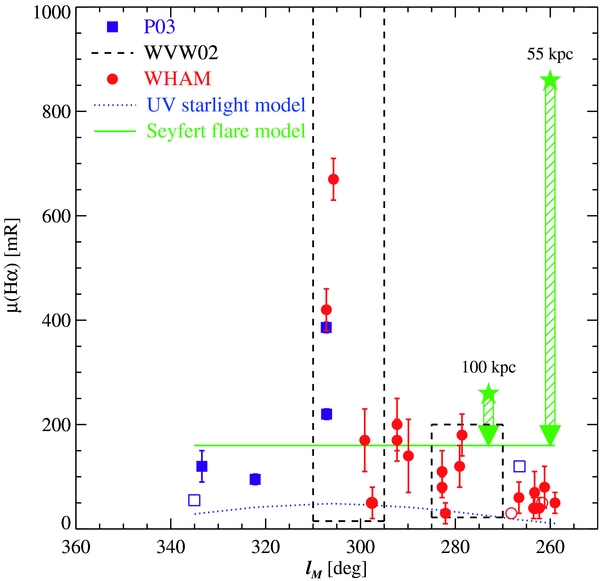
Figure 2. Observations and models of Hα emission along the Magellanic Stream. The dashed boxes indicate the range of detected values from Weiner et al. (2002); the purple points are from Putman et al. (2003); the red points are new observations from WHAM (Madsen 2012). The extreme Hα values occur close to the SGP at ℓM ≈ 303°. The dotted blue curve is the upper bound of allowed UV ionization from the Galaxy (disk+bulge+hot gas) from the model of Bland-Hawthorn & Maloney (1999). The green arrows illustrate the effect of a fading Seyfert flare for Stream distances of 55 kpc (long arrow) and 100 kpc (short arrow). The horizontal green line indicates a characteristic Hα surface brightness (160 mR).
Download figure:
Standard image High-resolution imageStream ionization. We adopt physically motivated units that relate the ionizing photon flux at a distant cloud to the resultant Hα emission. For this, we need to relate the plasma column emission rate to a photon surface brightness. In keeping with astronomical research on diffuse emission (e.g., WHAM survey; Reynolds et al. 1998), we use the Rayleigh unit introduced by aeronomers (q.v. Baker & Romick 1976) which is a unique measure of photon intensity; 1 milliRayleigh (mR) is equivalent to 103/4π photons cm−2 s−1 sr−1. The emission measure for a plasma with electron density ne is given by (e.g., Spitzer 1978)


which is an integral of H recombinations along the line of sight z multiplied by a filling factor fi. The suffix i indicates that we are referring to the volume over which the gas is ionized. For a plasma at 104K, cm−6 pc is equivalent to an Hα surface brightness of 330 mR. In cgs units, this is equivalent to 1.9 × 10⁻¹⁸ erg cm−2 s−1 arcsec−2 which would be a faint spectral feature in a 1 hr integration using a slit spectrograph on an 8 m telescope. However, for the Fabry–Perot "staring" technique employed in Figure 2, this is an easy detection if the diffuse emission uniformly fills the aperture. We refer to the Stream Hα emission as relatively bright because it is much brighter than expected for an optically thick cloud at a distance of 50 kpc or more from the Galactic center.

The characteristic Hα surface brightness observed along the Stream of μHα ≈ 160 mR (Figure 2) can be used to set a minimum required ionizing photon flux and luminosity for a Galactic center flare, assuming that the Stream emission has not begun to fade and that there is no absorption or extinction of the ionizing photon flux prior to reaching the Stream. For a slab ionized on one side, this is

The implied ionizing photon luminosities are then

for D = 55–100 kpc. Any model in which the Stream emission is produced by a nuclear outburst must explain the magnitude of this ionizing photon luminosity.
Expected emission via the Galactic stellar population. First we consider the expected emission due to the ionizing radiation from the Galactic stellar population and associated sources. The total flux at a frequency ν reaching an observer located at a distance D is obtained from integrating the specific intensity Iν over the surface of a disk, i.e.,

where n and N are the directions of the line of sight and the outward normal to the surface of the disk, respectively. At this stage, we consider only an isotropic illumination source rather than more complex forms of illumination with a strong polar angle dependence. In this instance, we use the more familiar scalar form of Equation (4) such that

where φ⋆ is the photoionizing flux from the stellar population, n · N =cos θ and h is Planck's constant. This is integrated over frequency from the Lyman limit (ν = 13.6 eV/h) to infinity to convert to units of photon flux (photons cm−2 s−1). The photon spectrum of the Galaxy is a complex time-averaged function of energy N⋆ (photon rate per unit energy) such that .

For a given ionizing luminosity, we can determine the expected Hα surface brightness at the distance of the Magellanic Stream. For an optically thick cloud ionized on one side, we relate the emission measure to the ionizing photon flux using cm−6 pc (Bland-Hawthorn & Maloney 1999). The total ionizing luminosity of the Galaxy is now well established within a small factor (Bland-Hawthorn & Maloney 1999; Weiner et al. 2002; Putman et al. 2003). For a total disk star formation rate of 1.1 ± 0.4 M☉ yr−1 (Robitaille & Whitney 2010), the hot young stars produce an integrated photon flux over the disk of 2.6 × 1053 photons s−1 with very few photons beyond 50 eV.

The mean vertical opacity of the disk at the Lyman limit is τLL = 2.8 ± 0.4, equivalent to a vertical escape fraction of f⋆, esc ≈ 6% perpendicular to the disk (n · N =1). The Galactic UV contribution at the distance D of the Magellanic Stream is given by

corresponding to φi ≃ 5.1 × 10⁴ photons s−1. The correction factor ζ ≈ 2 is included to accommodate weakly constrained ionizing contributions from the old stellar population, hot gas (disk+halo) and the Magellanic Clouds (Slavin et al. 2000; Bland-Hawthorn & Maloney 2002; Barger et al. 2013). We arrive at the blue curve presented in Figure 2 which fails to explain the observed Hα emission by at least a factor of 5.
If the Stream is more distant at 100 kpc, preferred by some recent models (Besla et al. 2012), the predicted emission measure due to the Galaxy approaches the upper limit (∼8 mR at 2σ) obtained by Weymann et al. (2001) for the cosmic UV intensity at the present epoch. The discrepancy with the observed Hα brightness is now a factor of 20!
Nuclear spectrum. We now consider the Stream emission due to ionizing radiation powered by the supermassive black hole at the Galactic center. Motivated by detailed spectral observations of AGN, we adopt a two-component accretion-disk model for the photon spectrum of the central source. We define the specific photon luminosity for the two-component model by

where if E > E1 and otherwise. The first term on the right-hand side of Equation (7) represents the cool, optically thin Shakura–Sunyaev spectrum thought to produce the enhanced UV ("big blue bump") emission observed in Seyfert galaxies and quasars (Antonucci 1993). The second term represents the X-ray and gamma-ray emission observed from the source. We choose E1 = 30 eV for the cool outer blackbody spectrum, α = 1.9 for the photon spectral index of the X-γ component (i.e., 0.9 for the energy spectral index), and adopt E2 = 100 keV (Dermer et al. 1997).
![$\mathcal{H}[E-E_1] = 1$](https://content.cld.iop.org/journals/0004-637X/778/1/58/revision1/apj485418ieqn6.gif)
![$\mathcal{H}[E-E_1] = 0$](https://content.cld.iop.org/journals/0004-637X/778/1/58/revision1/apj485418ieqn7.gif)
By integrating Equation (7) weighted by energy, we derive the relative normalization constants k1 and k2 (see Appendix C). The ionizing spectrum of NGC 1068 is strongly constrained by 2–200 μm Infrared Space Observatory (ISO)-Short Wavelength Spectrometer (SWS) observations (Alexander et al. 2000; Lutz et al. 2000). This barred spiral galaxy has the most extensive literature of any Seyfert and serves as a surrogate for the AGN activity at the Galactic center. We have used the unattenuated spectrum to normalize our composite model. We find that η ≈ 9 (log k1/k2 = 8.8663) provides a reasonable match to NGC 1068. Our assumed ionizing spectrum of the Galaxy's AGN presented in Figure 3 has the same functional form.

Figure 3. Energy spectrum of the Galactic center accretion disk (see Appendix C) is assumed to comprise a "big blue bump" and an X-ray +γ-ray power law component. The lower curve is the photon spectrum E · N•(E). The upper curve is the energy-weighted photon spectrum E2 · N•(E) which serves to illustrate that there is an order of magnitude more energy in the big blue bump (η = 9) than the hard energy tail. The data points are taken from the nuclear ionizing spectrum derived from the ISO-SWS (2–200μm) satellite data for NGC 1068.
Download figure:
Standard image High-resolution imageThe ionizing flux φ• follows from Equation (7) such that where IH = 13.598 eV. The spectrum is dominated by the soft component such that estimates of the AGN-induced Hα emission (below) are not obfuscated by the longer mean free paths of the harder photons. Thus properties derived from the stellar (φ⋆) and AGN (φ•) photon fluxes can be compared directly; the photons propagate roughly the same depth into an H i cloud.

Expected emission from an active nucleus. We now relate the accretion disk luminosity L• to the properties of the supermassive black hole. An accreting black hole converts rest-mass energy with a conservative efficiency  = 5% into radiation with a luminosity ()


for which is the mass accretion rate. The accretion disk luminosity can limit the accretion rate through radiation pressure. The so-called Eddington limit is given by


where M• is the black-hole mass and σT is the Thomson cross-section for electron scattering.
Radiation pressure from the accretion disk at the Galactic center limits the maximum accretion rate to M☉ yr−1. Some Seyferts, including NGC 1068 (Begelman & Bland-Hawthorn 1997), radiate at close to the limit, but active galactic nuclei appear to spend most of their lives operating at a fraction fE of the Eddington limit with rare bursts arising from accretion events (Hopkins & Hernquist 2006). For clouds at a distance of 55–100 kpc along the SGP, we now show that only a fraction of the maximum accretion rate is needed to account for the Hα emission along the Magellanic Stream. The orbital period of the Stream is of the order of a Hubble time so we can consider the Stream to be a stationary target relative to ionization timescales.

The dust levels are very low in the Stream (Fox et al. 2013); internal and line-of-sight extinctions are negligible. It follows from Equation (10) that the ionizing photon luminosity of the Seyfert nucleus is given by

For the photon spectrum in Equation (7), we find that 20% of the energy falls below the Lyman limit and therefore does not photoionize hydrogen. If the absorbing cloud is optically thick, the ionizing flux can be related directly to an Hα surface brightness. The ionizing flux is given by

We have included a term for the UV escape fraction from the AGN accretion disk f•, esc (n · N = 1). This is likely to be of the order of unity to explain the integrated energy in observed ionization cones (Sokolowski et al. 1991; Mulchaey et al. 1996). Some energy is lost due to Thomson scattering but this is known to be only a few percent in the best constrained sources (e.g., NGC 1068; Krolik & Begelman 1986). In principle, the high value of f•, esc can increase f⋆, esc but the stellar bulge is not expected to make more than a 10%–20% contribution to the total stellar budget (Bland-Hawthorn & Maloney 2002); a possible contribution is accommodated by the factor ζ (Equation (6)).
The expected surface brightness for clouds that lie within a putative "ionization cone" from the Galactic center is given by

Strictly speaking, this provides us with an upper limit or "peak brightness." In Section 3, we show that proper consideration must be given to the physical state of the gas and the time since the event occurred. The recombination emission will fade once the burst duration has passed and the gas begins to recombine and cool. For completeness, we have included a beaming factor b to accommodate more exotic models that allow for mild beaming of the UV radiation (e.g., Acosta-Pulido et al. 1990). The solid angle subtended by a half-opening angle of θ1/2 is . So the beam factor expresses how much of the isotropic radiation is channeled into a cone rather than 2π sr. For example, θ1/2 = 22 5 is a beam factor b = 13; θ1/2 = 30° is a beam factor b = 7.5; θ1/2 = 90° is a beam factor b = 1 (isotropic emission) adopted for the remainder of the paper. The emission within an ionization cone can be isotropic if the restriction is caused by an external screen, e.g., a dusty torus on scales much larger than the accretion disk.


3. PAST AGN ACTIVITY
3.1. Timescales
Consider the situation in which we observe the ionization of the Stream due to a nuclear source. A burst of intense UV at a time To in the past, lasting for a period TB, must propagate for a time TC ∼ 0.18 (D/55 kpc) Myr to reach the Stream. For example, in the Seyfert jet model of Guo & Mathews (2012), To ≈ 1–3 Myr and TB ≈ 0.1–0.5 Myr. The ionization front then moves through the cool gas until the UV is used up. This occurs in a time TI ∼ 1/(σHφ•) where σH is the H ionization cross section. This follows from the fact that the speed of the ionization front into the neutral gas is q = φ•/nH where q is the ionization parameter6 for a neutral H density nH. For the Hα emission levels associated with the Magellanic Stream, TI ∼ 4 × 10³/(φ•/106) yr; for simplicity, the extra factors from Equation (12) are not carried over. The time for the gas to reach ionization equilibrium will be of the order of TI, and is very short compared to both TC and the likely values of To. The Hα emission is then proportional to αBneNe, where ne is the electron density, Ne is the column density of ionized gas, and αB is the Case B recombination coefficient.
Since the level of activity in the Galactic Center today is far too low to produce the observed Hα emission, the Stream emission in this picture is almost certainly fading from an earlier peak. The time Td required for the emission to decrease from its peak value to the observed brightness depends on both the time evolution of the burst luminosity and the gas density in the Stream.7 Since we observe the Stream as it was TC years ago, the look-back time to the initial event is To = Td + 2TC (assuming the burst time TB is much less than To). We now revisit these approximations with detailed calculations of the ionization state of the gas.
3.2. UV Photoionization
We use the recently completed MAPPINGS IV code (Dopita et al. 2013) to study both isochoric and isobaric cooling at the surface of the Magellanic Stream. The source of the impinging radiation field is the accretion disk model presented in Figure 3. The MAPPINGS IV models were run by turning on the source of ionization, waiting for the gas to reach ionization/thermal equilibrium, and then turning off the ionizing photon flux. In Figures 4 and 5, we present our modeled trends in gas temperature (Te), ionization fraction (χ) and emission measure () for time-dependent ionization of the Magellanic stream. Important properties of the medium—ionized column depths, emission measures, cooling times, etc.—are included in Table 1. The sound crossing times of the warm ionized layers are too long (≳10 Myr) in the low density regime relevant to our study for isobaric conditions to prevail. Both a near (D = 55 kpc) and a far (D = 100 kpc) distance is considered.


Figure 4. MAPPINGS IV time-dependent isochoric calculations of the change in Hα surface brightness after a Seyfert flare has occurred at the Galactic center. Left: D = 55 kpc, fE = 0.1; right: D = 100 kpc, fE = 0.1. From left to right, the pre-ionized gas densities are 1.0, 0.3, 0.1, 0.03, and 0.01 cm−3. The clouds have 0.1 Z☉ metallicity and are irradiated by an AGN accretion disk (see text). The mean surface brightness of the Stream near the SGP (160 mR) is shown as a horizontal dashed line. Physical properties of the models are to be found in Table 1.
Download figure:
Standard image High-resolution image
Figure 5. MAPPINGS IV time-dependent calculations of how the ionized surface of a dense gas clouds cools with time: left: electron temperature Te; right: ionization fraction χ. We show the isochoric (constant density) models where the densities in cm−3 are indicated; isobaric models cool twice as fast at late times. The H i clouds have 0.1 Z☉ metallicity and are irradiated at D = 55 kpc by an AGN accretion disk (fE = 0.1) at the Galactic center (Figure 3).
Download figure:
Standard image High-resolution imageTable 1. MAPPINGS IV Time-dependent Ionization Calculationsa
| nH | dm | μHα | μHα | Td | To |
|---|---|---|---|---|---|
| (cm−3) | (pc) | (cgs) | (mR) | (yr) | (yr) |
| (a) 55 kpc | |||||
| 1.0 | 9 | 4.8e-18 | 844 | 1.3e5 | 4.9e5 |
| 0.3 | 63 | 4.8e-18 | 848 | 4.3e5 | 7.9e5 |
| 0.1 | 404 | 4.8e-18 | 849 | 1.4e6 | 1.8e6 |
| 0.08 | 1423 | 4.8e-18 | 852 | 1.8e6 | 2.9e6 |
| 0.03 | 3461 | 4.9e-18 | 858 | 4.7e6 | 5.1e6 |
| (b) 100 kpc | |||||
| 1.0 | 4 | 1.4e-18 | 251 | 3.0e4 | 7.5e5 |
| 0.3 | 31 | 1.5e-18 | 258 | 1.0e5 | 8.2e5 |
| 0.1 | 178 | 1.5e-18 | 258 | 3.2e5 | 1.0e6 |
| 0.03 | 1345 | 1.5e-18 | 257 | 1.2e6 | 1.9e6 |
| 0.01 | 9230 | 1.5e-18 | 259 | 4.2e6 | 4.9e6 |
Notes. aSeyfert flare model (fE = 0.1) using two distances (D = 55, 100 kpc) for the Magellanic Stream. The columns are: (1) hydrogen gas density; (2) depth of ionized layer integrated to 90% neutral; (3) Hα surface brightness in erg cm−2 s−1 arcsec−2; (4) Hα surface brightness in mR; (5) time for the ionized gas to cool down to mR; (6) look-back time To = TR + twice the light propagation time (TC). Bold rows are consistent with the known gas properties of the Stream.

Download table as: ASCIITypeset image
The gas phase abundances are the solar values scaled to [Fe/H] = −1 now well established from Hubble Space Telescope COS measurements (Fox et al. 2013; Richter et al. 2013). The upper limits for [O i] 630 nm from the WHAM survey indicate that the ionization fraction in the brightest Hα-emitting clouds exceeds χ = 50% (G. Madsen et al. 2013, in preparation). For a spherical cloud, its mass is approximately where the subscript n denotes that the filling factor refers to the neutral cloud prior to external ionization. For a fixed cloud mass (or equivalently, cloud column density Nc), the filling factor is inversely related to the H i gas density. Any value other than unity leads to higher gas densities and shorter recombination times. While the cloud geometry and the volume filling factor are uncertain (Fox et al. 2010), self-consistent ionization parameters q are obtained at all times and lie within the range log q = 5.6–7.6 (log u ≈ −5 to −3).

In Figure 5, the initial photoionizing flash rapidly heats the gas to a peak temperature before the gas begins recombining at a rate that is inversely proportional to nH as expected (Section 2). We observe that the recombination rate is faster than the cooling rate during this period. The initial flash produces high ionization states (e.g., He ii, [O iii] emission lines), but these fade rapidly. In Figure 4, the increase in electron density leads to a maximum Hα brightness which then also fades. The Balmer decrement Hα/Hβ is everywhere in the range 3.0–3.1 until very late times when it begins to climb, except now the flare ionization signal has almost faded from view. While the decrement is sensitive to dust extinction, the low metallicity of the Stream has negligible impact on this diagnostic (see Section 5). At late times, the Hα surface brightness in all cases scales as t−2; see Appendix A.
In Table 1, we show key properties of the models as a function of the pre-ionization gas densities. The realistic cases are shown as emboldened values where we have ignored small factor uncertainties; the remaining models exceed the properties (either local or column density) of the Stream clouds. Column 5 shows the times Td for the emission to drop to the canonical surface brightness of 160 mR (see Figure 2). The look-back times are shown in Column 6; note that the light propagation time (2TC) dominates the high density extremes. These timescales are in line with published models of the Fermi bubbles (Section 1). The lower ionizing flux at the 100 kpc distance (since the peak luminosity in the models is fixed) leads to shorter look-back times because the gas requires less time to reach 160 mR.
Distance vs. flare luminosity. It is clear from Figure 4 that lower ionizing fluxes or larger Stream distances lead to shorter inferred timescales for the Seyfert flare event. To within a small factor, the ionization model (D, fE) = (55 kpc, 0.1) is equivalent to the (100 kpc, 0.3) model once all timescales are considered. Conversely, the ionization model (D, fE) = (100 kpc, 0.1) is equivalent to the (55 kpc, 0.03) model. In Appendix A, we present a simplified model for the evolution of the ionization fraction and Hα surface brightness from the Stream which is in good agreement with the MAPPINGS IV models shown in Figure 4, which we use to discuss in more detail the constraints that can be placed on the flare energetics and evolution in Section 5.1.
Variations in Hα brightness. An attractive aspect of the Seyfert flare model is the ability to accommodate the brightest Hα measurements and the scatter about the elevated mean surface brightness (160 mR) compared to the expective Galactic ionization level. An interesting question is whether the scatter reflects variations in gas density (geometry) or photon arrival time (finite TB). In Figure 6, we show the relation between μHα and nH at a fixed time over a range of times from 0.5 Myr to 5 Myr. For an impulsive burst, it is possible to accommodate all of the detections at a fixed time, certainly within the first few Myr of the Seyfert event. However, the very short ionization timescale TI (Section 3.1) means that we are unlikely to see temporal variations of the source: the Stream emission is unaffected by any variations in incident ionizing flux that occurred longer than ∼TI ago. Source luminosity variations on longer timescales will be modulated by a transfer function that depends on the gas density (see Appendix A); any observable fluctuations in Hα are likely the result of variations in density and hence recombination timescale. The most relevant epoch in interpreting the Stream emission is the end of the flare.

Figure 6. MAPPINGS IV time-dependent isochoric calculations of the change in Hα surface brightness after a Seyfert flare has occurred at the Galactic center (D = 55 kpc, fE = 0.1; Z = 0.1 Z☉). The canonical Stream brightness (160 mR) is shown as a horizontal dashed line. The tracks plotted every 0.5 Myr show the relation between Hα and gas density at a fixed recombination time TR. The associated look-back times (offset by the light crossing time) are shown in Table 1. The dark vertical band shows the range in nH consistent with the known cloud properties; the lighter band is marginally consistent.
Download figure:
Standard image High-resolution image4. FUTURE TESTS OF THE MODEL
In Seyferts with moderately low mass black holes, the jet/wind/cone axis can be strongly misaligned with the spin axis of the galaxy (Cecil 1988; Mulchaey et al. 1996) but there are many counter examples (Duric et al. 1983; Wehrle & Morris 1987, 1988; Keel et al. 2006). The Fermi bubbles and the X-ray bipolar structure are roughly aligned with the SGP. These features fill most of the conic volume in our model within 10 kpc, and presumably the outflow has swept any halo gas aside. We assume that the ionization cone in the Seyfert flare model is also aligned with the SGP (ℓM ≈ 303°). Thus, to account for the brightest clouds in the Stream (Figure 2), the half-opening angle θ1/2 of the cone is at least 25° to accommodate enhanced emission at the same angle from the SGP (ℓM ≈ 278°).
Any gas clouds caught within the cones at smaller distances will be roasted by the Seyfert nucleus. However, almost all the known high velocity clouds reside close to the Galactic Plane (b < 30°; Putman et al. 2012). There are few known HVCs close to the SGP although evidence for ionized HVCs has been presented (Lehner & Howk 2010). In our model, most of the HVCs will be fully ionized within the ionization cone. Interestingly, there is one sight line close to ℓM = 308° where the Hα surface brightness is up to four times higher than our benchmark flare value of 160 mR (Figure 2). A possible explanation is that some of the Stream clouds are somewhat closer than the canonical distance of 55 kpc.
A competing model for the Hα emission uses a radiative hydrodynamic simulation to demonstrate the possibility of a slow shock cascade acting along the Stream (Bland-Hawthorn et al. 2007). Arguably, this is the only serious attempt to date to explain the Stream Hα emission. However, this model does not work well if the Stream at the SGP is at the larger distance of D ≈ 100 kpc. Given that one end (front) of the Stream is tied to the LMC–SMC system, this would require the far trailing end (back) of the Stream to subtend a large angle to the halo, being more radial than tangential to the halo. This has two problems: (1) the Hα emission would be almost entirely confined to the front of the Stream; (2) the back of the Stream would be undetectable.
For the near distance of D = 55 kpc, for most optical diagnostics, the slow shock cascade may be difficult to disentangle or distinguish from our model of AGN photoionization. The diluteness of the predicted AGN field, with ionization parameters in the range log q = 5.6–7.6 (log u ≈ −5 to −3), tends to produce shock-like emission line diagnostics. The high energy part of the big blue bump (50–100 eV) can excite He ii and [O iii], with enhanced ratios to Hβ of about 0.3 and 1, respectively, but these occur at the peak of the flash and fade rapidly, and only for the near-field Stream (Figure 4(a)). The high energy tail in Equation (7) can excite a few atoms with high ionization cross sections but the radiation field in X-rays is very dilute, and the metal fraction is low ([Fe/H] ≈−1; Fox et al. 2013).
We are presently re-running the shock cascade models at higher resolution and with the updated ionization diagnostics in MAPPINGS IV. This will be the focus of a later paper. The shock cascade has a slightly elevated density-weighted temperature (Te ≳ 12, 000 K) compared to the time-averaged Seyfert flare model (Te ≈ 10, 000 K), but both models produce comparable emission in the optical diagnostic [S ii], [N ii], and [O i] emission lines.
A promising diagnostic is the Balmer decrement Hα/Hβ which is typically enhanced in slow shock models (Bland-Hawthorn et al. 2007). The dust content in the Magellanic Stream has negligible impact on this line ratio. Diffuse optical detection surveys to date have largely focused on the 500–700 nm window in part because Hβ is harder to detect along most of the Stream (Reynolds et al. 1998). In our Seyfert flare models, the Balmer decrement at the distance of the Stream is in the range 3.0–3.1 for detectable emission, rising slowly at late times when the recombination emission has largely faded. In the shock cascade model, the Balmer decrement exceeds 3.1 and can reach values that are 50% higher.
5. NEW INSIGHTS ON AGN ACTIVITY
5.1. Accretion Disk
Sgr A⋆ provides us with a front-row seat on the daily life of a supermassive black hole.8 Nuclear activity today at the Galactic center is remarkably quiescent given the rich supply of unstable gas within the circumnuclear disk (Requena-Torres et al. 2012). This observation has driven the rapid development of accretion disk models over the past 20 yr: a comprehensive review is given by Genzel et al. (2010). It is now believed that Sgr A⋆ is a radiatively inefficient accretion flow (RIAF) fueled by poor angular momentum transport at all radii in part due to strong outflows and convection in the innermost accretion zone (Blandford & Begelman 1999; Hawley & Balbus 2002; cf. Jolley & Kuncic 2008).
The observed material within a few parsecs of Sgr A⋆ can readily account for the 0.02–0.2 M☉ yr−1 accretion rate required in our model. Stellar accretion events are expected once every 40,000 years on average (Freitag et al. 2006). There are indications of infalling gas clouds over the past 10 Myr. One such cloud impact possibly triggered the formation of a kinematically distinct ∼104 M☉ cluster within ∼0.1 pc of Sgr A*, traced by ∼80 massive young stars with ages in the range 2.5–8 Myr (Paumard et al. 2006; Lu et al. 2013). Wardle & Yusef-Zadeh (2008) draw attention to the "+50 km s−1 cloud" known to have passed through the Galactic Center within the last 1 Myr. These events bracket our inferred epoch for the Seyfert flare which may have been causally linked to one of these or a related event.
We do not know what the peak luminosity of the burst was, or the timescale on which it decayed. Such information would shed light on the nature of the accretion event, whether an individual star (TB ∼ 102–3 yr) or an infalling cloud on much longer timescales. However, we can use the simplified model for the Stream emission developed in Appendix A, which is in good agreement with the detailed MAPPINGS IV results for the time-dependent Hα surface brightness, to place constraints on these quantities.
As in Appendix A, define ρ to be the ratio of the observed μHα to its peak value. This is also equal to the ratio of the minimum required ionizing flux (Equation (2)) or ionizing luminosity (Equation (3)), to their peak values, as well as the minimum required value of the Eddington fraction fE, min to its peak during the burst. Using Equations (2) and (12) for the ionizing flux from the AGN (with f•, esc set to 1), we can write this minimum Eddington fraction as

In the limit where the e-folding time for decay of the burst τs is much shorter than the recombination timescale τrec, we have the analytic result

where τo is the dimensionless age of the burst as measured in recombination times. (This is simply another form of Equation (A23)). Using Equation (A9) for τrec and Equation (14) for fE, min, we have calculated the required peak value of fE as a function of gas density nH and burst age To, for both D = 55 kpc and 100 kpc. Assuming that the present-day Eddington fraction of Sgr A⋆ is ∼10−8 (Genzel et al. 2010), we can also calculate the required value of the e-folding time τs: the inferred value of peak fE at a given To determines the number of e-folding times that have passed in the age of the burst.
The results are shown in Figure 7. The grey upper right portion of the diagrams is where fE, peak exceeds 1; this occurs sooner at higher nH (more recombination times) and larger To (more e-folding times τs). This condition is violated more readily for D = 100 kpc, since a greater φi is needed to produce the same Hα surface brightness; this also means the minimum allowed value of fE is ∼3.3 times larger. However, a broad range of reasonable fE is allowed for burst ages greater than ∼1 Myr in both cases; a larger Stream distance favors lower nH (to increase τrec) and larger fE, peak.

Figure 7. Constraints on the Sgr A* burst peak Eddington fraction fE, peak (blue contours) and burst decay e-folding time τs (magenta contours) as a function of Stream gas density nH and burst age To, for the case of very rapid burst decline. The gray region requires fE > 1. Left: D = 55 kpc. Right: D = 100 kpc.
Download figure:
Standard image High-resolution imageAlthough we have assumed that τs → 0 in Figure 7, the results are not very sensitive to this assumption: in Appendix A, we show that τrec/τs is likely to be a factor of order a few; for these values, there are modest shifts of the curves from the instantaneous decline case (see Figure 10 in Appendix A).
In our interpretation, Sgr A⋆ was far more active in the past. Rapid and stochastic variations in AGN activity are to be expected (Novak et al. 2011, 2012). Depending on the Stream distance, for plausible nH and To the required Eddington fraction fE is of order 0.03–0.3 which is a factor of 107–8 times higher than the quiescent state today.9 The most extreme event witnessed in models by Novak et al. (2011, their Figure 6) is a transition from fE ∼ 10−3 to fE ∼ 3 × 10⁻⁸ in a few Myr (45 dB). This happens when there is a lot of material in the accretion disk around the black hole. The AGN heats up the interstellar medium and terminates additional infall, and then the mass drains out of the disk with an e-folding time of about 0.1 Myr. The timescale of the drop is roughly the characteristic time to clear the accretion disk (G. Novak 2013, private communication).
However, our new result demands 70–80 dB suppression within a time frame of only ∼1–5 Myr. Such a rapid variation requires an extremely efficient and well confined "drip line" to prevent the fresh gas from being sheared by the accretion disk which would wash out extreme fluctuations in UV luminosity (S. Balbus 2013, private communication). Magnetic fields—required to mediate angular momentum transport—are expected to thread through a RIAF disk and these are almost certainly needed to achieve the severe confinement and rapid fuelling.
In time, we may learn about the detailed structure of the evolving accretion disk before, during and after a major outburst (Ho 2008). If the Seyfert flare model is ultimately confirmed to be the correct explanation for the Stream's partial ionization, it provides us with a very interesting and spatially resolved probe of the escaping radiation. We refrain from considering more sophisticated accretion disk/jet models, with their attendant beaming, until more progress is made in establishing the true source of the ionizing radiation and the Stream's trajectory. A stronger case must be made for preferring this model over another (i.e., the shock cascade), but we note that the green horizontal line in Figure 2 is not a good fit to most of the data points. An inverted low amplitude parabola centered on the SGP does better. This can be understood in terms of an accretion disk radiation field with a polar angle component; such models have been presented (e.g., Madau 1988; Sim et al. 2010). However, the trend to lower Magellanic longitude can conceivably be explained if the Stream subtends a large angle to the Galactic halo.
5.2. UV Line-driven Wind
It is evident that the explosive nuclear activity that created the extended X-ray, microwave, and gamma-ray radiation gave rise to a large-scale outflow from the Galactic center. Both starburst and AGN activity are likely to be operating from the central regions. While their time-averaged energetic outputs may be similar, they operate with very different duty cycles and temporal behavior (Alexander & Hickox 2012). The Fermi observations have been discussed extensively in the context of accretion disk activity associated with the well established supermassive black hole (Su et al. 2010; Guo & Mathews 2012) although alternative starburst models have been presented (Carretti et al. 2013). Starbursts drive large-scale winds very effectively and may assist with the observed bipolar activity. As already mentioned (Section 1; see also Appendix B), starburst activity cannot account for the Stream Hα emission.
Is it possible to associate the powerful radiative phase with the wind phase? Regrettably, there are few published accretion disk models that provide both the ionizing luminosity and mechanical luminosity of the central source. For our discussion, we use the well prescribed models of Proga & Kallman (2004, hereafter P-K) that build on their earlier work (Proga et al. 2000).
In the P-K wind models, the relatively high radiation UV flux and opacity (mainly due to line transitions) supply a strong radiative force that is able to lift gas over the photosphere. This gas provides significant column density to block the X-rays otherwise the wind becomes overionized and the flow switches off. The line-driven wind is launched from the part of the disk where most of the UV is emitted. In effect, the inner disk wind shields the outer wind. The high value of η in Equation (7) is consistent with our assumption that the UV radiation dominates over X-rays and powers the large-scale wind (Proga et al. 2000).
The P-K wind reaches velocities roughly twice the escape velocity from the launching region. So this gives velocities of about 10,000 km s−1 for a system with M• = 108 M☉ although maybe somewhat less for the supermassive black hole associated with the Galactic center. With this velocity it will take only 0.1 Myr to reach a distance of 1 kpc, and 1 Myr to reach 10 kpc. The disk wind mass loss rate is roughly 10% or so of the disk accretion rate and therefore does not cause a significant reduction of the accretion rate. The wind is unlikely to ionize cold gas at the distance of the Stream.
Using the Proga models, Sim et al. (2010) computed spectral energy distributions as a function of viewing angle as seen from the accretion disk. They compute the photionization and excitation structure of the wind and track multiple scattering of the photons. The polar radiation field depends on photon energy and the escaping radiation is confined to a cone. The X-ray and the UV radiation come from different directions; the former propagate parallel to the UV photosphere whereas the latter is normal to it. Therefore, the column density for the X-rays is much higher than for the UV as expected, although some leakage is observed.
We observe that something like this may be happening in detailed observations of nearby active galaxies. In an integral field study of 10 galactic winds, Sharp & Bland-Hawthorn (2010) compared five starbursts and five AGNs. The AGN winds show clear evidence for non-thermal ionization from the central source across the wind filaments to the radial limits of the data. However, AGN ionization cones are not always associated with winds. For example, the most famous of the Seyfert ionization cones is NGC 5252 (Tadhunter & Tsvetanov 1989) which is not associated with an energetic outflow. In the context of the P-K model, we associate these cones with AGNs where strong X-rays escape from the nucleus which serve to suppress the line-driven wind. This distinction may become less clear cut if more powerful line-driven winds (presumably from more massive black holes) are able to drive shocks in the gas along the ionization cone. Thus ionization cones may be detectable in X-rays even while the central source irradiates the cone exclusively with UV. Shocked gas tends to radiate at a higher temperature compared to photoionized gas, and this may allow these cases to be separated.
Line-driven winds struggle with black hole masses as low as that associated with Sgr A⋆ unless the accretion rate is close to the Eddington limit. If the Stream ionization is due to a burst of radiation from a P-K disk, then fE ∼ 1 is an order of magnitude more than is need to account for the observed Hα emission for the canonical Stream distance (55 kpc), although it would aid ionization of the Stream at the larger distance. In principle, f•, esc could be lower than our assumed value of 100%, but the high limit is consistent with what we know about ionization cones (e.g., Mulchaey et al. 1996) and is a consequence of the P-K wind model where the wind has cleared a channel for the UV emission (Proga & Kallman 2004; Sim et al. 2010).
6. CONCLUSIONS
We have shown how the Magellanic Stream is lit up in optical emission lines at a level that cannot be explained by disk or halo sources. A possible explanation is a shock cascade caused by the break-up of clouds and internal collisions along the Stream (Bland-Hawthorn et al. 2007) but this becomes untenable if the Stream is much further than the canonical distance of 55 kpc.
We have introduced time-dependent ionization calculations with MAPPINGS IV for the first time in order to present a promising Seyfert flare model that adequately explains the observed photoionization levels along the Magellanic Stream. The model works at both the near and far Stream distances, and can be tested in future observations. A "slow shock cascade" is expected to produce a steeper Balmer decrement (Hα/Hβ > 3.1) than the flare model. Since the Magellanic Stream has a very low dust fraction ([Fe/H] ≈−1), this is likely to be the most accessible discriminant between the models. Other useful diagnostics (He ii/Hβ, O iii/Hβ) reach peak values shortly after the Seyfert flash but fade rapidly.
We cannot yet identify the specific event which triggered the burst of Seyfert activity although the stellar record tells us the past 10 Myr have been very active (Ponti et al. 2013). The time lag between an accretion event and the onset of starburst or AGN activity (or how these operate together) is a major unsolved problem in astrophysics. The inner tens of parsecs provide many possible cloud candidates, assuming it was not largely consumed, many on highly elliptic orbits. If our model is correct, it provides many new challenges for the burgeoning field of Galactic Centre research. Regardless of the origin of the emission, the Stream provides an important constraint on past AGN activity and on models that attempt to explain the Fermi gamma-ray bubbles.
This work came about during the 2013 April "Fermi Bubbles" workshop held at KIPAC Stanford organized by Dmitry Malyshev and Anna Frankowiac. We acknowledge insightful conversations with Steve Balbus, Bill Mathews, Daniel Proga, Greg Novak, Bruce Draine, and Kyler Kuehn. J.B.H. is indebted to James Binney for early comments on the manuscript. We are particularly grateful to Roger Blandford and the participants of the Kavli workshop without whom this paper may not have been realized. We thank the referee for suggestions that led to more detailed discussions in Appendices A and B.
APPENDIX A: A SIMPLE MODEL FOR TIME-DEPENDENT EVOLUTION OF THE IONIZATION FRACTION AND Hα SURFACE BRIGHTNESS
Consider the following simple model for the Stream clouds: a uniform density gas of pure hydrogen, with a photon flux φi normally incident upon it. If the gas has been exposed to the ionizing photons for long enough to reach ionization equilibrium, then all of the photons will be absorbed in a length L given by

where α is the recombination coefficient. This is just the condition that the column recombination rate equals the incident flux. Thus,

To simplify even further, assume that for depth d < L into the Stream gas, the gas is completely ionized, while for d > L, it is neutral. Hence, all the emission measure comes from d < L, and we will also ignore any effects of absorption on φi, so the region with d < L can be treated as uniform.
Now suppose that the ionization rate decreases from the initial value for which the equilibrium was established. Without loss of generality, we can assume an exponential decline for φi, with a characteristic timescale for the ionizing source τs (Sharp & Bland-Hawthorn 2010). The time-dependent equation for the electron fraction xe = ne/nH is

where ζ is the ionization rate per atom.
Consider first the case where τs → 0, so that φi declines instantaneously to zero. Then the second and third terms in Equation (A3) vanish, and we just have

This is easily solved with the substitution , and with the initial condition xe = 1 at t = 0 we get


Defining the recombination timescale

this is simply

To evaluate Equation (A7) for the conditions in the Stream, we use αB = 2.6 × 10⁻¹³ cm3 s−1 for the recombination coefficient (appropriate for hydrogen at 104 K), and use the fiducial values φi = 106φ6 photons s−1, nH = 0.1n−1 cm−3. Then


and the emission measure

so the gas density enters explicitly only through the recombination time. The resulting Hα emission will be

or, with Equation (A7)

In the left-hand panel of Figure 8, we plot the prediction of Equation (A12) for the Hα surface brightness as a function of time for φ6 = 2, as used in Equations (10) and (11) for D = 55 kpc. Comparison with the left-hand panel of Figure 4 shows that this simple model agrees well with the detailed MAPPINGS IV results, except for the highest densities. The discrepancy is largely because Equation (A12) predicts that xe depends only on t/τrec, and hence xe remains close to unity (and thus μHα at its peak value) only if t/τrec is small, but that is not true for the highest densities at the earliest times for the range of times that are plotted. However, it clearly does a good job of reproducing the late-time behavior (μHα∝(t/τrec)−2), to which all the models in Figure 4 asymptote.

Figure 8. Left: the Hα surface brightness as a function of time predicted by Equation (A12), for φ6 = 2. From left to right, the curves are for gas density nH = 1, 0.3, 0.1, 0.03, and 0.01 cm−3. Right: the evolution of the Hα surface brightness (scaled to the peak brightness) with dimensionless time τ obtained by solving Equation (A16) for several values of the ratio β of recombination time to ionizing photon flux decay time. Curves are labeled with β; all models assume a ratio of recombination to t = 0 ionization time γ = 240.
Download figure:
Standard image High-resolution imageEquation (A3) does not have an analytic solution when the time-dependence of φi is included. However, it is easily solved numerically and can be transformed into a more useful form with some trivial definitions. Define the dimensionless time τ by

τ is simply the time measured in units of the recombination time. In addition, define

where is the ionization time at t = 0, and


the ratio of recombination to ionizing photon luminosity e-folding times. Then Equation (A3) becomes

We can write the ionization rate per H atom as

where σ0 is the H ionization cross-section at threshold and Ci is a constant of order unity that depends on the shape of the spectrum. The ionization time then evaluates to


and we can write γ as (using Equation (A9) for τrec)

The resulting Hα surface brightness obtained from the solution of Equation (A16) for the ionization fraction, normalized to the peak value, is shown in the right-hands panel of Figure 8 for γ = 240 and values of β from 0.2 to ∞ (τs → 0, the case shown in the left-hand panel). However, an important point from this analysis can be derived simply from the form of Equation (A16). As just shown, γ must be large—this is inevitable from the assumption that the gas in the Hα-emitting region is highly ionized to begin with. Hence the ionization fraction (and thus the Hα surface brightness) will not begin to decrease substantially until

and thus until τ reaches the critical value

Physically, this is just a reflection of the requirement that the ionization time must be longer than the recombination time before the ionization fraction begins to drop. If β ≲ 1—the ionizing photon flux is decreasing on a timescale longer than the recombination timescale—the ionization fraction (and thus the Hα emission) will not begin to decline substantially until many recombination times have passed.
The numerical solutions of Equation (A16) show that the expression (A21) for the critical time is quite accurate: for γ = 240, it predicts τc ∼ 0.55, 5.5, 11, and 27 for β = 10, 1, 0.5, and 0.2, respectively. Since τc depends only logarithmically on φi and the gas density nH, the precise values of these quantities are unimportant—all that matters is that, generically, ln γ ∼ a few. Unless τs is much shorter than τrec (β ≫ 1), the decline of xe—and thus of μHα—is substantially delayed from the instantaneous φi turn-off case. (Note also that for β < 1, the decline is steeper once it begins. This is because the derivative of xe with respect to ln τ has its maximum at τc—physically, there is simply more time available between the steps of ln τ at these later times.)
This simple model can also be used to address another very important issue. We do not know a priori what the peak luminosity of the burst was, or the timescale on which it decayed. All we know is that the peak Hα surface brightness was at least equal to the present epoch value. Define

This is also equal to the ratio of minimum to peak ionizing photon luminosity Ni, min/Ni, peak and to the ratio of the minimum required Eddington fraction to the peak value, fE, min/fE, peak. Consider first the limit of τs → 0. From Equation (A7), we have

(cf. Equation (A12)). The time needed for the Hα surface brightness to decline to its observed value, in units of the recombination time, is simply

The value of τρ predicted by Equation (A24) agrees reasonably well with the models presented in Figure 4. For D = 55 kpc, ρ ≃ 0.2, and so τρ = 1.24. Using Equation (A9) for τrec, the values from Table 1 give τρ = 1.08–1.2, while for the D = 100 kpc model, ρ ≃ 0.64, so the predicted value of τρ = 0.25, while the derived values range from 0.25 to 0.35. The differences between the prediction and the calculated values result from the simplification of Equation (A9) in assuming a constant recombination coefficient that is independent of time and ignores the different temperature histories as shown in Figure 5.
For the case of non-instantaneous decline of the burst luminosity, we can easily solve for τρ numerically for different values of β. One difference from the results shown in the right-hand panel of Figure 8 is that we must define γ consistently with the choice of ρ; this can be seen by noting that Equation (A14) for γ can be written, using Equation (2) for φi, min and Equation (A9) for τrec, as

which we use to specify γ as a function of ρ.
The solutions for τρ are shown in Figure 9. The left panel assumes a Stream gas density fixed at nH = 0.1 cm−3, and shows the results for several different values of β (as in Figure 7). The offset between the curves with different β is a direct reflection of the delay in the decline of μHα seen in the right-hand panel of Figure 8. In the right-hand panel of Figure 9, β has been fixed at 3 (see below), and τρ is plotted against ρ for several different densities. From Equation (A25), for fixed ρ the value of γ increases with decreasing density nH, which is why the curves flatten out as nH declines to the lowest values. The spread is much smaller than in the variable-β curves shown in the left-hand panel, especially for small values of ρ; this is because τc depends only on ln γ whereas it depends linearly on 1/β, as discussed above (Equation (A21)). The steep decline as ρ → 1 seen in both panels of Figure 10 is imposed by the initial condition xe = 1 at ρ = 1. The convergence of all the models to the same steep rise as ρ → 0 results from the negligibility of the ionization term at late times (τ ≫ τc), so that they all approach the solution (A7) for the instantaneous-decline case.


Figure 9. Left: the dimensionless time τ required for the Hα surface brightness to decline to a fraction ρ of its peak value; ρ is also equal to the ratio of the minimum ionizing photon flux or luminosity to their respective peak values. Curves are labeled with β, the ratio of recombination time to ionizing photon flux decay time. A Stream gas density of nH = 0.1 cm−3 was assumed. Right: as in the left panel, except for β fixed at 3 and different values of the gas density (labeled).
Download figure:
Standard image High-resolution image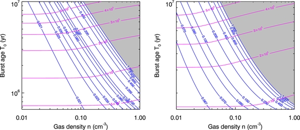
Figure 10. Required Eddington fraction as a function of burst age To and Stream gas density To. Left: for D = 55 kpc and β = 3. Right: for D = 100 kpc and β = 6. Compare with Figure 7.
Download figure:
Standard image High-resolution imageWe use these results in Section 5.1 to discuss the constraints on the peak luminosity and decay timescale of the Sgr A* flare. Here we note that β is likely to be at least a few. In terms of the Eddington fraction and the burst age To, we can evaluate Equation (A24) to get

for fE, peak = 1. This gives the largest possible value for τs. In Section 5.1, we infer a central flare that has faded by 80 dB, or approximately 18 e-folding times, since the burst peak. With Equation (A26), we then get that τs ≲ 4(2) × 105/nH for D = 55(100) kpc. This implies β ≳ 3 − 6 for the Stream distances: burst decay times longer than τs ∼ a few × 105 yr are unlikely, given the probable age of the Fermi bubbles. In Figure 10 we show the required value of Eddington fraction fE as a function of burst age To and gas density nH for these two cases. Comparison with Figure 7 in Section 5.1 shows that the differences from the case β → ∞ are modest.
We mention briefly one further important point. The gas recombination/cooling times can obscure any natural variations in the source ionizing luminosity. As discussed in the text, the Stream Hα emission must arise from a fading source, but the fading time of the Hα emission is limited by the gas recombination time, which imposes a transfer function on the luminosity variations. The source variation timescale τs could in principle be shorter, and the luminosity variations even more dramatic, than what we infer. In reality, the transfer function will be even more complex than what is implied by the simple model used here, since the real Stream gas has distributions of gas density and column density. In general, when comparing numerical models of AGN variability with the Stream emission (e.g., Novak et al. 2011), the modeled data stream must be temporally convolved with a function whose bandwidth will depend on the gas density.
APPENDIX B: THE IMPLAUSIBILITY OF A STARBURST ORIGIN OF THE FLARE
Equation (3) provides a minimum estimate for the ionizing photon luminosity needed to explain the Stream Hα emission of Ni ∼ a few × 1053 photons s−1—this assumes no fading of the emission and no significant absorption of the ionizing photon flux. What starburst parameters does this imply?
Maloney (1999) quotes a ratio of ionizing photon luminosity to star formation rate of

with substantial caveats on starburst age, upper and lower mass cutoffs, etc. This number agrees very well with the properties of the massive young star clusters formed in the Galactic center over the past several Myr: the Quintuplet, the Arches, and the Nuclear Cluster, which have total stellar masses ∼104 M☉, ages in the range 1–7 Myr, and Ni ∼ 1051 photons s−1 (Figer et al. 1999). Even for burst timescales as short as 1 Myr, the resulting star formation rates yr−1, giving ionizing photon luminosities per unit SFR in agreement with (B1). We can also use these observations to estimate the ionizing photon flux per unit mass of stars formed: this is


Powering the Stream emission at the minimal levels of Equation (3) thus requires a SFR of

and a total mass of stars formed of

The requirement of Equation (B3) exceeds by ∼ two orders of magnitude all estimates of the SFR in the Galactic center within the last 1–100 Myr (e.g., Pfuhl et al. 2011, their Figure 14, and many references therein; see also above). A similar problem arises with the mass of stars in the Galactic center as a function of age (Pfuhl et al. 2011). This number for the SFR is likely to be a substantial underestimate, since we have neglected extinction in the vicinity of the star-forming regions: for the three young Galactic center clusters discussed above, a large fraction of the emitted ionizing photons are absorbed locally.
In fact, the situation is even worse than this: any such nuclear starburst would have to have declined in luminosity by ∼2 orders of magnitude from the required peak luminosity to the present epoch, indicating that ∼5 or more e-folding times have elapsed. For plausible minimum starburst timescales (τs ∼ 2–3 Myr), this makes the burst epoch too early to match the age of the Fermi bubbles. Except for implausibly small Stream densities (n ∼ 0.01cm−3), this also indicates that β ≲ 1, and even though this will delay the decline of Hα surface brightness compared to the case where the flare shuts off in a time (see Appendix A), it also introduces a fine-tuning problem: unless we are catching the Stream emission at a time very close to τc as given by Equation (A21), the observed μHα will be substantially less than the peak value, indicating that the peak SFR and the mass of stars formed in the burst would need to be even larger than the estimates of Equations (B3) and (B4). Hence starburst models for the Stream Hα emission are simply not viable: the required star formation rates greatly exceed anything seen in the star formation history of the Galactic center.

APPENDIX C: SPECTRAL ENERGY DISTRIBUTION OF AN ACCRETION DISK
Our model for the accretion disk comprises a "cool" big blue bump and a "hot" power law component. We define the specific photon luminosity for the two-component spectrum by

where if E > E1 and otherwise. Then the total AGN luminosity is given by
![$\mathcal{H}[E-E_1] = 1$](https://content.cld.iop.org/journals/0004-637X/778/1/58/revision1/apj485418ieqn25.gif)
![$\mathcal{H}[E-E_1] = 0$](https://content.cld.iop.org/journals/0004-637X/778/1/58/revision1/apj485418ieqn26.gif)

where ≡ E/E1, μ ≡ E/E2, and w2 ≡ E1/E2.
Taking the hydrogen ionization potential, IH = 13.59844 eV, and w1 = IH/E1, the AGN ionizing luminosity is found by integrating from the Lyman limit to infinity,

where the limit for the second integral remains the same since w2 > w1.
The big blue bump total contribution is

where Γ(a) is the complete gamma function. The big blue bump ionizing contribution is

and, finally, the third integral (the power-law X-ray + gamma-ray contribution) is

where we use the incomplete gamma function, Γ(a, b), and α must be less than 2. Here we adopt a photon spectral index of α = 1.9.
If we define η ≡ L1/L2, so that L2 = L•,i/(1 + η) and L1 = ηL2, then we can write k1 and k2 as


The scaling coefficient ratio k1/k2 is independent of L•, i such that

Once the AGN luminosity L• and UV to X-γ ratio (η) are specified, the normalization constants k1 and k2 follow immediately (see Section 2).
Footnotes
- 5
For a review of all estimates of M• to date, see Kormendy & Ho (2013).
- 6
This is often defined as the dimensionless ionization parameter u = q/c.
- 7
- 8
http://swift-sgra.com provides regular updates on energetic episodes at the Galactic center. At the time of writing, much interest has been sparked by the anticipated "G2 cloud" collision—a warm cloud of several Earth masses—expected to occur in 2014 (Gillessen et al. 2013).
- 9
While such an event would be spectacular to behold using modern astronomical techniques, to an ancient observer, an escaping shaft of light that managed to pierce through the heavy dust obscuration toward Earth would have been an order of magnitude fainter than the full moon.