


ABSTRACT
The development of advanced gravitational wave (GW) observatories, such as Advanced LIGO and Advanced Virgo, provides impetus to refine theoretical predictions for what these instruments might detect. In particular, with the range increasing by an order of magnitude, the search for GW sources is extending beyond the "local" universe and out to cosmological distances. Double compact objects (neutron star–neutron star (NS–NS), black hole–neutron star (BH–NS), and black hole–black hole (BH–BH) systems) are considered to be the most promising GW sources. In addition, NS–NS and/or BH–NS systems are thought to be the progenitors of gamma-ray bursts and may also be associated with kilonovae. In this paper, we present the merger event rates of these objects as a function of cosmological redshift. We provide the results for four cases, each one investigating a different important evolution parameter of binary stars. Each case is also presented for two metallicity evolution scenarios. We find that (1) in most cases NS–NS systems dominate the merger rates in the local universe, while BH–BH mergers dominate at high redshift, (2) BH–NS mergers are less frequent than other sources per unit volume, for all time, and (3) natal kicks may alter the observable properties of populations in a significant way, allowing the underlying models of binary evolution and compact object formation to be easily distinguished. This is the second paper in a series of three. The third paper will focus on calculating the detection rates of mergers by GW telescopes.
Export citation and abstract BibTeX RIS
1. INTRODUCTION
Among the potential sources of gravitational waves (GWs), the merger of double compact objects (DCOs) is considered the most promising one for the first detection. The next generation of GW observatories (i.e., Advanced LIGO, Advanced Virgo, KAGRA) will probe the universe in search for DCO signatures at unprecedented distances, reaching cosmological scales (z > 0.1). In this paper, we present predictions for DCO merger rates from isolated (i.e., field population) DCO progenitors as a function of cosmological redshift.
The distribution of binary coalescence as a function of redshift has been investigated by several authors. An important initial work was the investigation of the redshift distribution of gamma-ray bursts (GRBs; e.g., Totani 1999). Preliminary work on the importance of GW measurements of chirp mass distributions was done by Bulik et al. (2004), while initial studies of the GW confusion background have been presented in Regimbau & Hughes (2009).
In the first paper in this series (Dominik et al. 2012), we investigated the sensitivity of DCO formation to major uncertainties of binary evolution (regarding mostly supernovae (SNe) and common envelope (CE) episodes). We presented several models to bracket the current uncertainty in the phenomena deciding the fate of DCO systems. Building on this work, in the current study we present a set of four evolutionary models. In addition to a Standard (reference) model, we have added models investigating a range of Hertzsprung gap (HG) CE donors, SN explosion engines and black hole (BH) natal kicks (see Section 3.2 and Table 1). Additionally, for each model, we have performed the evolutionary calculations for 11 metallicity values, allowing us to cover the abundance of metals in Population I and II stars (see Sections 2.4 and 3).
Table 1. Summary of Modelsa
| Model | Description |
|---|---|
| Standard | λ =Nanjing/physical, BH kicks: decreased, SN: Rapid |
| HG CE donors not allowed | |
| Optimistic CE | HG CE donors allowed |
| Delayed SN | Delayed supernova engine |
| High BH Kicks | Full kicks of BHs |
Note. aAll parameters for a given model, except the ones given, remain as in the Standard model. See Section 3.2 for details.
Download table as: ASCIITypeset image
To account for the varied chemical composition of the universe, we perform the cosmological calculations for two scenarios of metallicity evolution that we will call "low-end" and "high-end," respectively. These yield distinct rates of average metallicity growth, allowing us to bracket the associated uncertainties (see Section 2.3, Figures 1 and 2).

Figure 1. Distribution of metallicity for z < 0.08 (local universe), 2.2 < z < 3.3 (star formation peak), and 4.4 < z < 12.1 (high-redshift universe). The y-axis shows the fraction of the total stellar mass in the given redshift range. The dashed and dash–dotted lines represent the distributions for the final low-end and high-end metallicity profiles, respectively. The redshift ranges correspond to a 1 Gyr time bin. Each distribution is normalized to unity within each redshift range. See Section 2.3 for details.
Download figure:
Standard image High-resolution image
Figure 2. Top panel: evolution of the average metallicity of galaxies with redshift. The dashed and dash–dotted lines represent the low-end and high-end metallicity evolution scenarios, respectively. The solid line represents the initial profile, which is not used in this study. See Section 2.3 for details. The middle and bottom panels present the SFR divided into metallicity groups for the high-end and low-end evolution scenarios. Group I contains: 1.5 Z☉ and Z☉, Group II contains: 0.75 Z☉, 0.5 Z☉, and 0.25 Z☉, Group III contains: 0.1 Z☉, 0.075 Z☉, and 0.05 Z☉, and Group IV contains: 0.025 Z☉, 0.01 Z☉, and 0.005 Z☉. See Sections 4 and 2.3 for details.
Download figure:
Standard image High-resolution imageIn this study, we investigate field stellar populations only. However, recent studies (e.g., Morscher et al. 2012) suggest that mergers in globular clusters may add a significant contribution to the overall coalescence rates in the universe. In this sense, our results can be taken as conservative lower limits.
We present the intrinsic merger rate densities and observer-frame merger rates of all three types of DCOs in Figures 3–7. Figures 8 and 9 show the BH–BH merger rate densities as a function of the total masses of the systems. The results acquired in this study are available online at www.syntheticuniverse.org.
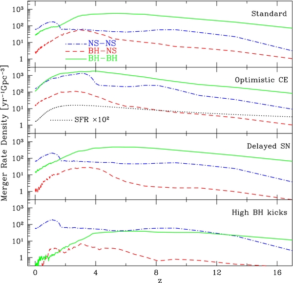
Figure 3. DCO merger rate densities in the rest frame (intrinsic), for high-end metallicity. Each panel shows a different model, as listed (for details, see Section 3.2). The dash–dotted, dashed, and solid lines represent NS–NS, BH–NS, and BH–BH systems, respectively. The dotted line in the second panel from the top represents the SFR (see Equation (1)) multiplied by a factor of 100 for clarity; it is in units of M☉/100 Mpc−3 yr−1. This figure demonstrates: (1) a clear domination of NS–NS systems for the Standard model for z ≲ 1.6, as these systems merge copiously in the relatively metal-rich, local universe, (2) significantly increased merger rates for the Optimistic CE model, where CE events on the HG are allowed, and (3) a drastic drop in rates for the High BH Kicks model.
Download figure:
Standard image High-resolution image
Figure 4. Merger rate density vs. redshift and metallicity: this figure shows how the total merger rate density as a function of redshift is built up from systems formed in different star forming conditions. Each line indicates the contribution to the total merger rate density from each of the listed metallicity bins, for the Standard model. The sum of these curves (and the low-metallicity curves not shown in this plot) reproduce the total merger rate density shown in the top panel in Figure 3. The top, middle, and bottom panels show rate densities for NS–NS, BH–NS, and BH–BH systems, respectively. The peak of the NS–NS systems merger rate density in the rest frame is composed mostly of system created in 0.75 Z☉ environments. For BH–NS systems, the peak arises from 0.25 Z☉ environments and for BH–BH systems the peak arises from 0.25 Z☉–0.1 Z☉ environments.
Download figure:
Standard image High-resolution image
Figure 5. DCO merger rate density in the rest frame (intrinsic), low-end metallicity. For low redshifts (z < 2), the low metallicity decreases the merger efficiency of NS–NS systems.
Download figure:
Standard image High-resolution image
Figure 6. Cumulative merger rates in the observer frame, high-end metallicity. Panels are organized as in Figure 3. For the Standard model, the merger rates of NS–NS systems dominate until redshift z ≈ 2.4. For the Optimistic CE model, the merger rates of NS–NS and BH–BH systems are very similar until redshift z ∼ 1, where BH–BH systems take over. For the Delayed SN model, this happens at redshift z ∼ 3. For the High BH Kicks model, the NS–NS systems dominate the merger rates at all redshifts.
Download figure:
Standard image High-resolution image
Figure 7. Cumulative merger rates in the observer frame, low-end metallicity. Low metallicity causes an overall decrease in merger rates of NS–NS systems when compared with the high-end case (see Figure 6).
Download figure:
Standard image High-resolution image
Figure 8. Distribution of total mass for the BH–BH system for all models, high-end metallicity. The distribution is presented for BH–BH merging in two redshift ranges: one clustered around z = 1 and one around z = 5 (each range spans 1 Gyr; the corresponding limiting redshifts are given in the bottom panel). The redshift values are chosen arbitrarily for illustrative purposes. Note that as the redshift decreases so does the maximum total mass of the system.
Download figure:
Standard image High-resolution image
Figure 9. Distribution of total mass for the BH–BH system for all models, low-end metallicity.
Download figure:
Standard image High-resolution image2. STELLAR POPULATIONS
In this section, we describe the properties of stellar populations and their evolution with redshift. The formalism is mostly adopted from Belczynski et al. (2010c).
2.1. Star Formation History
In order to determine the merger rates of DCOs, we need the star formation rate (SFR). We adopt the formula provided by Strolger et al. (2004):

where t is the age of the universe (Gyr) as measured in the rest frame, t0 is the present age of the universe (13.47 Gyr; see Section 4), and the parameters have values a = 0.182, b = 1.26, c = 1.865, and d = 0.071. The SFR described above is expressed in comoving units of length and time.
2.2. Galaxy Mass Distribution
For redshifts z < 4, we describe the distribution of galaxy masses using a Schechter-type probability density function, calibrated to observations (Fontana et al. 2006):

where Φ*(z) = 0.0035(1 + z)−2.2,  (Mz = 11.16 + 0.17z − 0.07z2), and α(z) = −1.18 − 0.082z. A galaxy mass is drawn from this distribution in solar units (M☉) and in the range 7 < log (Mgal) < 12. Beyond redshift z = 4, we assume no further evolution in galaxy mass, fixing the mass distribution to the value at z = 4. This assumption reflects the lack of information on galaxy mass distribution at high redshift.
2.3. Galaxy Metallicity
We assume the average oxygen-to-hydrogen number ratio (FOH = log (1012O/H)) in a typical galaxy to be given by

As suggested by Erb et al. (2006) and Young & Fryer (2007), the functional form of this mass–metallicity relation is redshift independent, with only the normalization factor s varying with redshift. We describe the redshift dependence of galaxy metallicity using the average metallicity relation from Pei et al. (1999):

which implies the evolution of s with redshift:

We assume that the oxygen abundance (used in FOH) correlates linearly with the average abundance of elements heavier than helium (encapsulated in the metallicity measure, Z).
In this paper, we employ two distinct scenarios for metallicity evolution with redshift in order to investigate the uncertainties of the chemical evolution of the universe. The construction of these scenarios consists of several steps. (1) We utilize two normalizations of Equation (3). In the first, provided by Pei et al. (1999), the coefficients are a2 = 0.5, b1 = 0.8, b2 = 0.25, c1 = 0.2, and c2 = 0.4. This grants a rate of average metallicity evolution, which we label slow. The second, provided by Young & Fryer (2007), uses a2 = 0.12, b1 = −0.704, b2 = 0.34, c1 = 0.0, and c2 = 0.1992. It is based on ultraviolet Galaxy Evolution Explorer, Sloan Digital Sky Survey (SDSS), and Spitzer infrared and Super Kamiokande neutrino observations (Hopkins & Beacom 2006). This normalization produces a faster rate of chemical evolution and we label the results fast. At this point, for each galaxy mass value at a given redshift (Equation (2)), we have two metallicity values (Equation (3)). (2) We then combine these (slow and fast) metallicities into a single value that is an average of the two; we label this profile as initial. However, this profile yields an unrealistically high number of galaxies with extrasolar (up to 3 Z☉; Z☉ = 2% of stellar mass) metallicities at redshift z ∼ 0. (3) In order to be consistent with observational data, we scale down the profile so that it agrees with the observed metallicities of galaxies in the local universe (at z ∼ 0). We explore two such "extreme" scalings resulting in a pair of final metallicity evolution profiles. In the first, we divide the metallicity values from the initial profile by a factor of 1.7. This produces a median value of metallicity of 1.5 Z☉ at z ∼ 0 (see Figure 1), which corresponds to 8.9 in the "12+log(O/H)" formalism. This calibration was designed to match the upper 1σ scatter of metallicities according to Yuan et al. (2013) (see their Figure 2, top-right panel). We label this profile as high-end, as it is the upper limit on metallicity at z ∼ 0. In the second, we utilize SDSS observations (Panter et al. 2008), from which we infer that one half of the star forming mass of the galaxies at z ∼ 0 has 20% solar metallicity, while the other half has 80% solar metallicity. This yields a median metallicity value of 0.8 Z☉ and requires the division of the initial profile by a factor of three. We label this profile as low-end.
2.4. Galaxy Stellar Populations
We distinguish three stellar populations:

We choose FOH, gal = 10−4 as the delineation point between Population II and III stars. A lower abundance of metals provides insufficient cooling in the collapse of gas clouds and thus significantly alters the star formation for Population III stars (e.g., Mackey et al. 2003; Smith et al. 2009). The border point between Population II and I stars is dictated by observations in the Milky Way (e.g., Binney & Merrifield 1998; Beers & Christlieb 2005).
We assume that the binary fraction is 50%: for each single star, there exists one binary. We additionally assume that all the stars within each galaxy share the same metallicity value. The use of average metallicity seems to be appropriate since we draw a large (104) number of galaxies (Equation (2)) via Monte Carlo simulations.
3. BINARY STAR MODELING
We present our calculations for a set of 4 models, each differing in major input physics (see Table 1 and the subsequent sections). For each model, we use a grid of 11 metallicity values (Z = 0.03, 0.02(solar,Z☉), 0.015, 0.01, 0.005, 0.002, 0.0015, 0.001, 0.0005, 0.0002, 0.0001) in order to accurately account for the average metallicity evolution of the stellar populations with redshift.
3.1. The StarTrack Code
To calculate the evolution of the stellar populations, we utilize the recently updated (Belczynski et al. 2010a, 2012; Dominik et al. 2012) Startrack population synthesis code (Belczynski et al. 2002, 2008). This code can evolve isolated binary stars that are interacting in quasi-hydrostatic equilibrium from the zero-age main sequence (ZAMS), through mass transfer, to the formation of compact objects and to the ultimate merger of the binary components. The code makes use of an extensive set of formulae and prescriptions that adequately approximate more detailed binary evolution calculations (see Hurley et al. 2000).
StarTrack allows one to investigate stable and unstable mass transfers between the binary components. Stable transfer calculations have been calibrated on massive binaries that are relevant to DCO formation (e.g., Tauris & Savonije 1999; Wellstein et al. 2001). It is yet unknown exactly how conservative the stable mass transfer is. Dewi & Pols (2003) suggest that in massive binaries the fraction of the envelope of the donor accreted by its companion ranges between 40% and 70%. In our calculations, we fix this value to be 50% or, in mathematical terms:

where  is the accretion rate,
  is the mass transfer rate from the donor, and fa is the fraction of the rate transferred (here equal to 0.5). The remaining mass is expelled to infinity. The dynamically unstable mass transfers (CE) is calculated according to the energy balance formula (Webbink 1984), with the envelope binding energy parameter λ adopted from Xu & Li (2010).
Tidal interactions and their influence on eccentricity, the semi-major axis, and rotation is also evaluated. The calculations are done with the standard equilibrium-tide, weak-friction approximation (Zahn 1977, 1989), using the formalism of Hut (1981). However, the code does not allow one to investigate the influence that rotation of the components has on the internal structure of the components.
Stellar winds are taken into account as a function of the metallicity and evolutionary stage of the star. This piece of physics is especially important as it has a significant impact on the masses of remnant objects, which are the centerpiece of this study. In short, the wind mass loss rates are divided into categories specific to the evolutionary stage of the star: O/B–type, red giant, asymptotic red giant, Wolf–Rayet stars, and luminous blue variable (LBV) stars. The magnitude of the rates increases with metallicity of the star except for the LBV phase. In this stage, the winds are set to be of the order of 10−4 M☉ yr−1. This value was calibrated to account for the highest mass BHs in the Milky Way ∼15 M☉ (Cyg X-1 and GRS 1915). A detailed description of wind mass loss rates can be found in Belczynski et al. (2010a).
Besides stellar winds, the code also calculates changes of the angular momentum arising from gravitational radiation and magnetic braking. The latter is adopted from Ivanova & Taam (2003).
Additionally, the code utilizes the convection-driven, neutrino-enhanced SN engines (Fryer et al. 2012) to determine the properties of the remnant objects (neutron stars (NSs) and BHs).
For each metallicity value in each model, we evolve 2 × 10⁶ binaries, assuming that each component is created at the same time. Each binary system is initialized by four parameters that are assumed to be independent. These are: primary mass, M1 (initially more massive component), mass ratio, q = M2/M1, where M2 is the mass of the secondary component (initially less massive), the semi-major axis, a, of the orbit, and the eccentricity, e. The mass of the primary component is randomly chosen from the initial mass function adopted from Kroupa et al. (1993) and Kroupa & Weidner (2003):

where α = 2.7 is our standard choice for field populations. The choice of the upper initial mass function (IMF) cutoff (150 M☉) is justified by observations of massive stars in the Milky Way (Figer 2005; Oey & Clarke 2005). Stars are generated from within an initial mass range, with the limits based on the targeted stellar population. For example, studies of single NSs require their evolution within the range 8–20 M☉, while for single BHs the lower limit is 20 M☉. Binary evolution may broaden these ranges due to mass transfer episodes and we therefore set the minimum mass of the primary to 5 M☉. We assume a flat mass ratio distribution, Φ(q) = 1, over the range q = 0–1, in agreement with recent observations (Kobulnicky & Fryer 2007). Given a value of the primary mass and the mass ratio, we obtain the mass of the secondary from M2 = qM1. However, for the same reasons as for the primary, we do not consider binaries where the mass of the secondary is below 3 M☉. The distribution of initial binary separations is assumed to be flat in log (a) (Abt 1983) and so ∝1/a, with a ranging from values such that at ZAMS the primary fills no more than 50% of its Roche lobe to 105 R☉. For the initial eccentricity, we adopt a thermal equilibrium distribution (e.g., Heggie 1975; Duquennoy & Mayor 1991): Ξ(e) = 2e, with e ranging from 0 to 1. We find that the adopted parameters are in accordance with the most recent observations of O-star populations (Sana et al. 2013).
3.2. The Model Suite
3.2.1. The Standard Model
In this subsection, we define a reference model for this paper. This model is identical to the "Standard model–submodel B" in the previous paper in this series (Dominik et al. 2012).
The list of major parameters describing the input physics of binary evolution in this model begins with the Nanjing λ (Xu & Li 2010) CE coefficient used in the energy balance prescription (Webbink 1984). This λ value depends on the evolutionary stage of the donor, its mass at ZAMS and the mass of its envelope, and its radius. In addition, all of these quantities depend on metallicity, which in our simulations changes within a broad range (Z = 10−4–0.03).
However, before calculating the aforementioned energy balance to determine the outcome of the CE, we check the evolutionary type of the donor star. For example, main sequence (MS) stars do not have clear core-envelope division, as the helium core is still in the process of being developed. Donors on the HG behave similarly, although it remains unclear if such a division can appear on the HG or not until later stages, like the core helium burning stage (P. Eggleton 2010, private communication). In our previous work, we investigated two possibilities of the CE outcome associated with the type of the donor star: an automatic (premature) merger if the donor is an HG star, regardless of the energy balance (labeled as "submodel B") or allowing the CE energy balance to unfold ("submodel A").
The case in which we allow for potential survival of systems with HG donors results in very high Advanced LIGO/VIRGO detection rates (∼8000 yr−1; Belczynski & Dominik 2012), exceeding even the empirically estimated rates based on IC10 X-1 and NGC 300 X-1 (∼2000 yr−1; Bulik et al. 2011; Belczynski et al. 2013). Therefore, we only show one model with this generous assumption on CE physics, which leads to the most optimistic of our predictions. This model (Optimistic CE) will be tested (and probably quickly eliminated) by the upper limits from the Advanced LIGO/VIRGO engineering runs. For all the other models, including our reference model, we make the conservative assumption that none of the HG donor CE phases lead to the formation of DCOs.
Observations suggest (Hobbs et al. 2005) that NSs formed in SNe receive natal kicks, with velocities drawn from a Maxwellian distribution with σ = 265 km s−1. We employ these findings in our simulations and extend them so that BH natal kicks match this distribution as well. However, it is possible that some matter ejected during the explosion will not reach the escape velocity and will thus fall back on the remnant object, potentially stalling the initial kick. To account for this process, we modify the Maxwellian kicks by the amount of matter falling back onto the newly formed compact object:

where Vk is the final magnitude of the natal kick, Vmax is the velocity drawn from a Maxwellian kick distribution, and ffb is the fallback factor describing the fraction of the ejecta returning to the object. The values of ffb range between 0–1, with 0 indicating no fallback/full kick and 1 representing total fallback/no kick (a "silent supernova," e.g., Mirabel & Rodrigues 2003). We label this the "constant velocity" formalism. An alternative approach is the "constant momentum" formalism, where the kick velocity is inversely proportional to the mass of the remnant object. In general, constant velocity provides larger natal kicks on average than constant momentum, resulting in more frequent disruptions of binaries, especially for systems with BHs. Therefore, we choose the "constant velocity" formalism over the "constant momentum" as it provides a more conservative limit on the number and therefore merger rates of systems containing BHs.
This model also utilizes the "Rapid" convection-driven, neutrino-enhanced SN engine (Fryer et al. 2012). It allows for a successful explosion without the need for the artificial injection of energy into the exploding star. In this scenario, the explosion starts from the Rayleigh–Taylor instability and occurs within the first 0.1–0.2 s. For low-mass stars (Mzams ≲ 25 M☉), the result is a very strong (high-velocity kick) SN, which generates an NS. For higher mass stars, a BH is formed through a direct collapse (a failed SN). This engine, incorporated into binary evolution, successfully reproduces the mass gap (Belczynski et al. 2012) observed in Galactic X-ray binaries (Bailyn et al. 1998; Özel et al. 2010).
The list of major physical parameters used in this and subsequent models is given in Table 1. More details on the physics described above can be found in Dominik et al. (2012).
3.2.2. Variations on the Standard Model
The uncertainties in the CE and the SN engine argue for exploring a range of input physics beyond that in the Standard model described in the previous subsection. In this subsection, we present three additional models that we have found to encapsulate the full range of possible binary evolutions. All subsequent models use the same input physics as the reference model, except for the parameters described below.
Optimistic Common Envelope. In this model, we allow HG stars to be CE donors (see Section 3.2.1). When the donor initiates the CE phase, the energy balance determines the outcome. This model is identical to the "Standard model–submodel A" from our previous paper in this series (Dominik et al. 2012).
Delayed Supernova. This model utilizes the "Delayed" SN engine instead of the Rapid one. The Delayed is also a convection-driven, neutrino-enhanced engine, but is sourced from the standing accretion shock instability and can produce an explosion as late as 1 s after bounce. The Delayed engine produces a continuous mass spectrum of compact objects, from NSs through light BHs to massive BHs (see Belczynski et al. 2012). This model is identical to the "Variation 10–submodel B" model from our previous paper in this series (Dominik et al. 2012).
High BH Kicks. In this model, the BHs receive full natal kicks. The newly formed BH acquires a velocity drawn from a Maxwellian distribution (see Section 3.2.1) regardless of the fallback factor ffb (see Equation (9)). This model is identical to the "Variation 8–submodel B" model in our previous paper in this series (Dominik et al. 2012).
4. COSMOLOGICAL CALCULATIONS
We utilize a flat cosmology with H0 = 70 km s−1 Mpc−1, ΩM = 0.3, ΩΛ = 0.7, and Ωk = 0.0. The relationship between redshift and time is given by

where tH = 1/H0 = 14 Gyr is the Hubble time (e.g., Hogg 1999) and  .
.
The comoving volume element dV is given by

where c is the speed of light in vacuum, dΩ is the solid angle, and Dc is the comoving distance given by

There are a series of steps to calculate the rates of events, as we now describe. We employ time as our reference coordinate and start by creating time bins across the entire history of universe, each bin 100 Myr wide, from 0.13 Gyr (birth) to 13.47 Gyr (today). At the center of each bin, we evaluate the SFR according to Equation (1). For the redshift value corresponding to the center of a given time bin, we generate a Monte Carlo sample of 104 galaxies (a number sufficient to produce a smooth distribution) with masses drawn from the distribution given in Equation (2). For each time bin, we obtain a total mass of galaxies Mgal, tot. For each galaxy, we then estimate its average metallicity using Equation (3). We assume that all stars within a given galaxy have identical metallicity, as obtained from Equation (3). Since we draw a large number of galaxies in each time bin and each galaxy has its own mass and therefore is described by its own average metallicity, we end up with a distribution of metallicity in each time bin. This also yields a total mass of galaxies with a specific metallicity (Mgal, i) within each time bin. We then define the fraction of the total galaxy mass capable of forming stellar population with a specific metallicity by

However, because we use a finite number of metallicity points in our simulations (see Section 3), we need to extrapolate our results in order to account for the continuous spectrum given by Equation (3). Therefore, the metallicity points are extended into bins delineated by the average value of neighboring points. For example, given the set of points Z = 0.01, 0.015, and 0.02, the value Z = 0.015 now corresponds to a bin that extends from 0.0125 to 0.0175. The border points Z = 0.0001 and Z = 0.03 extend to lower and higher values, respectively, to cover the rest of the spectrum.
Population synthesis provides us with a representative sample of DCOs. The formation of a single DCO within a time bin corresponds to a fraction, ffr, of the total formation rate:

where Msim is the total mass in our population synthesis calculations (see Section 3). Repeating this calculation of ffr for each metallicity yields a total formation rate, ffr, tot, within a given time bin.
We now need to know the delay time until the merger, tdel, for each DCO formed. The delay time is defined as the interval between the formation of the progenitors of a DCO and the coalescence of two compact objects. For each DCO originating from a specific metallicity, we randomly choose a birth point, t0 (ZAMS), within each time bin. We then propagate the system forward in time toward its merger using the delay time:

As long as we consider DCOs with tmer < tH and as long as the width of the time bins throughout the time line is constant, the formation rate (ffr) of a DCO from a given bin translates into a merger rate in a later bin, propagated forward in time by tdel. Repeating the above calculations for every time bin yields a total density of rest-frame merger events, nrest(t), in units of Gpc−3 yr−1. In other words

where i sums over each representative DCO.
5. RESULTS
We now provide results from our four models, presenting the intrinsic merger rate densities and the observer-frame merger rates, given by

with dV/dz given by Equation (11), integrated over the solid angle dΩ (hence the factor of 4π). In the case of the Standard/reference model (details in Section 3.2.1), we explain the general redshift behavior of all three types of DCOs (NS–NS, BH–NS, and BH–BH) and compare the reference model for two scenarios of metallicity evolution (high-end and low-end). For our three variations (Optimistic CE, Delayed SN, and High BH kicks; Section 3.2.2), we investigate deviations from the reference model, again incorporating our different metallicity evolutionary scenarios.
5.1. Standard Model
NS–NS. As shown in Figure 3, the intrinsic merger rate densities of double NS systems peak at redshift z ≈ 1 (∼200 yr−1 Gpc−3). As a general rule, the merger rates of all types of DCO are directly related to the SFR. However, for a given SFR value, the formation efficiency of different DCOs may vary. In other words, the proportions of NS–NS, BH–NS, and BH–BH systems may differ beyond the regime set by the IMF (e.g., Dominik et al. 2012). For example, NS–NS systems are on average efficiently created in high-metallicity environments (see Figure 4). When combined with the peak of the SFR at z ∼ 2 (the average high-end metallicity is ∼0.4 Z☉; see Figure 2), high-metallicity NS–NS formation efficiency is enhanced, thus creating the profile shown in Figure 3. What is characteristic for this profile is the "hump" that arises at z ∼ 1.6, approaching from high redshifts. As can be seen in Figure 4, this shape is dominated by mergers originating from 0.75 Z☉ environments. The reason for this increase in merger rate densities, when transiting from 0.5 Z☉ environments (higher redshifts) to higher metallicity ones (lower redshifts), is a consequence of the applied CE approach. Within the framework of the Nanjing CE treatment adapted for the Startrack code, the binding energy of the CE decreases at the 0.5–0.75 Z☉ boundary, allowing for the survival of a larger number of NS–NS progenitors.
In comparison, for the low-end metallicity profile, the NS–NS systems dominate the rates only up to z ≈ 0.5 (Figure 5). This is a consequence of the adopted metallicity evolution scenario. Specifically, galaxies of a given metallicity are shifted to lower redshift when compared with the high–end scenario, causing a shift of the NS–NS systems also to lower redshifts.
As shown in Figure 6, in the observer frame the systems dominate the merger rates up to redshift z ≈ 2.4. However, decreased metallicity for the low-end case shifts this point to z ≈ 0.6 (Figure 7).
BH–NS. For the high-end metallicity evolution, the rest-frame merger rate densities for BH–NS systems shown in Figure 3 peaks at a value of ∼50 Gpc−3 yr−1 at redshift z ∼ 3. However, the merger rate efficiency drops for low (z ∼ 0) and high (z ∼ 6) redshifts. This is because of properties of the progenitor masses. For metallicities ∼Z☉, the bulk of the progenitors masses are in the range 45–60 M☉ for the primary component and 22–32 M☉ for the secondary. Pairs of progenitors outside these ranges are unlikely. The upper mass limit delineates between BH–NS and BH–BH systems; crossing it results in the formation of the latter systems instead of the former. The lower mass limit is set by a similar phenomenon, only this time through BH–NS/NS–NS formation. Progenitors of these systems for metallicities a factor of ∼10 lower than Z☉ must have lower masses on average, primarily because of the decreased stellar wind mass losses. Otherwise, the binary would retain enough mass to form a BH–BH system or go through a terminal CE event. Therefore, the mass ranges for BH–NS progenitors for Z ∼ 10% Z☉ are 20–50 M☉ for the primary and 12–25 M☉ for the secondary. Given that in this mass range the IMF scales as M−2.7 (where M is the mass of the progenitor), there are more BH–NS progenitors available at moderately low metallicity than at higher values. This, in turn, translates into increased merger rates arising from these environments. Decreasing the metallicity to ∼1% Z☉ decreases the masses of the progenitors even further due to the same wind effects. However, in this case the BH progenitors are closely approaching their lower mass limit (∼20 M☉), which leaves a narrow mass range: 20–25 M☉ for the primary and 18–22 M☉ for the secondary. There are fewer progenitors in these mass ranges when compared with the previous case and therefore we find a lower merger rate. Overall, the BH–NS merger rates peak originates from systems being created at moderate metallicities (see Figure 4).
BH–BH. For these systems, the intrinsic merger rate has a peak-plateau at a rate of ∼300–400 Gpc−3 yr−1 at z ∼ 4–8, for the high-end case. The low-metallicity galaxies abundant at high redshifts are efficient BH factories (see Figures 8 and 9). This also means that adopting the low-end metallicity scenario will allow for more BH–BH systems to form at lower redshifts, when compared with the high-end. Additionally, environments with low amounts of metals favor massive BHs. For example, the most massive BH–BH system acquired in this model consisted of a 62 M☉ and a 74 M☉ BH pair. These systems originate from the extremely low metallicity environments (Z = 0.0001). We find that such systems merge up until redshift z ∼ 3 and z ∼ 2 for the high-end and low-end metallicity evolution models, respectively. However, due to statistical uncertainties, these redshift values may be even lower. These massive systems originate through the standard BH–BH formation channel. As an instructive example, we detail the formation scenario of an 8.3–5.8 M☉ BH–BH, for Z = 0.005—a typical system for the average metallicity acquired in our study: t = 0 Myr. The components start with masses 32 M☉ and 25 M☉ for the primary and secondary, respectively, and an orbital separation a = 995 R☉. t = 6.7 Myr. The primary, after becoming an HG star, expands and initiates a mass transfer through Roche lobe overflow (RLOF). The transfer continues until the primary loses almost all of its hydrogen envelope and becomes a Wolf–Rayet star with 10 M☉ (the secondary component has 35 M☉). The orbital separation prior to RLOF was a = 1000 R☉ and a = 1600 R☉ after t = 7.0 Myr. The primary explodes as an SN, forming a 7.8 M☉ BH. The orbital separation after the explosion was a = 1760 R☉ t = 8.7 Myr. The secondary (34 M☉) initiates a CE phase and becomes a Wolf–Rayet star with 11 M☉ as a result of the outcome (the primary gained ∼0.5 M☉). The orbital separation prior to the CE was a = 1780 R☉ and a = 2.6 R☉ after t = 9.4 Myr. The secondary undergoes an SN and becomes a 5.8 M☉ BH. The orbital separation prior to the explosion was a = 2.8 R☉ and a = 3 R☉ after t = 26 Myr. The coalescence of an 8.3 M☉–5.8 M☉ BH–BH system occurs. This example is illustrated by a diagram in Figure 10.

Figure 10. Evolutionary diagram illustrating the example in Section 5.1, BH–BH paragraph. MS–main sequence, HG–Hertzsprung gap, CHeB–core helium burning, WR–Wolf–Rayet. From the top: I panel: progenitors at ZAMS, II panel: non-conservative, stable mass transfer from an HG donor (primary) to the companion, III panel: a WR star prior to an SN explosion (primary) and a rejuvenated companion, IV panel: CE event with a CHeB donor (secondary) and a BH accretor (primary), V panel: the binary immediately after the CE, and VI panel: the formation of a BH–BH system.
Download figure:
Standard image High-resolution image
On a side note, the formation of the most massive BH–BH systems on close orbits may be questionable. The progenitors of the aforementioned 62 M☉–74 M☉ BH–BH system are massive stars (140 M☉–150 M☉ at ZAMS). A recent theoretical study by Yusof et al. (2013) suggests that such objects (150 M☉–500 M☉) will not increase in size significantly during their evolution. Therefore, it is more likely for such binaries to bypass the CE phase and avoid the reduction of orbital separation. This in turn will prevent the resulting BH–BH system from merging within a Hubble time.
In the observer frame, BH–BH systems begin to dominate the merger rates at z ∼ 2. For the low-end case, this happens closer to z ∼ 1.
5.2. Optimistic CE
In this model, we relax one of the conditions on CE survivability. Specifically, HG donors are now allowed to undergo full energy balance calculations. In the Standard model, CEs with HG donors resulted in an immediate merger, terminating further binary evolution. This has been shown to have a significant impact on the number of DCOs, altering the merger rates by orders of magnitude (Belczynski et al. 2007, 2010b). When HG donors survive CE, their numbers naturally increase, as do their merger rates.
NS–NS. When compared with the Standard model, the high-end case, the intrinsic merger rate of NS–NS systems peaks at higher redshift (z ∼ 3) and at higher values (∼1000 Gpc−3 yr−1). The shift in the peak toward higher redshifts is associated with the systems having shorter delay times on average, which allows them to merge more quickly after formation. As expected, the decrease of average delay times for NS–NS systems is caused by the new CE condition. In the Standard model, the only surviving binaries were those that did not initiate the CE while the potential donor was an HG star. In order to prevent a rapidly expanding HG star from overfilling its Roche lobe, these binaries had to have a significant initial separation, which resulted in relatively large delay times. In this model, the CE phase with an HG donor is allowed, so initial separation is no longer such a crucial issue. Therefore, binaries with smaller initial separations are able (if they have sufficient orbital energy) to survive and form NS–NS systems. This results in shorter delay times. In the low-end case, the same mechanism causes the peak to shift toward z ∼ 2.
In the observer frame, the merger rate of NS–NS systems is a few times higher than in the Standard model for both high-end and low-end metallicity evolutions. In the former case, NS–NS systems dominate the merger rates up to z ≲ 0.5. In the latter case, they are always sub-dominant compared with BH–BH systems.
BH–NS. The binaries forming these systems usually undergo two CE events in their lifetimes, due to their relatively high initial mass ratios (for details, see Dominik et al. 2012). The two CEs reduce the initial separation, which makes the relaxed CE condition much less relevant than for the NS–NS case discussed above. The result is that there are no significant changes in the intrinsic merger rate density for BH–NS systems. As in the Standard model, the mergers of BH–NS systems are the rarest of all types of DCOs. This is true for both of the metallicity scenarios.
BH–BH. These systems do not experience two CE events, unlike the BH–NS systems and therefore they do not reduce their initial separations as efficiently. The peak of the intrinsic merger rate density shifts slightly toward lower redshift (z ∼ 4; high-end) when contrasted with the reference model (see Figure 3). This is because of the effect of metallicity on the outcome of the CE phase. The larger the fraction of metals in a star, the bigger its radius (e.g., Hurley et al. 2000). This effect is particularly strong during the HG phase. Therefore, high-metallicity BH progenitors are more likely to initiate CE on the HG. In the Standard model, this is not allowed and such systems are removed from the population. However, here we relax this condition and as a consequence we add more BH–BH systems originating from higher metallicities (see Figures 8 and 9). For the low-end case, this results in a peak-plateau between redshifts 3 < z < 4. This is because of the higher metallicities appearing at lower redshifts when compared with the high-end case.
In the observer frame, the BH–BH systems start to dominate the merger rates at z ≈ 0.5 in the high-end case. For the low-end case, these DCOs are always primary mergers.
5.3. Delayed SNe
In this model, we change the SN explosion engine with respect to the Standard model. The Standard model uses the Rapid engine, which yields a gap between 2–5 M☉ in the masses of the resulting compact objects. Here, we utilize the Delayed scenario (for details, see Section 3.2.2). The main feature of this engine is that it produces a continuous mass spectrum of remnant objects (Belczynski et al. 2012). As suggested by Kreidberg et al. (2012), the presence of the mass gap feature may be a result of systematic errors arising from misinterpretation of the BH binary light curve analyses. The resulting errors in estimating the inclination of the binary may shift low-mass BHs from the gap. The distinction between the two engines is clearly visible in Figures 8 and 9. The minimal total mass for this model is ∼5 M☉. Such a system is composed of two BHs of 2.5 M☉ each (2.5 M☉ being the delineation between upper NS and lower BH mass). For other models, the minimal BH mass is ∼5 M☉, thus yielding a minimal total mass ∼10 M☉. However, the SN engine effects do not play a significant role in the merger rates of any type of DCOs.
5.4. High BH Kicks
Here, we employ full natal kicks (as measured for NSs) just on BHs (see Section 3.2.2). This is performed regardless of the amount of fallback (see Equation (9)). The kicks for NS–NS systems remain unchanged, as does their population with respect to the Standard model.
In this variation, the velocity of the natal kick acquired upon BH formation will disrupt many binaries that would otherwise (in the Standard model) form coalescing BH–NS or BH–BH systems, as is clearly visible in Figure 3. As a consequence, the NS–NS systems will dominate the merger rates in the observer frame.
In addition, the full natal kick will affect the most massive BHs. In the Standard model, stars with masses Mzams > 40 M☉ would collapse directly into a BH after the SN explosion; with no asymmetric ejecta, they do not receive a kick (ffb = 1, Equation (9)). However, in this model, these stars receive a maximum velocity kick and thus often disrupt the system. As a consequence, the probability of the formation and eventual merger of the most massive BH–BH systems is lowered significantly, which can be seen in the bottom panel of Figures 8 and 9.
6. SUMMARY AND DISCUSSION
We have performed a series of cosmological calculations for four populations of DCOs. Each population was generated with different input physics for describing binary evolution and compact object formation. The first model (the Standard model) utilizes the current state-of-the-art description of physical mechanisms governing DCOs. In particular, it uses a Rapid explosion engine, which yields results accurately describing the mass distribution of X-ray binaries (see Section 3.2.1, and references therein). Another major improvement in the model is the realistic treatment of the CE parameter λ, which now depends on the evolutionary stage, radius, mass, metallicity, etc. of the donor star. The three subsequent models explore alternative outcomes of binary evolution and the resulting properties of remnants. The mechanisms investigated in these models are the sensitivity of the CE outcome to the type of donor, the Delayed SN explosion mechanism, and the natal kick survivability of DCOs containing BHs (see Section 3.2.2). Additionally, for each model, we created a grid of 11 metallicities to account for the chemical evolution throughout the lifetime of the universe. We present both the intrinsic and the observer-frame merger rates as a function of redshift.
The variation in the rates of our different binary systems as a function of redshift depends upon metallicity, as well as CE and SN physics. In this paper, we have studied how these impact the rates for different types of DCOs. Here, we review our main findings.
We find that NS–NS systems merge most efficiently at low redshifts (z ≲ 1; see Figures 3 and 5), where metallicities become relatively high (∼0.5 Z☉). However, in the case of the Optimistic CE model, the merger rate densities peak at higher redshifts (z ∼ 2–3). This results from relaxing the condition for the termination of binaries initiating a CE with an HG donor. This Optimistic CE treatment enriches the merging population with systems with short merger times. As a result, the overall number of NS–NS systems increases and, due to the shorter merger times, these systems coalesce earlier (see Sections 3.2.2 and 5.2).
BH–NS systems merge most infrequently in all but one of the models. The exception is the Full BH Kicks model, where full natal kicks are applied to BH remnants. The kicks eliminate binaries containing BHs from the populations by disrupting them. However, this does not affect BH–NS systems as strongly as BH–BH systems since the former systems contain only one BH. In general, the low merger rates of BH–NS systems arise from their unique mixed nature. Forming two different compact objects in a single binary generally requires the masses of the progenitors to be significantly separated. This plays an important role at first contact between the components, since if the mass ratio of the binary is larger than 2–3 the otherwise-stable mass transfer through RLOF may become a CE event. These episodes often cause a premature merger and eliminate further binary evolution. Another important factor in making the BH–NS systems small in numbers is that the progenitors do not have a large range of masses to draw from. The upper limit is set by the binary containing enough mass to form a BH–BH system instead, while the lower limit is set by not having enough mass and instead forming an NS–NS system.
For BH–BH systems, the highest merging efficiency occurs earlier in the universe when compared with other DCOs (z ∼ 4–6). This arises from the fact that these systems form most efficiently at the lowest metallicities. For any of the two scenarios of metallicity evolution, the Optimistic CE model blurs this trend. In this case, the population is enriched by BHs, which originated from high-metallicity environments (see Section 5.2). Another interesting case is the model with High BH Kicks, where BH–BH systems are efficiently disrupted by natal kicks throughout the lifetime of the universe. This is clearly visible in the bottom panel of Figures 3 and 5. The kicks affect high-mass systems the most. As a consequence of the full natal kicks, the formation and merger rates for BH–BH systems in low-metallicity galaxies (higher redshifts) are reduced significantly and this effect is even more dramatic for high-metallicity environments (lower redshifts; see Figures 8 and 9). The High BH Kicks model produces a difference between the merger rates in the observer frame of BH–BH and NS–NS systems that is roughly 100 times larger than within the Standard model. This may be a promising avenue for determining the magnitude of the natal kicks imparted to BHs during their formation.
Since (only) NS–NS systems have been observed, we can use observed rates to put constraints on our models. The NS–NS merger rates in each of our models, at z ∼ 0, fit within the observational limits for NS–NS systems in the Milky Way: 34.8–2204 yr−1 Gpc−3 (Kim et al. 2006), using the galaxy density ρgal = 0.0116 Mpc−3. Petrillo et al. (2013) used the observed rate of short GRBs to calculate the merger rates of NS–NS and BH–NS systems, since these systems are thought to be the progenitors of short GRBs. The resulting merger rates of DCOs (NS–NS + BH–NS) in the local universe ranges between 500 and 1500 Gpc−3 yr−1. At z ∼ 0, our models find an NS–NS merger rate of ∼100 Gpc−3 yr−1, with a BH–NS rate lower by a factor of ∼10. However, the authors of the aforementioned study state that their results are sensitive primarily to the poorly constrained beaming angle of the colimated emission from short GRBs. They used a beaming angle of ∼20°, while to match our rate the beaming angle would have to be ∼50° (see Figure 3 therein). In our previous study (Dominik et al. 2012), we found one model that would reproduce the merger rates of NS–NS + BH–NS from Petrillo et al. (2013) (∼900 Gpc−3 yr−1 at Z☉). It is the model described by fully conservative mass transfer episodes and an Optimistic CE description (labeled "Variation 12–submodel A").
Additional constraints may be provided by observing the potential electromagnetic signatures, other than GRBs, of DCO mergers. One example is the optical/radio afterglow of the GRB, which can be detected even if the GRB itself is not seen (an "orphan afterglow"). Another possibility is a "kilonova," resulting from the ejection of matter from an NS. Since this matter may be enriched in heavy elements through the r-process, the resulting radioactive decay may generate observable light, thereby providing a promising electromagnetic counterpart to the GW emission (Metzger & Berger 2012; Piran et al. 2013; Barnes & Kasen 2013).
Finally, it will be interesting to investigate how statistical ensembles of GW observations can constrain properties of compact binary populations and of their formation scenarios (see, e.g., Mandel 2010; O'Shaughnessy 2012; Gerosa et al. 2013).
We thank Alexander Heger for a helpful discussion on pair–instability supernovae. We also thank the N. Copernicus Astronomical Centre in Warsaw, Poland and the University Of Texas, Brownsville, TX, for providing computational resources. D.E.H. acknowledges support from National Science Foundation CAREER grant PHY-1151836. K.B. and M.D. acknowledge support from MSHE grant N203 404939 and N203 511238, NASA Grant NNX09AV06A to the UTB, Polish Science Foundation Master 2013 Subsidy and National Science Center DEC-2011/01/N/ST9/00383. T.B. was supported by the DPN/N176/VIRGO/2009 grant. E.B. acknowledges support from National Science Foundation CAREER grant No. PHY-1055103. Work by C.L.F. was done under the auspices of the National Nuclear Security Administration of the U.S. Department of Energy under contract No. DE-AO52-06NA25396.