


ABSTRACT
We present new Hubble Space Telescope observations of H i Lyα absorption toward the F8 V star HD 35296. This line of sight is only a few degrees from the downwind direction of the local interstellar medium flow vector. As a consequence, Lyα absorption from the heliotail is detected in the spectrum, consistent with three previous downwind detections of heliotail absorption. The clustering of the heliotail absorption detections around the downwind direction demonstrates that the heliotail is pointed close to that direction, limiting the extent to which the interstellar magnetic field might be distorting and deflecting the heliotail. We explore this issue further using three-dimensional MHD models of the global heliosphere. The three computed models represent the first three-dimensional MHD models with both a kinetic treatment of neutrals and an extended grid in the tail direction, both of which are necessary to model Lyα absorption downwind. The models indicate only modest heliotail asymmetries and deflections, which are not large enough to be inconsistent with the clustering of heliotail absorption detections around the downwind direction. The models are reasonably successful at reproducing the observed absorption, but they do overpredict the Lyα opacity by a factor of 2–3. We discuss implications of these results in light of observations of the heliotail region from the Interstellar Boundary Explorer mission.
Export citation and abstract BibTeX RIS
1. INTRODUCTION
In the classical picture of the heliosphere, the solar wind is slowed to subsonic speeds at a termination shock (TS) that is symmetric about an axis defined by the interstellar flow vector, and then the post-TS wind is deflected into a heliotail that points directly downwind relative to the interstellar medium (ISM) flow, bounded by a heliopause (HP) separating the solar wind and ISM plasma flows that is also symmetric about the ISM flow axis (Baranov et al. 1971; Holzer 1989; Zank 1999). This simple picture assumes that the interstellar magnetic field, BISM, is either insignificant or oriented parallel to the ISM flow. Although the potential importance of the ISM magnetic field in shaping the heliosphere has been recognized from the earliest heliospheric models (Parker 1961), poor knowledge of its characteristics prevented a detailed assessment of how significant the ISM field is for heliospheric structure.
Important constraints on the direction of BISM come from observations of interstellar hydrogen and helium flowing through the solar system (Lallement et al. 2005). Utilizing SOHO/SWAN data, Lallement et al. (2010) quote an ISM flow direction from ecliptic coordinates of (λe, βe) = (252 5, 89) for H, compared with (λe, βe) = (2554, 52) for He, indicating a deflection of H. The deflection of hydrogen is due to charge exchange processes, which change the character of H atoms as they flow through the heliosphere, in contrast to neutral He, which remains relatively unaltered. The direction of deflection of H is believed to be indicative of the orientation of the ISM magnetic field, so it is generally assumed that the field lies within the plane defined by the deflection direction, known as the hydrogen deflection plane (HDP).
Observations from the two Voyager spacecraft and from the Interstellar Boundary Explorer (IBEX) mission have provided additional valuable constraints on BISM. Voyager observations of the Lyα background and 2–3 kHz emission from the distant heliosphere have provided some indication of heliospheric asymmetry in the nose region (Ben-Jaffel et al. 2000; Fuselier & Cairns 2013). The different TS distances found by Voyager 1 and Voyager 2 (94 and 84 AU, respectively) indicate substantial asymmetry in the TS induced by the interstellar magnetic field (Stone et al. 2005, 2008; Opher et al. 2006; Richardson & Stone 2009). Further support for these asymmetries has since been provided by IBEX measurements of energetic neutral atoms (ENAs) flowing from the outer heliosphere. Maps of ENAs from IBEX are dominated by a bright ribbon stretching across the sky, which was unexpected prior to the mission (McComas et al. 2009). Although the exact origin of the ribbon is unclear, it is generally assumed to correspond at least roughly with the  plane, where the line of sight from the Earth is perpendicular to BISM, and it is widely accepted that the ribbon's presence indicates that BISM is shaping the heliosphere to a larger extent than had been appreciated in the past. Heliospheric asymmetries induced by BISM have been explored by older theoretical models of the global heliosphere (Fahr et al. 1988; Washimi & Tanaka 1996; Ratkiewicz et al. 1998; Ratkiewicz & Ben-Jaffel 2002; Pogorelov & Matsuda 1998), and many more sophisticated three-dimensional (3D) MHD models have been developed to confront the new Voyager and IBEX observations (Izmodenov et al. 2005; Opher et al. 2006; Pogorelov et al. 2007, 2008; Ratkiewicz & Grygorczuk 2008; Heerikhuisen et al. 2010; Chalov et al. 2010).
Besides the presence of the ribbon, it has also been noted that even the distributed background ENAs observed by IBEX are indicative of heliospheric asymmetries, possibly induced by BISM. These are the ENAs that IBEX was designed to study. Charge exchange inside the TS creates a suprathermal population of pickup ions carried outward with the bulk solar wind, and after being heated and decelerated at the TS, these pickup ions can charge exchange with interstellar neutrals. Some of the resulting ENAs are directed back toward the inner solar system where they can be observed by IBEX, providing a clear observational diagnostic for plasma properties in the post-TS region.
At higher energies, IBEX observes a minimum in ENA flux from a region ∼44° from the downwind direction (Schwadron et al. 2011). Figure 1 shows the location of this region as defined by McComas et al. (2012b), centered 50° to the right of the downwind direction. This has been referred to as an "offset heliotail" by Schwadron et al. (2011) and McComas et al. (2012b). Models do suggest that BISM may be capable of significantly deflecting the heliotail (Pogorelov et al. 2008), though not by as much as 50°. However, more recently McComas et al. (2013) have noted the presence of another dark ENA spot on the other side of the downwind direction, with both dark spots having similarly high spectral slopes. These results suggest a different interpretation of the ENA heliotail, with both dark ENA lobes being associated with slow wind emanating from low solar latitudes, deflected into the heliotail and compressed by BISM.

Figure 1. Map of HST-observed lines of sight near the downwind direction, in ecliptic coordinates. The four small, filled boxes are lines of sight with detected heliotail absorption, including our new HD 35296 detection. (Sirius is a questionable detection, and so is identified with an open box.) Diamonds are lines of sight with nondetections of heliotail absorption. An "X" marks the downwind direction measured by Redfield & Linsky (2008), while the smaller "*" marks the older downwind direction from Witte (2004). The large square indicates the region of the "offset heliotail" defined on the basis of a minimum in ENA fluxes observed by IBEX, from McComas et al. (2012b).
Download figure:
Standard image High-resolution imageThe first method of observationally exploring the heliotail was not by detecting ENAs flowing from the heliotail direction, but by detecting heliospheric neutrals remotely using ultraviolet spectra of nearby stars from the Hubble Space Telescope (HST). This heliotail absorption is reminiscent of the more easily detected "hydrogen wall" absorption detected in upwind directions, due to neutral H created by charge exchange beyond the HP (Linsky & Wood 1996; Wood et al. 2005), but the heliotail absorption is from a different population of neutrals. Using the terminology of Izmodenov et al. (2009), the hydrogen wall absorption is from "population 3" neutrals created by charge exchange outside the HP. The heliotail absorption is from "population 2" neutrals created by charge exchange in between the TS and HP. The population 2 neutrals will exist in all directions and therefore absorb Lyα emission from nearby stars in all directions, but the density of these neutrals is so low that the absorption is generally undetectable. The distance between the TS and HP in most directions is simply too short for there to be sufficient H i column density for detectable absorption (Wood et al. 2007a). The exception is in the direction of the heliotail, where observed lines of sight have such a long pathlength through this post-TS region that H i column densities can be high enough to detect population 2 H i Lyα absorption, which is what we refer to simply as "heliotail absorption."
This heliotail absorption has been clearly detected for only the three most downwind lines of sight observed by HST (Wood et al. 2007b, 2009), all within 20° of the downwind direction. These three lines of sight (χ1 Ori, HD 28205, HD 28568) are shown in Figure 1. There is an older possible detection toward Sirius (Bertin et al. 1995; Izmodenov et al. 1999), which is located 41° from the downwind direction, but this detection has been disputed (Hébrard et al. 1999). The neutrals observed by HST and IBEX are similar in being formed by charge exchange with interstellar neutrals in the post-TS region in between the TS and HP (Wood et al. 2007b, 2009). However, the IBEX ENAs are higher energy particles that originate from the suprathermal tail of the velocity distribution. In contrast, the neutrals detected by HST represent the post-TS neutralized bulk solar wind.
The three clear Lyα absorption detections are near the downwind direction, and not offset from it by ∼44° as for the IBEX ENA dark spot (see Figure 1). Thus, the Lyα data contradict the offset heliotail interpretation originally offered to explain the most prominent ENA dark region ∼44° from the downwind direction (Schwadron et al. 2011; McComas et al. 2012b). We here investigate this issue further by presenting a new HST Lyα spectrum taken in the downwind direction toward HD 35296. As shown explicitly in Figure 1, this line of sight is only ∼3° from the downwind direction based on recent reassessments of the local interstellar cloud (LIC) flow vector (Redfield & Linsky 2008; McComas et al. 2012a). We will describe below how these data yield another solid detection of absorption from the heliotail, providing further support for the traditional picture of a heliotail pointed at least roughly in the ISM flow direction. We further explore the nature of the heliotail using new 3D MHD models of the global heliosphere.
2. THE INTERSTELLAR MEDIUM TOWARD HD 35296
Our target star, HD 35296, is an F8 V dwarf located 14.4 pc away at Galactic coordinates of (l, b) = (1872, −103) and ecliptic coordinates of (λe, βe) = (815, −58). The star was observed on 2012 September 25–26 with the Space Telescope Imaging Spectrograph (STIS) instrument on HST, which is described by Kimble et al. (1998) and Woodgate et al. (1998). Spectra were taken of two separate spectral regions. There was a 516 s exposure of the 2577–2835 Å region through the 0 2 × 009 aperture with the E230H grating, and a 4013 s exposure of the 1140–1710 Å region through the 02 × 02 aperture with the E140M grating. The E230H spectrum is listed as data set OBQ203010 in the HST archives, and the E140M spectrum is split into data sets OBQ203020 and OBQ203030, which have to be coadded. It is the E140M spectrum that contains the H i Lyα line at 1216 Å, which is the primary line of interest. The E230H spectrum includes narrow ISM absorption lines of Mg ii and Fe ii. These provide information about the interstellar velocity structure along the line of sight, which is useful for the Lyα analysis, so we study these lines as well.
The spectra were reduced using the standard processing provided by the STIS team, but we further refined the wavelength calibration of the Lyα region of the E140M spectrum using the geocoronal Lyα emission feature. The geocoronal line is observed at a heliocentric velocity of 27.3 km s−1. For comparison, the projected velocity of Earth toward HD 35296 at the time of observation was 28.6 km s−1, indicating that the wavelength calibration is off by −1.3 km s−1, similar to wavelength corrections that we have found before for E140M Lyα spectra (Wood et al. 2005).
Excepting the H i Lyα line, Figure 2 shows five ISM absorption lines of interest: the Mg ii k line at rest wavelength 2796.3543 Å, the Mg ii h line at 2803.5315 Å, Fe ii at 2586.6500 Å and 2600.1729 Å, and the deuterium (D i) Lyα line, which is a blend of two fine structure lines at 1215.3430 Å and 1215.3376 Å. The Fe ii λ2586 absorption is not clearly detected. Fits to these absorption lines have been made using oscillator absorption strengths from Morton (2003). Examples of past analyses of these lines are provided by Redfield & Linsky (2002, 2004a). Asymmetry in the Mg ii absorption profiles clearly indicates the presence of two distinct velocity components, so the absorption features are fitted with two absorption lines. An F test is used to statistically support the necessity of including the extra component in the analysis. Each absorption component is defined by three parameters: central velocity (v), Doppler broadening parameter (b), and column density (N). To constrain the fit as much as possible, the lines of a given species are fitted simultaneously, with self-consistent fit parameters. The best constrained Mg ii fit is performed first. We found it necessary to constrain the Fe ii and D i fits by forcing the velocity separation of the two ISM velocity components to be the same as found for Mg ii. The resulting fits to the data are shown in Figure 2, taking into account instrumental broadening using line spread functions from Hernandez et al. (2012). The quality of the Mg ii fits is mediocre, apparently due to a small inconsistency in the wavelength calibrations of the Mg ii h and k lines. Resulting fit parameters are listed in Table 1. Note that in Table 1 and throughout this paper column densities are in units of cm−2.
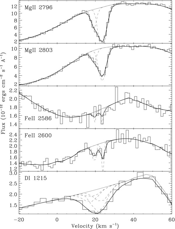
Figure 2. Fits to interstellar absorption lines observed toward HD 35296, plotted on a heliocentric velocity scale. Dashed lines are individual ISM components, and thick solid lines are the sum of all components convolved with the instrumental line profile to fit the data.
Download figure:
Standard image High-resolution imageTable 1. Fit Parametersa
| Ion | λrestb | vc | b | log N |
|---|---|---|---|---|
| (Å) | (km s−1) | (km s−1) | ||
| Mg ii | 2796.3543, 2803.5315 | 19.39 ± 0.42 | 1.75 ± 0.46 |  |
| 23.61 ± 0.12 | 2.15 ± 0.18 | 12.340 ± 0.025 | ||
| Fe ii | 2586.6500, 2600.1729 | 19.55 ± 0.31 | 0.77 ± 0.56 | 11.69 ± 0.10 |
| (23.83 ± 0.31) | 0.63 ± 0.34 |  |
||
| D i | 1215.3430, 1215.3376 | 19.26 ± 0.71 | 5.2 ± 2.0 | 12.44 ± 0.22 |
| (23.47 ± 0.71) | 5.0 ± 1.3 | 12.80 ± 0.14 | ||
| H i | 1215.6682, 1215.6736 | 18.95 ± 0.51 | 11.66 ± 0.23 | 17.329 ± 0.008 |
| (23.17 ± 0.51) | (11.66 ± 0.23) | (17.689 ± 0.008) |
Notes. aQuantities in parentheses are fixed rather than derived (see text for details). bIn vacuum. cCentral velocity in a heliocentric rest frame.
Download table as: ASCIITypeset image
Being so close to the downwind direction, the HD 35296 line of sight is particularly useful for assessing the speed of the local ISM flow. This has recently become an important issue, as an IBEX assessment of the LIC flow vector based on measurements of interstellar helium flowing through the solar system has reduced the inferred LIC speed from the VLIC = 26.3 ± 0.4 km s−1 value derived from older Ulysses helium observations (Witte 2004) to VLIC = 23.2 ± 0.3 km s−1, enough of a decrease to potentially change the ISM flow from supersonic to subsonic (Bzowski et al. 2012; Möbius et al. 2012; McComas et al. 2012a; Zieger et al. 2013). Support for this lower velocity comes from a reassessment of the LIC vector from ISM absorption lines. Using a large compilation of absorption line data, Redfield & Linsky (2008) identified 15 nearby ISM clouds, including the LIC, and estimated the velocity vectors of these clouds. Like the IBEX vector, the LIC vector of Redfield & Linsky (2008) also has a low velocity, VLIC = 23.84 ± 0.90 km s−1, compared with prior estimates from absorption line data that were in better agreement with Ulysses (Lallement & Bertin 1992; Lallement et al. 1995).
Although the new LIC velocities from absorption lines and IBEX appear to be discrepant from Ulysses measurements, the new LIC temperature measurements are not significantly different, with Ulysses, IBEX, and absorption lines suggesting T = 6300 ± 340 K (Witte 2004), T = 6300 ± 390 K (McComas et al. 2012a), and T = 7500 ± 1300 K (Redfield & Linsky 2008), respectively. We compute a LIC temperature and nonthermal velocity for the HD 35296 line of sight using the Doppler parameters measured for Mg ii, Fe ii, and D i (see Table 1), following the procedures of Redfield & Linsky (2004b). The Doppler parameter is related to temperature, T (in K), nonthermal velocity, ξ (in km s−1), and element atomic weight, A, via the equation
Using the χ2 statistic as an indicator of goodness-of-fit (Bevington & Robinson 1992), we find which T and ξ values best fit the LIC Mg ii, Fe ii, and D i Doppler parameters by determining which T and ξ minimize χ2. Uncertainties (1σ) in T and ξ are computed by fixing each parameter in turn and calculating the Δχ value appropriate for the 68.27% confidence level, as described by Bevington & Robinson (1992). The result is  K and ξ < 1.7 km s−1. The large uncertainties are mostly due to uncertainties introduced by the presence of the highly blended second component, which can be hard to quantify. These measurements are consistent with the average LIC properties of T = 7500 ± 1300 K and ξ = 1.62 ± 0.75 km s−1 (Redfield & Linsky 2008).
The HD 35296 line of sight is only 3° from the downwind direction according to both the IBEX and new absorption line LIC vectors. A precise calculation of the projected LIC velocity toward the near-downwind line of sight to HD 35296 yields the following velocity predictions from the Ulysses, IBEX, and absorption line vectors: 26.1, 23.2, and 23.8 km s−1, respectively. The latter two are in excellent agreement with the location of the strongest absorption component observed toward HD 35296, which is at 23.61 ± 0.12 km s−1 for Mg ii. Thus, our HD 35296 data also appear to support the new lower VLIC = 23–24 km s−1 velocity. Incidentally, the weaker absorption component seen toward HD 35296 is not associated with any of the clouds identified by Redfield & Linsky (2008). This is not that unusual, as almost 20% of observed absorption components in the Redfield & Linsky (2008) data set are currently unidentified with a particular cloud.
3. HELIOTAIL ABSORPTION TOWARD HD 35296
The H i Lyα line observed from HD 35296 is displayed in Figure 3. The stellar emission line is greatly affected by broad absorption from interstellar H i centered at 1215.8 Å and much weaker D i absorption at 1215.4 Å. The geocoronal Lyα emission feature mentioned in Section 2 lies in the saturated core of the broad Lyα absorption, but it has been removed in Figure 3. The broad width of the Lyα absorption makes analysis of this line more complex than the analysis of the narrow ISM lines in Figure 2. Our analysis follows procedures used extensively in the past (Wood et al. 2005). The process relies heavily on assumptions of self-consistency between the D i and H i absorption. For H i, all three of the ISM parameters mentioned in Section 2 (v, b, and N) can be tied to D i. We naturally require that  . Since past work has demonstrated that thermal broadening dominates D i and H i absorption lines observed from the local ISM, we can assume
  . And finally, because the gas-phase D/H ratio is known and accepted to be constant in the ISM near the Sun, we can assume
  (Wood et al. 2004).

Figure 3. (a) Lyα line of HD 35296 shown in histogram format on a heliocentric wavelength and velocity scale, with broad H i absorption at 1215.8 Å and narrow D i absorption at 1215.4 Å. The dotted line represents the best fit to the data with only ISM absorption, forcing the D i and H i absorption to be self-consistent. Residuals are shown below the fit. The quality of the fit is poor, especially around D i, and the reconstructed stellar Lyα line (solid line) is clearly blueshifted relative to the stellar rest frame (dot–dashed line). (b) Another fit to the data like (a) but with the addition of a non-ISM absorption component (dashed line), and with a stellar profile (upper solid line) forced to be centered on the stellar rest frame. This fit is also poor. (c) An ISM-only fit to the data using the same stellar profile from (b), but with the fitted region confined to the blue side of the line. The fit is fine, but there is excess H i absorption on the red side of the line (shaded region) that the ISM cannot account for, which is presumed to be from the heliotail.
Download figure:
Standard image High-resolution imageWith these assumptions, it is actually possible to infer the H i fit parameters entirely from those listed for the D i fit in Table 2. However, this is not the same as demonstrating that those H i fit parameters are actually consistent with the observed H i absorption. We therefore fit both D i and H i simultaneously in Figure 3. This fitting process requires the reconstruction of the background stellar Lyα profile. The D i column in Table 2 and the D/H ratio quoted above predict  toward HD 35296. The broad damping wings of the H i absorption depend only on N(H i), so this N(H i) estimate allows us to reconstruct the wings of the stellar profile. We then use the shape of the Mg ii k line to extrapolate in between the two wings, over the saturated core of the H i absorption, the justification being that both H i Lyα and the Mg ii k line are highly opaque chromospheric resonance lines with similar line profiles in solar spectra. An initial fit to the data is performed, and then modifications to the assumed stellar Lyα profile are made to improve the quality of the fit. A couple more iterations of this yields the final result in Figure 3(a). Note that for all our H i Lyα fits we assume that the two ISM components have the same velocity separation and column density ratio for H i as they do in the D i-only fit, and we assume the two ISM components have identical Doppler parameters.
Table 2. Model Input Parameters
| Model 1 | Model 2 | Model 3 | |
|---|---|---|---|
| Solar wind parameters (1 AU) | |||
| n(H+)SW (cm−3) | 6.4 | 7.4 | (see text) |
| VSW (km s−1) | 442 | 432 | (see text) |
| Mach number | 4.2 | 10 | 6.2 (at equator) |
| Consider BSW? | N | N | Y |
| Latitudinal dependence? | N | N | Y |
| ISM parameters | |||
| n(H°)ISM (cm−3) | 0.18 | 0.18 | 0.14 |
| n(H+)ISM (cm−3) | 0.06 | 0.06 | 0.04 |
| VISM (km s−1) | 26.4 | 26.4 | 26.4 |
| TISM (K) | 6530 | 6530 | 6530 |
| BISM (μG) | 3.5 | 4.4 | 4.4 |
| α (deg) | 45 | 20 | 20 |
| Tail extent (AU) | 10000 | 6000 | 6000 |
Download table as: ASCIITypeset image
The fit in Figure 3(a) is not very good, especially near D i. The fundamental problem is that the H i absorption is redshifted relative to D i, making it impossible to fit H i and D i in a self-consistent manner. The narrow D i absorption is being forced to be too broad and too redshifted to fit the actual D i absorption feature. Another problem becomes apparent if the reconstructed stellar Lyα line profile is compared with the stellar radial velocity of 37.8 km s−1 (Nordström et al. 2004). The line profile is clearly blueshifted relative to this velocity (see Figure 3(a)). This can be explained by the presence of very broad heliotail absorption in the red wing of the line, which is not being accounted for in the Figure 3(a) fit. It is exactly this kind of induced line blueshift that led to the identification of heliotail absorption for the three lines of sight discussed in Section 1 (Wood et al. 2007b). The existence of the induced blueshifts near the downwind direction and their absence away from it are what make the heliotail absorption detections particularly convincing. Quantitatively, the stellar Lyα profile used in the fit in Figure 3(a) is shifted by Δv = −4.0 km s−1 relative to the stellar rest frame. This can be compared to the Δv = −5.8 km s−1 shift found for χ1 Ori (Wood et al. 2007b).
In the past, we have sometimes used an absorption component to represent heliospheric absorption (e.g., Wood et al. 2005). However, in this instance, if the stellar profile is forced to be centered on the stellar rest frame, we find a single heliospheric component cannot help to fit the red side of the line very well. This is shown in Figure 3(b). The heliospheric absorption component (dashed line) has the following fit parameters: v = 44.5 km s−1, b = 44.2 km s−1 (corresponding to T = 120, 000 K), and log NH = 13.96. The fit is poor, especially at wavelengths above 1216.2 Å (corresponding to velocities above 130 km s−1), but even if it was a good fit, the fit parameters should still not be taken too seriously, since the absorption is really an integration over a long heliospheric line of sight, with the hydrogen properties varying along that line of sight.
In Figure 3(c), we redo the H i+D i fit, this time focusing only on the blue side of the line, using a stellar Lyα profile forced to be centered on the stellar radial velocity. This leads to a good fit to the data, and the H i parameters for this fit are listed in Table 1. As illustrated in Figure 3(c), there is absorption on the red side of the line that cannot be accounted for by the ISM. It is this absorption that we propose is from the heliotail.
The LIC H i Doppler parameter from the fit quoted in Table 1 corresponds to a temperature of T = 8200 ± 400 K, significantly higher than what the LIC b(D i) value from the D i-only fit would suggest, but still within the broad errors in the LIC temperature formally computed in Section 2. Note that the small uncertainty in the LIC b(H i) value should not be taken seriously, as it is largely a result of the assumptions in the H i fit described above, namely the forcing of the two ISM components to have the same b(H i) and a column density ratio consistent with that of the D i fit. Inconsistencies between the D i-only fit and the D i+H i fit are indicative of the differences in the fit assumptions and the very different estimations of background flux over the absorption features. These would be systematic uncertainties not quantified by the random errors quoted in Table 1.
The characteristics of the heliotail absorption toward HD 35296 are similar to the absorption detected for the other three downwind lines of sight. The data for two of these detections, HD 28205 and HD 28568, suffer from low signal-to-noise, so the χ1 Ori example represents by far the clearest previous detection of the heliotail absorption (Wood et al. 2007b). In Figure 4, the χ1 Ori and HD 35296 absorption are directly compared. A meaningful comparison is only possible away from the saturated core of the Lyα absorption, which limits the relevant velocities to v > 65 km s−1. The HD 35296 absorption appears to be deeper at v < 100 km s−1 than that of χ1 Ori, and it decreases smoothly until it disappears at about v = 275 km s−1. The χ1 Ori absorption seems more structured, with distinct minima near v = 140 km s−1 and v = 265 km s−1. It is not clear whether this structure is indicative of real velocity structure in the heliotail toward χ1 Ori, or if this is just an artifact of uncertainties in the exact shape of the background stellar Lyα profile, which is being inferred by reflecting the blue wing of the line onto the red wing.

Figure 4. Comparison of the heliotail absorption toward HD 35296 (thick green line) and χ1 Ori (thin red line), plotted on a heliocentric velocity and wavelength scale. The normalized flux values are relative to the line-of-sight Lyα absorption after ISM absorption is included (e.g., the dotted line in Figure 3(c)).
Download figure:
Standard image High-resolution image4. MODELING THE HELIOTAIL
4.1. Model Description
We can further explore the issue of heliotail properties using sophisticated numerical models, and we can try to use these models to reproduce the observed heliotail absorption. The models we use here trace their origins to those of Baranov & Malama (1993, 1995), which were the first global heliospheric models with a full kinetic treatment of neutrals. The neutrals are computed self-consistently with the plasma, which is treated as a single hydrodynamic fluid. The detailed treatment of neutrals is particularly important for confronting the HST Lyα data, since the Lyα absorption is coming from heliospheric neutral hydrogen that is wildly out of thermal and ionization equilibrium with the heliospheric plasma.
The original two-dimensional (2D) axisymmetric hydrodynamic code has been expanded into a fully 3D MHD treatment (Izmodenov et al. 2005; Wood et al. 2007a), which can take into consideration the effects of BISM, as well as the magnetic field carried away from the Sun by the solar wind. Using this code, we here present three different models of the heliosphere in order to explore how heliotail shape might be affected by various input parameters and assumptions. These models are the first 3D MHD models of the heliosphere with both extended tails and a kinetic treatment of neutrals. Both of these features are essential for accurately computing Lyα absorption downwind. Past work has indicated that significant Lyα absorption can come from as far away as 3000 AU (Wood et al. 2009). Thus, to ensure that a model accounts for all absorption downwind, a model must extend at least 3000 AU downwind. Extending the model grid this far carries a computational cost, especially for a 3D MHD model. Past extended tail models have been 2D axisymmetric models (Izmodenov & Alexashov 2003; Alexashov et al. 2004),
Table 2 lists the input parameters for the three models. These include the inner solar wind boundary conditions at 1 AU, specifically the proton density [n(H+)SW], wind velocity [VSW], and Mach number. While Models 1 and 2 assume a spherically symmetric solar wind with no magnetic field (BSW), Model 3 provides more complex solar wind boundary conditions, which are described in more detail below. The outer ISM boundary conditions listed in Table 2 include the proton density [n(H+)ISM], neutral hydrogen density [n(H°)ISM], velocity [VISM], temperature [TISM], magnetic field [BISM], and magnetic field orientation [α]. The field orientation, α, indicates the assumed angle between the upwind direction of the ISM flow vector and the ISM field direction, assuming the field lies within the HDP (see Section 1; Lallement et al. 2005, 2010). As noted in the last line of Table 2, all three models have grids that extend at least 6000 AU downwind, in order to include enough of the heliotail to capture all of the heliospheric Lyα absorption in that direction.
The models listed in Table 2 assume a fast ISM flow speed more consistent with the older ISM vector from Ulysses (Witte 2004) than the somewhat slower vectors more recently measured from ISM absorption lines (Redfield & Linsky 2008) and from IBEX data (Bzowski et al. 2012; Möbius et al. 2012). However, the modest differences between these ISM vectors are not large enough to affect our conclusions here. To verify this, we experimented with a version of Model 3 with the slower IBEX VISM value. As expected, this had minimal effect on the predicted Lyα absorption downwind. Furthermore, even though the lower VISM value results in a heliosphere without a bow shock (McComas et al. 2012a), the absorption upwind does not change much either, consistent with the recent findings of Zank et al. (2013).
In the models, the z-axis is defined by the ISM flow direction, with the positive direction being upwind from the Sun. Figure 5 shows slices through the models perpendicular to the z-axis at distances of z = −500 AU on the left and z = −2000 AU on the right. For the former, the color scale indicates the sum of thermal and magnetic pressure, and the arrows show magnetic field lines projected onto the image plane. For the latter, the color scale shows the density of population 2 neutral H. Figure 5 shows how the interstellar field is diverted around the region of space containing the post-TS solar wind flow, which has been diverted into the heliotail. The heliotail is compressed in the direction perpendicular to the ISM field direction. Models 1 and 2 both assume a spherically symmetric solar wind with no magnetic field. For Model 1, the heliotail is still relatively symmetric about the ISM flow axis, but for Model 2 the heliotail is clearly deflected to the right. Both the higher BISM and lower α play a role in creating this deflection (Izmodenov et al. 2009).
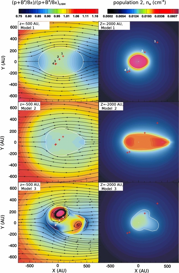
Figure 5. Heliotail structure suggested by Models 1–3 (see Table 2). The left panels show the sum of thermal and magnetic pressure for planes perpendicular to the ISM flow axis at z = −500 AU from the Sun. The right panels show the population 2 neutral density at z = −2000 AU from the Sun. Arrows in the left panels are the magnetic field lines projected onto the plane. The outline of the heliopause is in white, indicating the shape of the heliotail. Small plus signs indicate the positions of stars with detected heliotail Lyα absorption, where the numbered stars are: (1) χ1 Ori, (2) HD 35296, (3) HD 28568, and (4) HD 28205.
Download figure:
Standard image High-resolution imageModel 3 is identical to Model 2 except for a much more sophisticated treatment of the solar wind. Within the ecliptic, time-averaged measurements from spacecraft at 1 AU are used for input parameters, including measurements of the magnetic field. Latitudinal variation of solar wind properties is also assumed, where the latitudinal dependence is estimated from measurements by SOHO/SWAN, Ulysses, and radio scintillation data (Lallement et al. 2010; Sokół et al. 2013). The assumed latitudinal dependence is characteristic of a solar minimum wind, with high speed streams emanating from the solar poles, and slow speed wind coming from lower latitudes. The initially bipolar high speed wind streams are deflected into the tail to form the bipolar heliotail in Figure 5. The more complex solar wind leads to a heliotail significantly more asymmetric and irregular in shape than for Models 1 and 2 with spherically symmetric winds.
4.2. Heliotail Deflection and Asymmetry
The locations of the four stars with detected heliotail absorption are indicated in both Figures 1 and 5. At z = −2000 AU, χ1 Ori is outside the heliotail in all three models, while HD 35296 is inside or just outside, a situation perhaps consistent with there being somewhat less heliotail absorption observed toward χ1 Ori than toward HD 35296, at least at v < 100 km s−1 (see Figure 4). In principle, it should be possible to explore heliotail asymmetry and deflection using the heliotail Lyα absorption diagnostic, but four lines of sight are clearly not enough to do this in any great detail. The right panels of Figure 5 demonstrate that population 2 neutrals exist outside the heliotail, due to the propensity of neutrals to effortlessly cross field lines, and boundaries such as the HP. This and line-of-sight integration effects mean that absorption asymmetries will not be as well defined as Figure 5 might suggest. Nevertheless, the existing Lyα data still place limits on possible heliotail asymmetry and deflection.
Figure 1 illustrates that there are HST Lyα observations within IBEX's dark ENA spot (e.g., τ Cet,  Eri) that do not show any heliotail absorption, contradicting the notion of an offset heliotail pointing in that direction. In order to explore why absorption from population 2 neutrals is observed downwind, and not toward the stars within the dark ENA spot, in Figure 6 we plot traces of density, temperature, and radial velocity toward HD 35296 and τ Ceti, using Model 3 as an example. These traces are shown for both protons (dashed lines) and population 2 neutrals (solid lines). The temperatures and velocities are computed by taking moments of the velocity distributions, but for the population 2 neutrals it is important to keep in mind that these distributions are not Maxwellian.

Figure 6. Traces of density, temperature, and radial velocity for protons and population 2 neutral hydrogen; for both the very downwind line of sight to HD 35296 and the more sidewind line of sight toward τ Ceti.
Download figure:
Standard image High-resolution imageToward τ Ceti, the TS and HP are encountered at 106 AU and 190 AU, respectively, marked clearly by sharp changes in plasma density, temperature, and velocity. Toward HD 35296, there is a clear TS crossing at 118 AU, but the HP in this very downwind direction is much fuzzier, apparently lying somewhat beyond 1000 AU. Inspection of the population 2 density curves in Figure 6 reveals why absorption from these neutrals is more detectable toward HD 35296 than toward τ Ceti. In both directions, the population 2 density increases beyond the TS all the way to the HP, before decreasing quickly beyond that. However, toward τ Ceti the density never rises above 0.0011 cm−3 since the HP is so close to the TS, while toward HD 35296 the density reaches 0.0069 cm−3. Even more telling is the line-of-sight integrated column density, which toward τ Ceti is only log NH = 12.83, compared with log NH = 14.24 toward HD 35296, a factor of 25 difference. Note that this log NH = 14.24 prediction of Model 3 is in decent agreement with the crude empirical estimate of log NH = 13.96 from the Figure 3(b) fit described in Section 3, despite our reservations about the reliability of that estimate.
The clustering of the heliotail detections about the downwind direction in Figure 1 strongly implies a heliotail centered close to that location. It surely rules out large heliotail deflections of >20°. Although Models 2 and 3 do show significant deflection of the heliotail away from the downwind direction, the amount of deflection is <10°, consistent with the locations of heliotail Lyα absorption detections only close to the downwind direction. This very modest degree of heliotail deflection is consistent with previously published 3D MHD models (Pogorelov et al. 2008).
To summarize, we conclude that although BISM may strongly affect the shape and orientation of the TS and HP in the upwind and sidewind directions, as suggested by the Voyager and IBEX observations mentioned in Section 1, the models and Lyα observations presented here strongly suggest that downwind from the TS the ISM flow pressure reasserts itself and largely controls the direction of the distant heliotail. This is in large part due to the effects of charge exchange with ISM neutrals, which are not affected by magnetic fields. Quantitatively, the clustering of the heliotail detections about the downwind direction rules out large heliotail deflections of >20°.
4.3. Absorption Predictions
We can test the models listed in Table 2 by comparing the Lyα absorption that they predict to observed heliospheric absorption. We have done this before for various other models derived from the Baranov & Malama (1993, 1995) heritage (Izmodenov et al. 2002; Wood et al. 2007a, 2007b, 2009). The data/model comparison for Models 1–3 is shown in Figure 7. Many lines of sight are available for these purposes (see, e.g., Wood et al. 2007a), but only four are shown here. The figure focuses on the red side of the Lyα absorption profile where the heliospheric absorption resides, plotted on a heliocentric velocity scale.

Figure 7. Comparison of the heliospheric Lyα absorption predicted by Models 1-3 with actual absorption observed by HST for four lines of sight. The focus is on the red side of the Lyα absorption profile. As in Figure 4, the normalized flux values are relative to the line-of-sight Lyα absorption after ISM absorption is included. The ecliptic coordinates (λe, βe) and angular distance from the upwind direction of the ISM flow (θ) are indicated for each line of sight. The heliospheric absorption for the two upwind lines of sight (36 Oph, α Cen) is mostly from population 3 neutrals, while that for the two downwind lines of sight (χ1 Ori, HD 35296) is predominantly from population 2 neutrals. Note the much larger velocity scale for the downwind lines of sight to encompass the broader absorption.
Download figure:
Standard image High-resolution imageWe are naturally interested here mostly in absorption observed toward the heliotail, so the figure shows the χ1 Ori and HD 35296 data. However, we also show two upwind lines of sight with detected heliospheric absorption, 36 Oph and α Cen, to demonstrate that Models 1-3 are reasonably successful in reproducing the absorption observed upwind. We note once again that in upwind directions the heliospheric absorption is dominated by population 3 neutrals created in the hydrogen wall, as opposed to the post-TS neutralized solar wind (i.e., population 2) responsible for most of the absorption downwind.
Focusing on the downwind directions, in all the models the population 2 neutral opacity increases toward lower velocities, being at a maximum near the ∼25 km s−1 speed of the undisturbed ISM flow. This low velocity might be surprising at first, given that the velocity of the post-TS solar wind plasma is >100 km s−1 (Richardson et al. 2009), but Figure 6 shows that in the heliotail the plasma velocity decreases toward the ISM speed even before the HP is reached, and the speed of population 2 neutrals not surprisingly trends toward that velocity as well. An important factor here is that charge exchange probabilities are higher with protons moving at velocities more similar to the ∼25 km s−1 speed of the ISM neutrals that have made it into the heliotail, so much of the charge exchange involves protons moving slower than the average post-TS wind flow. A curious feature of the neutral velocity in Figure 6 is that it is actually negative just beyond the TS (and thereby below the lower bound of the figure). This indicates that at that location most of the population 2 neutrals are ones that have been created farther out and are actually moving inward. The high temperature of the post-TS region and corresponding broad distribution of velocity is what allows this to happen.
In the downwind direction the agreement of the models with the data is decent but not quite as good as upwind. All three models overpredict the observed absorption, with predicted Lyα opacities being a factor of 2–3 too large in the 50–150 km s−1 velocity range. Comparing the absorption predicted by Models 2 and 3 provides an indication of how sensitive the downwind absorption is to the solar wind boundary conditions, given that these two models are identical except for these boundary conditions. The difference in predicted absorption of the two models in Figure 7 is insignificant upwind but quite large downwind, indicating that the issue of how to treat the complicated wind of the real Sun in global heliospheric models of this nature is a significant source of uncertainty for downwind absorption predictions. These uncertainties could then be a significant contributor to the models' factor of 2–3 overprediction of Lyα opacity downwind.
In assessing how well the models reproduce the observed heliotail absorption, it should be noted that Models 1–3 all suffer from an insufficiently sophisticated treatment of the plasma, which past work has demonstrated can affect absorption predictions downwind (Wood et al. 2007b). The standard approach, used in Models 1–3, is to treat the heliospheric plasma as a single fluid everywhere, but this is observationally known to be simplistic. For example, pickup ions inside the TS do not thermalize with the bulk solar wind plasma. Thus, describing the plasma inside the TS with a single Maxwellian fluid naturally leads to inaccuracies in the plasma velocity distributions, inaccuracies that are carried beyond the TS into the inner heliosheath.
Malama et al. (2006) have attempted to solve this problem by developing a complex multi-component treatment of the plasma. As yet, it is too computationally expensive to apply this approach to a 3D MHD model. However, experience with 2D axisymmetric models indicates that while the multi-component treatment has little effect on hydrogen wall absorption upwind, it does lead to significant reduction in the heliotail absorption downwind (Wood et al. 2007b). This provides another possible explanation for the overprediction of absorption downwind by our models.
We can also use the models to explore asymmetries in absorption that one might expect to see due to heliospheric asymmetries. This is done in Figure 8 for Model 2 and in Figure 9 for Model 3. In each figure there are panels for five different values of θ, where θ is the angle between the line of sight and the upwind direction of the ISM flow. In each panel, absorption is computed for eight different azimuthal angles, ϕ, where ϕ = 0° and ϕ = 180° would be in the plane of the magnetic field. The degree of variation among the eight azimuthal curves indicates the degree of absorption variability associated with heliospheric asymmetry. Similar figures were presented by Wood et al. (2007a, 2012), but we here focus on downwind directions with θ ⩾ 140°. Black lines in each panel show the absorption directly downwind (i.e., at θ = 180°), so Figures 8 and 9 show nicely how absorption increases with increasing θ, indicating once again how absorption from population 2 neutrals becomes more detectable closer to downwind.

Figure 8. Illustration of the directional dependence of Lyα absorption predicted by Model 2 (see Table 2). Absorption profiles are shown for five values of the poloidal angle θ (the angle between the line of sight and the upwind direction of the ISM flow), and eight values of the azimuthal angle ϕ, where the plane of the ISM magnetic field is in the plane containing ϕ = 0° and ϕ = 180°. The focus is on downwind directions with θ ⩾ 140°, and the thick black line in each panel indicates the absorption directly downwind, for comparison.
Download figure:
Standard image High-resolution image
Figure 9. Same as Figure 8, but for Model 3.
Download figure:
Standard image High-resolution imageComparing Figures 8 and 9 demonstrates that the more complex latitudinally variable solar wind assumed in Model 3 leads to a significant increase in absorption variation with ϕ compared with Model 2. In principle, this degree of variability might be detectable if enough HST observations of sufficiently high quality were obtained. However, the existing four lines of sight are certainly not enough to do this.
4.4. Comparison with IBEX Observations of the Heliotail
Although the models and Lyα data do not support the offset heliotail interpretation initially offered to explain the ENA dark spot observed by IBEX, Model 3 does potentially support the revised interpretation offered by McComas et al. (2013). As first mentioned in Section 1, McComas et al. (2013) note the presence of a second, somewhat less prominent dark ENA lobe on the other side of the downwind direction, with both lobes being characterized by high spectral slopes. The two lobes are proposed to be associated with slow wind regions compressed toward the ecliptic plane by the overexpanding high speed wind emanating from the Sun's polar regions. This picture is consistent with the bipolar nature of the heliotail seen in Figure 5 for Model 3, which shows the higher pressure of the polar wind regions, and lower pressure in between the two high pressure lobes, where the ecliptic plane and slow wind would reside.
The reason for the lower ENA fluxes from the slow wind regions is presumably that for slow wind there is less energy in the bulk wind flow to be converted to thermal energy at the TS, leading to a steeper ENA spectrum and low ENA fluxes at high energies. This effect is particularly pronounced in the downwind direction where the TS distance is greatest. This is because pickup ion production gradually slows the solar wind. In the upwind direction explored by Voyager 1 and Voyager 2, the amount of deceleration is only ∼50 km s−1 (Richardson et al. 2008), but there could be an additional 50–100 km s−1 deceleration before the TS is reached downwind.
Model 3 cannot directly test this scenario, as the single fluid plasma approximation utilized in this model does not provide proton velocity distributions sufficiently accurate to make ENA flux predictions for comparison with IBEX data. We have already noted in Section 4.3 the inaccuracies in absorption calculation introduced by treating pickup ions and bulk solar wind as a single fluid. Treating the non-Maxwellian nature of the plasma distribution inside and outside the TS is necessary for a model to predict ENA fluxes at IBEX. In the near future, we hope to compute a new version of Model 3 with a more sophisticated treatment of the plasma, allowing for a more direct confrontation with the IBEX observations of the heliotail.
5. SUMMARY
We have presented an analysis of ISM and heliospheric absorption observed toward HD 35296 by HST. We summarize our results as follows:
- 1.The HD 35296 line of sight is of particular interest for being very near the downwind direction of the ISM flow vector seen by the Sun. We observe two ISM velocity components toward HD 35296 (see Figure 2). The one at 23.61 ± 0.12 km s−1 provides support for the 23–24 km s−1 local ISM speed suggested by both IBEX (McComas et al. 2012a) and a recent reassessment of ISM absorption lines (Redfield & Linsky 2008), in contrast to the higher ∼26 km s−1 speed implied by Ulysses (Witte 2004) and older absorption line analyses (Lallement & Bertin 1992; Lallement et al. 1995). We measure a LIC temperature and nonthermal velocity of
 K and ξ < 1.7 km s−1, respectively, values consistent with average LIC values from Redfield & Linsky (2008) within the broad error bars.
 - 2.We clearly detect heliotail Lyα absorption from heliospheric population 2 neutrals in the HST data, similar to previous detections for three other lines of sight within 20° of the downwind direction (Wood et al. 2007b).
- 3.We present the first 3D MHD global heliospheric models with both kinetic neutrals and extended grids toward the heliotail, features necessary to properly model heliotail Lyα absorption. The models are reasonably successful at reproducing the observed absorption, but they overpredict the Lyα opacity downwind by a factor of 2–3, possibly due to uncertainties in how to treat the time and latitudinal dependence of the solar wind, or due to the simplistic single-fluid treatment of plasma in the models.
- 4.The ISM magnetic field induces asymmetries in the heliosphere, and can deflect the heliotail from the downwind direction, but the clustering of the four heliotail absorption detections close to the downwind direction rules out the possibility of large heliotail deflections of >20°. This is consistent with the very modest deflections of <10° indicated by our models.
- 5.Including latitudinal variations in solar wind properties in the models (i.e., Model 3) does not change the expected heliospheric hydrogen wall absorption upwind at all, but it does affect heliotail absorption downwind. Greater heliotail asymmetry is accompanied by larger absorption asymmetries. These are potentially large enough be detectable, but the number of downwind heliotail absorption detections would have to be much higher than the current number of four.
- 6.Model 3 demonstrates that assuming latitudinal variations in the solar wind boundary conditions yields a bipolar heliotail of a nature potentially consistent with that inferred by McComas et al. (2013) from IBEX data.
Support for program GO-12596 was provided by NASA through an award from the Space Telescope Science Institute, which is operated by the Association of Universities for Research in Astronomy, Inc., under NASA contract NAS 5-26555. E.E. acknowledges support through a NASA undergraduate research fellowship from the Connecticut Space Grant Consortium. V.I. and D.A. are partially supported by Programm 22 of the Russian Academy of Sciences and RFBR grant 13-02-00265. The calculations were performed using the supercomputers of Lomonosov Moscow State University ("Lomonosov" and "Chebyshev").
Footnotes
- *
Based on observations made with the NASA/ESA Hubble Space Telescope, obtained at the Space Telescope Science Institute, which is operated by the Association of Universities for Research in Astronomy, Inc., under NASA contract NAS 5-26555. These observations are associated with program GO-12596.