


ABSTRACT
Propagating coronal mass ejections (CMEs) are often accompanied by burst signatures in radio spectrogram data. We present Nançay Radioheliograph observations of a moving source of broadband radio emission, commonly referred to as a type IV radio burst (type IVM), which occurred in association with a CME on the 14th of August 2010. The event was well observed at extreme ultraviolet (EUV) wavelengths by SDO/AIA and PROBA2/SWAP, and by the STEREO SECCHI and SOHO LASCO white light (WL) coronagraphs. The EUV and WL observations show the type IVM source to be cospatial with the CME core. The observed spectra is well fitted by a power law with a negative slope, which is consistent with optically thin gyrosynchrotron emission. The spectrum shows no turn over at the lowest Nançay frequencies. By comparing simulated gyrosynchrotron spectra with Nançay Radioheliograph observations, and performing a rigorous parameter search we are able to constrain several key parameters of the underlying plasma. Simulated spectra found to fit the data suggest a nonthermal electron distribution with a low energy cutoff of several tens to 100 keV, with a nonthermal electron density in the range 100–102 cm−3, in a magnetic field of a few Gauss. The nonthermal energy content of the source is found to contain 0.001%–0.1% of the sources thermal energy content. Furthermore, the energy loss timescale for this distribution equates to several hours, suggesting that the electrons could be accelerated during the CME initiation or early propagation phase and become trapped in the magnetic structure of the CME core without the need to be replenished.
1. INTRODUCTION
Traditionally, studies of the initiation and propagation phases of coronal mass ejections (CMEs) have used extreme ultraviolet (EUV) images to cover the low corona, and white light (WL) coronagraph images to cover the high corona and interplanetary medium. WL coronagraph observations have revealed that CMEs exhibit a typical three-part structure: a bright core of erupting filamentary material, a dark cavity and a bright leading edge. While WL coronagraphs image the Thomson-scattered photospheric light, Bastian & Gary (1997) found that radio observations at meter wavelengths, such as those from the Nançay Radioheliograph (NRH: Kerdraon & Delouis 1997), are ideal for investigating sources electron acceleration within the CME. For example, sources of coherent plasma emission and incoherent gyrosynchrotron emission can be imaged by NRH and are a well-established diagnostics of electron acceleration (e.g., Bastian & Gary 1997).
CMEs are often associated with a variety of radio bursts observed at metric and decametric wavelengths. In this paper we present radio observations from NRH, of a type IV radio burst, which occurred in association with a CME on the 14th of August 2010. These events were first classified by Boischot & Denisse (1957) as a flare-related source of broadband radio emission moving outward from the Sun. Since their initial classification, a number of stationary sources with similar spectral characteristics were also classified as type IV radio bursts. This lead to the necessity for two subcategories: a moving type IV burst (type IVM) and a stationary type IV burst (type IVS), to distinguish between such events (Weiss 1963). In some cases, the type IVS appears after the moving type IVM burst, and is located above the associated flare site (Wild 1969).
The bursts are found to appear around 1.8 R☉ and propagate out to around 2 to 3 R☉ before fading (Smerd & Dulk (1971) with 80 MHz observations from the Culgoora Radioheliograph and Robinson (1978) with 80 and 160 MHz Culgoora observations), though some bursts have been observed out to 6 R☉ (Riddle 1970). The source brightness temperature is typically less than 5 × 10⁸ K (Robinson 1978) and has a constant, low degree of circular polarization during the early and main phases of the burst. In some cases, this is followed by an increase in polarization to ⩾70% in the declining phase of the burst. However, in other cases the burst maintains low or no circular polarization throughout its duration. In a study by Robinson (1978), several events began as a single source before splitting into sometimes multiple secondary sources. In some events these multiple sources were bipolar, while others had an unpolarized central source with oppositely polarized secondary and tertiary accompanying sources on either side (Wild 1969). The latter has been attributed to an expanding magnetic arch with the radio sources being related to the apex and legs of the loop respectively. With knowledge of the polarization and the magnetic field direction, the intrinsic mode of the emitted radiation, extraordinary (x) or ordinary (o), can be determined. This diagnostic can be used to determine the emission mechanism, e.g., gyrosynchrotron emission is o-mode in the optically thin regime and x-mode at optically thick frequencies (Ramaty 1969). Fundamental plasma emission could potentially show o-mode polarization, since the x-mode absorption coefficient is always greater, while plasma emission at its harmonic is not expected to be polarized. Polarization measurements can also be a diagnostic of the viewing angle, θ, of the observer with respect to the magnetic field direction. For the case of gyrosynchrotron emission, the polarization can be large for small values of θ, and decrease as θ increases. Furthermore, polarization observations will also show signatures of particle anisotropies (Fleishman & Melnikov 2003).
So far, there has not been a general consensus regarding the mechanism which produces the observed emission in type IV radio bursts. Boischot & Denisse (1957) first postulated the burst resulted from synchrotron emission on the basis that, firstly, the type IV source positions were observed at heights greater than the expected plasma level of the observing frequency. Thus requiring the local electron density to be considerably higher than that predicted by coronal density models, i.e., enhanced by a factor 40 at 3 R☉ and a factor 100 at 6 R☉ (Duncan 1981). However EUV observations have found the electron density in propagating plasmoids can be of the order 109 cm−3 (Hannah & Kontar 2013), which is sufficient for Langmuir wave production at such heights. Secondly, initial 1D interferometric observations showed no spatial dispersion of the source position across several frequencies, as would be expected if the emission was caused by plasma radiation, though this was disregarded when 2D observations found spatial dispersion within some type IV events (McLean 1973; Nelson 1977). Synchrotron theories face problems when trying to explain the brightness and high degree of polarization often observed. It is not expected that synchrotron emission will be highly polarized when the viewing angle between the observer and the magnetic field is large, as is likely the case for type IV sources which are preferentially observed for limb events. For polarization of ⩾70%, the viewing angle with respect to the magnetic field should be no more than ±30° (Duncan 1981). To produce such high polarization requires straight, poloidal magnetic field within the source. It is difficult to envisage how this would occur for an erupting plasmoid, and how this would result in the fragmentation of the source into multiple sources (Robinson 1978). For synchrotron emission to produce the evolving characteristics of the burst, specific conditions regarding the optical depth of the x and o-modes, and the magnetic field structure within the burst must be satisfied (Robinson 1974; Gary et al. 1985). Alternatively, several papers have suggested that plasma emission could account for the observed emission and in particular, could favor high polarization and the observed o-mode polarization (Duncan 1981).
The velocity at which the source propagates away from the Sun has been seen to fall loosely into two groups (Robinson 1978): slow moving bursts with a velocity of around 200 km s−1; and faster moving bursts with velocities of around 1500 km s−1. It is thought that the fast moving bursts are produced in association with a shock (Smerd & Dulk 1971; Robinson 1978) while the slower moving bursts are produced by flare accelerated electrons that are confined in an erupting plasmoid. In a small number of events, radio imaging at metric wavelengths has revealed the presence of synchrotron emission from a loop, similar in morphology to the leading edge seen in WL observations, but smaller in extent (Bastian et al. 2001; Maia et al. 2007; Démoulin et al. 2012). Such features are referred to as the radio CME. The optically thin synchrotron emission is thought to be produced by 0.5–5 MeV electrons contained within the CME's magnetic field structure, with a field strength of 0.1 to a few Gauss. In revisiting the events presented in Bastian et al. (2001) and Maia et al. (2007), Démoulin et al. (2012) finds the radio loop to be co-spatial with the CME flux rope cavity. The authors suggest that the synchrotron emitting electrons found in the radio CME are accelerated in a reconnection event occurring below the flux rope. The upward directed accelerated electrons are injected into the flux rope, as expected in the standard model of an eruptive event (Forbes et al. 2006).
In addition to synchrotron emission, a number of hard X-ray observations have revealed the presence of accelerated electrons in association with erupting plasmoids (Hudson 1978; Hudson et al. 2001; Krucker et al. 2007; Glesener et al. 2013). Due to the limited dynamic range of X-ray imagers, it is difficult to observe faint emission in the high corona, particularly in the presence of bright soft X-ray flare loops or hard X-ray footpoints; Each of the aforementioned observations were obtained for events that were highly occulted (up to 0.3 R☉, i.e., for a flare located 40° behind the limb). The X-ray sources were located high above the associated flare loops and were found to contain roughly 0.1%–1% of the total flare energy content. For the event detailed in Krucker et al. (2007), radio observations at 17 GHz and 34 GHz from the Nobeyama Radioheliograph confirmed the presence of accelerated electrons, while in the 3rd of November flare presented in Glesener et al. (2013), radio spectrogram data suggests synchrotron emission at GHz frequencies, (I. Zimovets 2012, private communication).
Although type IV bursts are fairly common at metric wavelengths, the most recent observational studies date back to the 1980s and to instruments which observed the burst simultaneously in only a few passbands. Using NRH observations at ten frequencies between 150 MHz and 445 MHz, in conjunction with cutting edge EUV observations from the Atmospheric Imaging Assembly (AIA: Lemen et al. 2012) onboard the Solar Dynamics observatory (SDO) and the Sun Watcher using Active Pixel System Detector and Image Processing (SWAP: Seaton et al. 2013) telescope onboard the European Space Agency PRoject for OnBoard Autonomy 2 (PROBA2), we revisit the topic with the intent of characterizing the role of type IV bursts within the CME system. In particular, using the increased spectral coverage to investigate which emission mechanism produces the observed radiation and estimate the nonthermal energy content of the source. In Section 2 we present an overview of the evolution of the CME in EUV and WL observations. In Section 3 we give an overview of the radio observations from NRH and in Section 4 we discuss our determination of a number of physical parameters of the emitting plasma.
2. OBSERVATIONAL OVERVIEW
The CME occurred on the 14th of August 2010 and was associated with a GOES C4 class flare produced by NOAA AR 1093, located at N12W56. The flare began around 09:30 UT and peaked in soft X-rays at 10:05 UT. Lightcurves and spectrogram data covering the duration of the event at X-ray and radio wavelengths are shown in Figure 1. From top to bottom, Figure 1 shows the GOES lightcurves (1.6 keV, 3.1 keV), an X-ray spectrogram from the Ramaty High Energy Solar Spectroscopic Imager (RHESSI; 3–230 keV; Lin et al. 2002), radio spectrogram data from Phoenix-3 (250 MHz–850 MHz and 1 GHz–4 GHz) in Bleien, the San Vito radio observatory, part of the USAF Radio Solar Telescope Network (RSTN/San Vito: 70–180 MHz), the Nançay Decameter Array (DAM: 20–70 MHz) and the WAVES instrument onboard the Solar TErrestrial RElations Observatory (STEREO-A/WAVES: 200 kHz–16 MHz). Due to RHESSI spacecraft night and the south atlantic anomaly (SAA), there was no X-ray data available between 09:55 UT and 10:58 UT. The two short gaps prior to this are as a result of the spacecrafts attenuator motions as the count rate increased. Furthermore, radio data from Phoenix-3 in the 1 to 4 GHz range was only available between 09:38 UT and 10:44 UT and between 09:45 UT and 10:45 UT for DAM. The spectrogram data have been processed to remove bad frequency channels which contained noise. Although a number of noisy channels still remain, we have refrained from over cleaning the data such that real data is not removed. A number of radio bursts are observed in the spectrogram data. A type III radio burst is observed between 40 MHz and 250 kHz (DAM and STEREO-A/WAVES) from 09:50 UT until 11:00 UT, indicating that electrons, most likely accelerated during the restructuring of the coronal magnetic field during the CME initiation and lift-off, have access to open field lines. A type II radio burst is observed between 60 MHz and 20 MHz (DAM) from ∼09:52 UT until 10:12 UT, indicating the presence of a shock wave driven either by the propagating CME or formed as the result of a sudden release of energy associated with the accompanying flare. At higher frequencies, in the GHz range, DCIM (Phoenix-3) bursts are observed between ∼09:40 UT and 10:41 UT. We note that the observing frequency range of the Nançay Radioheliograph is from 150 MHz to 445 MHz, corresponding to data observed by RSTN and the lowest frequency Phoenix-3 telescope shown in Figure 1. Due to a strong type I noise storm observed across the entire NRH frequency range (see Figure 3), the signature of the type IV radio burst cannot be isolated in the spectrogram data.

Figure 1. From top to bottom: GOES (1.6 keV, 3.1 keV), RHESSI (3–230 keV), Phoenix-3 (250–850 MHz and 1–4 GHz), USAF Radio Solar Telescope Network (RSTN/San Vito: 70–180 MHz), Nançay Decameter Array (DAM: 20–70 MHz) and STEREO-A/WAVES (200 kHz–16 MHz).
Download figure:
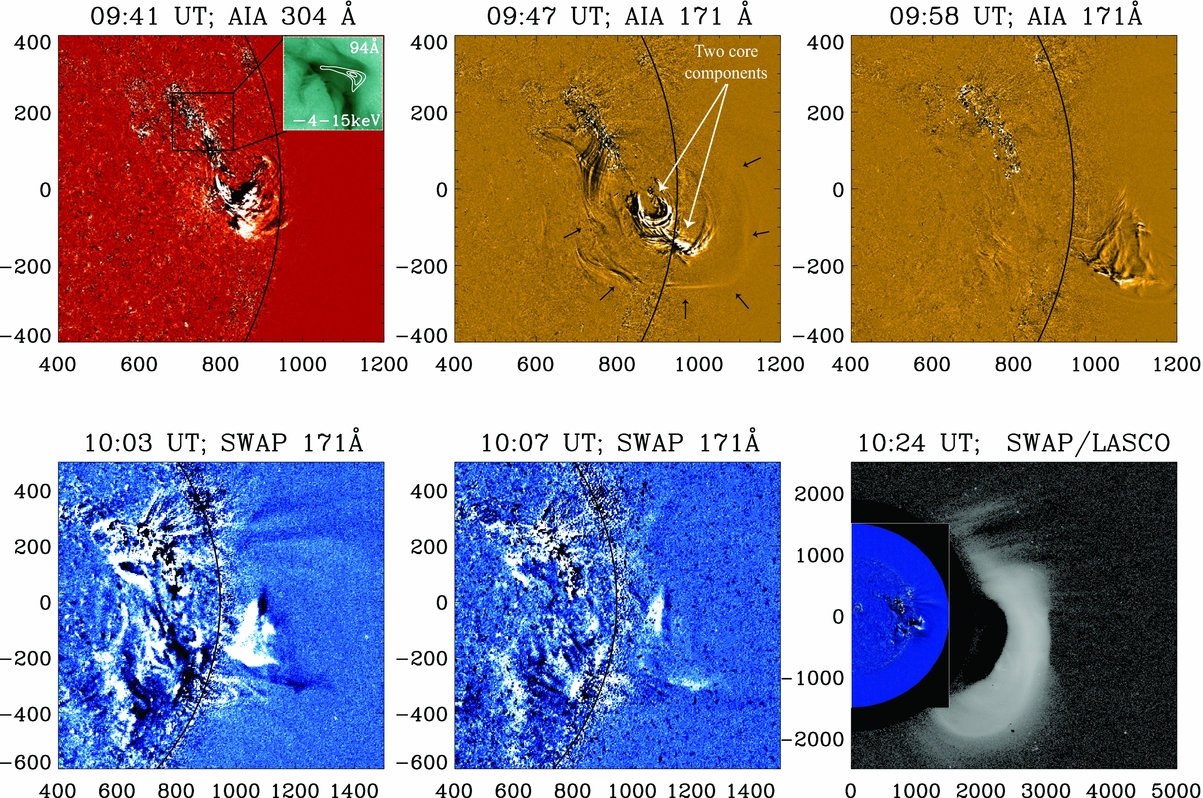
Standard image High-resolution imageFigure 2 shows the temporal evolution of the CME, from its initiation out to 3–4 R☉. The top left panel shows a 304 Å EUV difference image at 09:41 UT from AIA. At this time we can see the erupting filament material that forms the core of the CME (875'', −50'') as it propagates away from the flare site. The inset shows a close up of the flare site (outlined by a square on the main image) with RHESSI X-ray (4–15 keV) image contours overplotted. Observations from RHESSI show only a modest increase above the background at >25 keV. The top middle and right panels of Figure 2 shows AIA 171 Å difference images at 09:47 UT and 09:58 UT. From the image at 09:47 UT, it appears that the CME core has two components (white arrows) which separate and continue to propagate one ahead of the other, with the outer component propagating faster. A faint outer envelope, which possibly forms the leading edge of the CME, is also visible (black arrows). While images from AIA have finer spatial resolution (1''.2), the larger field of view (FOV) of SWAP (41' versus 54', i.e., out to 1230'' and 1620'' respectively) allows us to follow the CME beyond the AIA FOV. The bottom left and middle panels of Figure 2 show SWAP 171 Å difference images at 10:03 UT and 10:07 UT. The bottom right panel of Figure 2 shows a difference image at 10:24 UT from the LASCO C2 coronagraph onboard SOHO, with a 171 Å image from SWAP showing the solar disk. By this time the front of the CME and part of the cavity are visible in the WL chronograph image.

Figure 2. Top left: the left panel shows an AIA 304 Å difference image (red) taken at 09:41 UT. The inset contains a close up of the flare site (indicated by the square) with RHESSI 4–15 keV X-ray image contours overplotted. Top middle and right: AIA 171 Å difference images (yellow) taken at 09:47 UT and 09:58 UT. White and black arrows indicate the two core components and outer envelope, respectively. Bottom left and middle: SWAP 171 Å difference images showing the CME in a wider FOV at 10:03 UT and 10:07 UT. Bottom right: a LASCO C2 difference image at 10:24 UT with a SWAP 171 Å difference image inset showing the solar disk.
Download figure:
Standard image High-resolution image3. RADIO OBSERVATIONS
3.1. Image Preparation
Radio images for this event are available from NRH. Throughout the event, there is a type I noise storm (NS) present that is observed at all NRH observing frequencies. The left panel of Figure 3 shows a pre flare image from AIA 304 Å at 09:20 UT, highlighting the AR and filament material prior to eruption. Radio contours are overplotted for 173 MHz, 228 MHz, 270 MHz, 298 MHz, 327 MHz and 360 MHz, outlining the NS. Contours are shown for 50%, 70% and 90% of the maximum Tb in the full radio map for 173 MHz to 327 MHz, and at 70% and 90% for 360 MHz. Noise storms are typically located in the corona above active regions and are commonly observed below ∼400 MHz. They exhibit two components: slowly varying, broadband emission that can last for several tens of minutes to several days and; numerous short duration, narrowband bursts lasting <1 s, which are superimposed on the slowly varying component. Type I noise storms are evidence for small-scale energy release and electron acceleration events and are often observed prior to a solar flare.

Figure 3. Left: preflare AIA 304 Å image at 09:20 UT with NRH 10 s brightness temperature image contours overplotted for 173 MHz (red), 228 MHz (orange), 270 MHz (dark green), 298 MHz (light green), 327 MHz (blue) and 360 MHz (dark blue). Contour levels are at 50%, 70% and 90% of the maximum Tb of the full radio map. For 360 MHz only 70% and 90% contours are shown. Right: a SWAP 171 Å image at 10:04 UT with NRH 298 MHz 10 s Tb image contours overplotted (white) for 4%, 8%, 16%, 32%, 64% and 96% of the maximum Tb in the full radio map. Green contours show the resulting isolated radio source at 298 MHz after the noise storm contribution is subtracted out. Green contours correspond to 50%, 70% and 90% of the maximum Tb of the CME-RS alone.
Download figure:
Standard image High-resolution imageThe right panel of Figure 3 utilizes the extended field of view of a SWAP 171 Å image to show the erupting plasmoid that becomes the CME core at 10:04 UT, when it is beyond the field of view of AIA. NRH 298 MHz Tb contours (white) are overplotted from a "standard" 10 s NRH map at 4%, 8%, 16%, 32%, 64% and 96% of the maximum Tb. While the NS storm is the dominant source throughout the event, an additional source associated with the CME can be seen propagating away from the sun in a south-west direction. In order to isolate this CME radio source (CME-RS) the radio images were first integrated over 30 s time intervals to improve the signal to noise ratio of the CME-RS. This was achieved by integrating three standard 10 s NRH back projected images and then applying the CLEAN algorithm using beam parameters for the middle time interval. The NS was then fitted with a 2D Gaussian and the contribution removed from the NRH images. It is important to note that the CME-RS feature is already clearly observed in the standard 10 s NRH radio maps, as is shown in the right plot of Figure 3 (NRH images shown in the rest of the paper are made using the 30 s time integrated images). Green contours in Figure 3 (right) show an example of the resulting isolated CME-RS source at 298 MHz, after the NS contribution was subtracted. The plotted contours are for 50%, 70% and 90% of the maximum Tb of the CME-RS alone. This process was carried out for all images at each of the NRH observation frequencies. Since the beam parameters and hence the spatial resolution varies with frequency (292'' FWHM at 150 MHz to 122'' at 360 MHz) the height at which we can isolate the CME source from the NS varies for each frequency. This corresponds to times from around 09:58 UT onward, when it was possible to recover the CME source at all frequencies. The radio analysis presented in the following sections occurs for time intervals after those in the top left and middle panels shown in Figure 2.
3.2. Radio CME Evolution
Figure 4 shows the temporal evolution of the CME-RS with respect to its EUV and WL counterparts, within the AIA, SWAP and LASCO fields of view, respectively. For all panels, NRH radio Tb contours for the isolated CME-RS are plotted at 50%, 70% and 90% of the maximum Tb. For clarity, Figures 2 and 4 use matching image times (to within the EUV/WL image cadence while highlighting changes observed by NRH) for cross-checking sources where NRH image contours may obscure details in the EUV/WL images. The top row of Figure 4 shows AIA 171 Å (left) and SWAP 171 Å (middle and right) difference images corresponding to NRH images at 09:58 UT, 10:04 UT and 10:07 UT. In general the radio source is well aligned with the erupting filament that forms the core. At the time of the first image (top left at 09:58 UT), the separation of the core into two components (pointed out earlier in the AIA images shown in Figure 2) has already occurred. By 10:04 UT and 10:07 UT (top middle and right) the CME-RS has broken into two clear sources, labeled I and II. The separation is seen first at the highest frequencies and then at subsequently lower frequencies. This is probably the result of the finer spatial resolution for higher observing channels, especially since the 228 MHz, 173 MHz and 150 MHz contours at 10:04 UT stretch across both source I and II. In addition to the radio source associated with the core, another source is observed along the northern flank of the CME as it erupts. This source first appears at 09:55 UT at frequencies between 270 MHz and 150 MHz. It is most predominant at 173 MHz between 10:01 UT and 10:14 UT and at 150 MHz between 10:01:00 UT and 10:16:30 UT.

Figure 4. Top row: from left to right, AIA 171 Å and SWAP 171 Å (middle and right) difference images for corresponding NRH contours at 09:58 UT, 10:04 UT and 10:07 UT. Bottom row: LASCO C2 WL difference images for corresponding NRH contours at 10:09 UT, 10:12 UT and 10:25 UT. Plotted stars indicate the locations of the CME front (blue), cavity (red) and core (green) from STEREO/Cor1 stereoscopic reconstruction. NRH radio Tb contours for the isolated CME source are plotted at 50%, 70% and 90% of the maximum CME radio source Tb. Labels I, II and III refer to the fragmentation of the radio source into secondary and tertiary components, see text for details.
Download figure:
Standard image High-resolution imageThe bottom row of Figure 4 shows LASCO C2 WL difference images corresponding to NRH images at 10:09 UT, 10:12 UT and 10:25 UT as the CME enters the LASCO FOV. Images of the disk are from SWAP 171 Å. Plotted stars indicate the locations of the CME front (blue), cavity (red) and core (green) obtained by performing stereoscopic reconstruction using images from the Inner Coronagraph (Cor1) onboard STEREO A and B (Thompson 2008, 2009). This was only possible once the CME reached heights great enough to be viewed from both spacecraft. The positions are corrected for projection effects for an observer with the same line of sight as LASCO. From images at 10:09 UT and 10:12 UT we find that sources I and II have separated further. After 10:18 UT the radio source is visible only at 173 MHz and 150 MHz. By 10:25 UT, source I is no longer visible and source II has divided into two sources, where the new outer source is labeled source III. From the bottom right panel of Figure 4, source III is observed to be cospatial with the core of the CME as it enters the LASCO C2 FOV. By around 10:30 UT the radio source is at the background noise level and is no longer visible at the time of the next available LASCO image.
3.3. Direction of Propagation
Figure 5 shows the direction of propagation for the CME-RS. Contours outline the NS source at 09:41 UT for each frequency and the flare site is indicated by a black triangle. Colored crosses indicate the CME-RS centroid position as a function of time (from blue to yellow), taken at 10 s time intervals for each of the NRH observing frequencies between 150 MHz and 327 MHz (the propagation at 360 MHz is very similar to that at 327 MHz and therefore is not plotted). When the source fragments, the path of the secondary and tertiary sources continues to follow the temporal color gradient. The initial radio source, labeled I, fragments to I and II at 10:04:21 UT, 10:10:11 UT and 10:14:01 UT for 228 MHz, 173 MHz, and 150 MHz respectively (see labels on Figure 5). Source II then fragments again into sources II and III in the time ranges 10:19:21–10:20:11 UT and 10:20:51–10:22:31 UT for 173 MHz and 150 MHz respectively. Labels S1 and S2 indicate times when the sources fragments. From the plotted crosses, the track of the main radio source appears to split suddenly. In reality the splitting process occurs more smoothly since the centroid position of the combined source was situated between the two separating sources. Figure 6 shows plots of Tb for the NS (top) and the CME-RS (middle). Colored vertical lines and hashed regions show times S1 and S2 at each frequency.

Figure 5. Crosses shows the centroid of the radio source as a function of time, from blue to yellow for different frequencies, 327 MHz, 298 MHz, 228 MHz, 173 MHz and 150 MHz. Contours show the pre-flare noise storm at 09:41 UT at each frequency. The black triangle indicates the location of the associated flare. Labels S1 and S2 indicate times when the source splits into secondary and tertiary sources, corresponding to the vertical lines in Figure 6.
Download figure:
Standard image High-resolution imageFitting the propagation paths with a constant acceleration model we determine a propagation velocity in range 250–500 km s−1 for the different NRH frequencies. The CORonal Image Processing (CORIMP) CME catalog (Byrne et al. 2012; Morgan et al. 2012), which automatically detects and tracks CMEs in the LASCO field of view, finds a top speed of 1000–1200 km s−1 for the CME front at an angle of 220° counter clockwise from solar north during the acceleration phase around 11:00 UT. This is similar to the value of 1205 km s−1 quoted in the CDAW CME catalog. However, for the period of 10:00 UT–10:30 UT used for the type IV velocity estimate, CORIMP gives a bulk velocity in the range 200–600 km s−1, which is similar to the range found for the type IVM and also to quotes from the SEEDS and CACTus CME catalogs.
3.4. Brightness Temperature
From the plots of Tb shown in Figure 6, we find that Tb of the NS is around an order of magnitude greater than that of the CME-RS. The peak Tb for the NS and CME-RS at each frequency are stated in Table 1, along with their flux values in S.F.U. We note that these values are on a par with those expected for a type IVM (Robinson 1978). The bottom panel of Figure 6 shows . The profiles are plotted only for times when the CME-RS is visible above the off-limb background. The bottom panel of Figure 6 shows the CME-RS is observed when Tb of the source is no less that 5% of the NS Tb, most likely as a result of the NRH dynamic range. This corresponds to times from 10:00 UT to 10:20 UT for observing channels between 360 MHz and 228 MHz, and until 10:30 UT at 173 and 150 MHz.


Figure 6. Top: the NS Tb profiles. Middle: shows the CME-RS Tb profiles. Bottom: . Vertical lines and hashed regions, corresponding to 150 MHz (pink), 173 MHz (red) and 228 MHz (orange), indicate times when the radio source split into secondary (S1) and tertiary (S2) sources.

Download figure:
Standard image High-resolution imageTable 1. Noise Storm (NS) and CME Radio Source (CME-RS) Properties
| ν | Peak | Peak | Peak SNS | Peak SCME-RS |
|---|---|---|---|---|
| (MHz) | (K) | (K) | (S.F.U.) | (S.F.U.) |
| 150 | 5.76 × 10⁸ | 1.07 × 10⁷ | 368.36 | 14.05 |
| 173 | 3.99 × 10⁸ | 8.67 × 10⁶ | 291.14 | 15.80 |
| 228 | 1.38 × 10⁸ | 4.82 × 10⁶ | 103.58 | 4.32 |
| 270 | 9.47 × 10⁷ | 3.25 × 10⁶ | 66.52 | 6.66 |
| 298 | 7.57 × 10⁷ | 1.97 × 10⁶ | 52.83 | 6.47 |
| 327 | 6.02 × 10⁷ | 2.29 × 10⁶ | 52.21 | 2.36 |
| 360 | 1.01 × 10⁸ | 2.16 × 10⁶ | 116.45 | 3.62 |


Download table as: ASCIITypeset image
3.5. Radio Spectrum
Since the observed Tb varies in the range 106–107 K, it is unlikely that plasma emission is the source of the emission, as we would typically expect Tb in excess of 109K for such processes. Plasma emission resulting from, e.g., type II and type III radio bursts, usually results in an enhanced brightness over a narrow band of frequencies over a short timescale, on the order of seconds to minutes. Instead, the CME-RS appears consistently at a number of frequencies spanning the NRH observing range for a sustained period of time. Source II shows very little spatial dispersion across all frequencies which is consistent with gyrosynchrotron emission. Source III is observed only at 150 and 173 MHz, but also appears cospatial across these two frequencies. However, source I does show some degree of spatial separation.
For further diagnosis of the emission mechanism we refer to the radio spectral shape. Figure 7 (left) shows an example of the CME-RS at 10:09:41 UT and the region chosen for spectral analysis is indicated by a black circle. Figure 7 (right) shows the corresponding fitted spectra for source II. Error bars represent the standard deviation of the expected source flux density for the region of interest based on the standard deviation of the noise in a quiet Sun region. The value of which varies for each frequency (0.03 S.F.U at 150 MHz to 0.49 S.F.U. at 360 MHz). For this time interval, the spectrum was well fitted by a power law with a spectral index (α) of 3.3. Such a power law is consistent with what we would expect from optically thin gyrosynchrotron emission where the flux density, F(ν)∝να. Figure 8 shows the evolution of α throughout the duration of the burst. The spectral index for source II hardens slightly over the duration of the burst, with α in the range 3 to 5.

Figure 7. Left: radio image contours at 10:09:41 UT with the region of interest indicated by a black circle. Right: corresponding fitted spectrum for source II.
Download figure:
Standard image High-resolution imageAssuming gyrosynchrotron emission we can determine the spectral index, δ, of the underlying nonthermal electron distribution using the approximation

from Dulk (1985). This approximate relation between α and δ assumes that the radio spectra are described by a power law distribution with a constant value of α. In the full gyrosynchrotron expressions defined in Ramaty (1969), α is frequency dependent. The Dulk (1985) approximation gives δ = 4.9 for source II, as selected in Figure 7, at 10:09:41 UT.

Figure 8. Radio spectral index α for source II throughout the duration of the burst.
Download figure:
Standard image High-resolution image3.6. Polarization
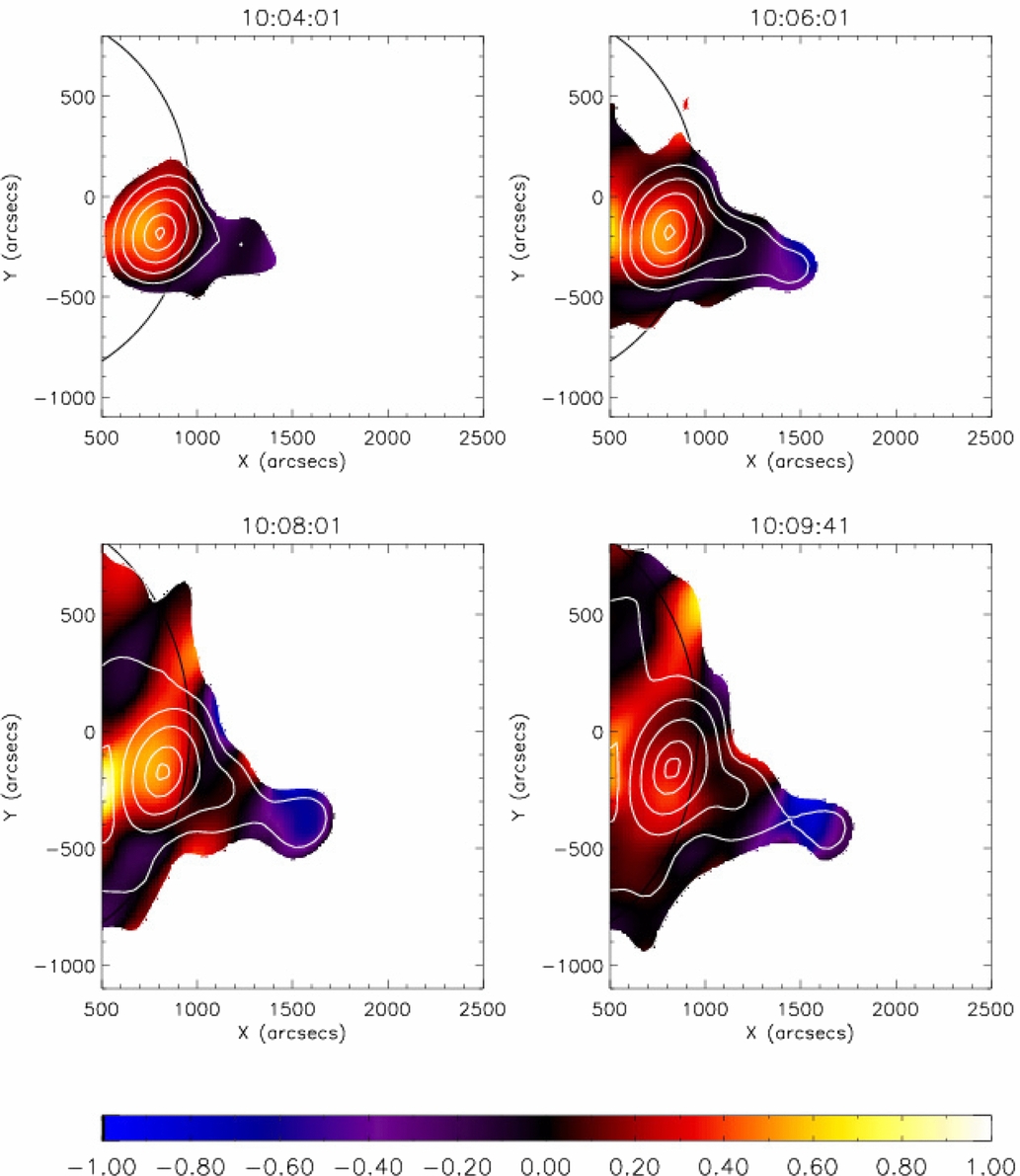
Figure 9 shows the degree of polarization, i.e., stokes V/I, for four snapshots during the burst at 228 MHz. White contours indicate the 4%, 8%, 16%, 32%, 64% and 96% levels of the maximum intensity in each radio map to delineate the noise storm and the propagating radio sources. We show only polarization data within the selected contours to avoid noise from low flux regions. Figure 10 shows the polarization as a function of time throughout the burst for source II at 150 MHz, 173 MHz and 228 MHz. At other frequencies the polarization data was unreliable. From Figure 10 we find that in general all three of the lowest NRH frequencies were around 40% polarized until around 10:12 UT, after which the degree of polarization at 150 MHz steadily increased to around 70%, while at 173 MHz and 228 MHz the degree of polarization slowly decreased over time.

Figure 9. NRH polarization images showing stokes V/I at 228 MHz. Plotted contours outline the intensity of the stokes I component at 4%, 8%, 16%, 32%, 64%, and 96%.
Download figure:
Standard image High-resolution image
Figure 10. Temporal evolution of the CME-RS source II stokes V/I polarization at 150 MHz (pink solid), 173 MHz (red dash-dotted) and 228 MHz (orange dashed).
Download figure:
Standard image High-resolution image4. PLASMA DIAGNOSTICS
Exact expressions for the gyrosynchrotron emissivity and absorption coefficient are complex (Ramaty 1969). Furthermore, as the spectrum observed with NRH does not show a turnover in the gyrosynchrotron spectrum, a unique fit to the data is not possible. Instead a range of source parameters can be recovered. First, an estimate of the source parameters can be obtained using the simplified semi-empirical approximations of Dulk & Marsh (1982) (and corrections in Dulk 1985), which assumes optically thin gyrosynchrotron emission from an isotropic pitch angle distribution. The approximations are valid for 10 ≳ ν/νB ≳ 100, 2 ⩽ δ ⩽ 7 and 20° ≳ θ ≳ 80°, but can suffer inaccuracies outside these specific parameter regimes. The results are then compared to simulated spectra using the more accurate gyrosynchrotron hybrid codes developed by Fleishman & Kuznetsov (2010).
4.1. Parameter Estimates using the Dulk & Marsh Semi-empirical Relations
Using the relation
from Dulk (1985), where rc is the degree of circular polarization, θ is the viewing angle of the observer with respect to the magnetic field and νB is the electron gyrofrequency (νB = eB/2πmec ≈ 2.8B MHz, where B is the magnetic field strength in units of Gauss), we can determine an estimate of B. Assuming θ ≈ 80° (since the CME-RS appears over the limb) and using δ = 4.9, ν = 150 MHz and rc ≈ 40% for source II at 10:09:41 UT, we find B ≈ 5.9 G. Furthermore, Razin-Tsytovich suppression can occur in a magnetized plasma when the effects of the medium become important and the refractive index is greater than 1 (Ginzburg & Syrovatskii 1965). When this occurs the emitted radiation becomes suppressed below the critical frequency νR
where νp is the local plasma frequency and ne is the ambient thermal electron density. Since no suppression is observed in the radio spectrum for source II, νR ≪ 150 MHz. From the LASCO WL CME observations we can determine the CME mass and in turn, estimate the electron density, ne in the CME core to be in the range 105–106 cm−3. This provides us with a lower limit on B of 0.01 G.
Using the relation

for optically thin plasma, where τ is the optical depth, Teff is the effective temperature, L the line of sight distance through the source and kB is Boltzmann's constant, with the Dulk (1985) relation for emissivity, η, expressed in terms of η/BN

where N is the non thermal electron density, and rearranging, we can determine N for electrons greater than E0 = 10 keV. Here E0 is the low electron energy cut off, with 10 keV being the value used in the determination of the semi-empirical formulae of Dulk (1985).

From radio imaging we estimate L ≈ 300'' ≈ 2 × 1010 cm, assuming the extent of source II along the line of sight is similar to its diameter in the plane of sky. Using B = 5.9 G, we find a nonthermal electron density, N, above 10 keV to be roughly 104 cm−3 (the lower limit of 0.01 G requires an unrealistically high nonthermal electron density, when compared to the thermal electron density).
4.2. Parameter Estimates using the Fleishman & Kuznetsov Gyrosynchrotron Code
It is known that parameters derived using the semi-empirical relations of Dulk (1985) can contain inaccuracies. We have therefore compared our observations with simulated spectra generated using fast gyrosynchrotron codes (see Fleishman & Kuznetsov (2010) for details) covering a large parameter space. Spectra were generated for a number of instances with varying values of B, N, θ, Emin and δ, and maps of the reduced χ2 produced. Figure 11 shows χ2 maps in the plane of B and N, for varying values of Emin (plots left to right) and θ (top to bottom). For all plots in Figure 11, we have imposed δ = 5, as determined from the fitted source II spectrum. Colored pixels are only shown for reduced χ2 values of less than 100 (shown to high values to highlight the mapping of χ2), while the remaining white space contains χ2 greater than 100. The colored pixels are normalized across the parameter space shown in the complete figure, not just to the values in each plot. Reasonable comparisons between the simulated spectra and the observed data start with χ2 < 7, corresponding to green pixels, however for our discussion we refer to only the lowest χ2 values corresponding to the red/orange pixels.

Figure 11. Maps showing the reduced χ2 comparisons between NRH spectra for source II and simulated spectra for various parameter combinations. Each panel shows the plane of B vs. N. Plots from left to right show increasing values for Emin and plots from top to bottom show a decreasing viewing angle, θ. All plots are for δ = 5. Only pixels with χ2 < 100 are colored, with red/orange pixels containing the lowest χ2 values of interest.
Download figure:
Standard image High-resolution imageWithout a turnover in the gyrosynchrotron spectrum, there exists a number of local minima that can provide a good fit to the observed spectrum, as is seen by the spatial variance of the red/orange pixels in each plot of Figure 11. We choose to show only a subset of the explored parameter space, limited to plots with typical values of Emin between 10 keV and 316 keV. This chosen range contains the lowest χ2 pixels for δ = 5, and the ranges of B and N examined. Each plot shows B in the range 1 to 20 G, based loosely on the expected value of B calculated above. A lower limit of 1 G is used as, below this value, the required nonthermal electron density to match the data approaches the estimated thermal electron density. Such a scenario is unlikely as this would require a very efficient acceleration mechanism.
Focusing on the top row of Figure 11 where θ = 80°, and assuming Emin = 10 keV, the best fit to the data requires N = 3.98 × 104 cm−3 with B = 3.7 G. For a source volume of 4.2 × 1030 cm−3, the total number of nonthermal electrons (above 10 keV) present in the source is then around 1.67 × 1035. This corresponds to a nonthermal electron energy content of 2.68 × 1027 erg. Applied similarly to Emin = 31.62 keV and 100 keV, Table 2 shows the resulting number of electrons within the source and the corresponding nonthermal energy content. For comparison, the thermal contribution to the source, with ne = 106 cm−3, contains around 1037 ambient electrons. Assuming a rough temperature estimate of 0.7 MK, i.e., the peak temperature response at 171 Å (O'Dwyer et al. 2010; Boerner et al. 2012) where the source was last observed in EUV a few minutes prior (we note that the source may have cooled during this period), gives a thermal energy of 1027 erg. It is therefore likely that the values in the first row of Table 2 are an upper limit to the number of nonthermal electrons and nonthermal energy content within source II. We also point out that the minimum χ2 in the bottom left plot for θ = 10° also requires an unrealistic nonthermal electron density of 106cm−3 to match the observed spectrum (Table 2, bottom row). In reality, θ is most likely varying throughout the source. This is evidenced in the AIA images which show the field to be highly twisted and change in orientation as the CME erupts, see Figure 2. While we cannot distinguish between several parameter combinations that match the data equally well, previous studies of gyrosynchrotron emission from CMEs have shown that the emission typically results from electrons in the range 100 keV to 1 MeV (Bastian et al. 2001). If we therefore assume a low energy cut off of several tens to 100 keV, the nonthermal energy content of source II is between 0.001% and 0.1% of the thermal energy content of the source.
Table 2. Input Parameters for the Simulated Gyrosynchrotron Spectra and the Resulting Nonthermal Energy Content
| δ | θ | Emin | B | N | No. of e− | |
|---|---|---|---|---|---|---|
| (°) | (keV) | (G) | (cm−3) | (erg) | ||
| 5 | 80 | 10.0 | 3.7 | 3.98 × 10⁴ | 1.67 × 1035 | 2.68 × 1027 |
| 5 | 80 | 31.6 | 3.7 | 3.98 × 10² | 1.67 × 1033 | 8.47 × 1025 |
| 5 | 80 | 100.0 | 3.7 | 3.98 | 1.67 × 1031 | 2.68 × 1024 |
| 5 | 10 | 10.0 | 5.2 | 3.98 × 10⁶ | 1.67 × 1037 | 2.68 × 1029 |

Download table as: ASCIITypeset image
For 10 keV electrons, the energy loss timescale by Coulomb collisions for a source with the value for ne estimated above is 4 hr (longer if you consider synchrotron energy loss alone) and over 49 hr at 100 keV to 1 MeV. Therefore a population of trapped accelerated electrons have the ability to explain the observed emission throughout the duration of the burst without needing to be replenished. However assuming the electrons are able to escape, the crossing time through the source is <1 s, which would require there to be a continued injection of accelerated electrons into the source.
The parameters recovered from this study are somewhat different to those found in a recent study by Tun & Vourlidas (2013). Firstly, the spectra presented in the Tun & Vourlidas (2013) paper shows a turnover at low frequencies which they attribute to gyrosynchrotron self-absorption. Our analysis shows no evidence of a turnover. Tun & Vourlidas (2013) finds B in the (slightly higher) range of 5–15 G and N = 2 × 106 cm−3. However, the Tun & Vourlidas (2013) study assumes an electron energy range of 1–100 keV and fitting the data, finds δ = 3. Alternatively, for the simulated spectra shown here, we set an upper limit for the electron energy to 10 MeV and varied the lower energy cutoff. We also impose the value δ = 5, which was found by fitting the radio spectrum with a power law to determine α, and using the Dulk (1985) approximation to determine δ. The choice of high energy cutoff can change the spectral slope of the fitted spectrum (Holman 2003) and may explain the discrepancy. Although not show in Figure 11, our parameter survey was extended to Emin = 1 keV, but this parameter range did not contain the minimum χ2 for the parameter space.
5. CONCLUSIONS
The radio observations presented in this paper are consistent with a moving type IV solar radio burst which is cospatial with the core of a propagating CME. As with previously documented type IV events, the source fragments into multiple sources, of which, we examined source II in detail. Like many type IV radio components, source II is moderately polarized (40% at the three lowest NRH observing frequencies) over the peak of the burst before steadily increasing to around 70% polarization at 150 MHz, though we note that the 173 MHz and 228 MHz channels show instead a steady decrease in polarization during the decay phase of the burst. Noise storm subtracted spectra for this source revealed a clear power law component with no turn over at low frequencies. Fits to the spectra found α to be in the range 3–5 throughout the burst for the type IVM source, which is consistent with optically thin nonthermal gyrosynchrotron emission.
To parameterize the underlying accelerated electron distribution and magnetic field, simulated gyrosynchrotron spectra were produced over a large parameter space. Without a turnover in the spectrum it was not possible to obtain a single set of parameters, as there exists several valid local χ2 minima within the parameter space. However making some reasonable assumptions about the source we find that the emission is likely produced by a nonthermal electron distribution with a density in the range 100–102 cm−3, in a magnetic field of several Gauss, with Emin around several tens to 100 keV. However, without accurate knowledge of the direction of the magnetic field it is not possible to determine whether the emission is x or o-mode. The nonthermal energy content of the source was found to be between 0.001% and 0.1% of the its thermal energy content. From estimates of the energy loss timescales, it is expected that the accelerated electrons would not thermalize for several hours. This suggests the electrons could have been accelerated early in the event, without the need to be replenished.
From the combined radio, white light and EUV observations presented in this paper, we find the type IVM source is associated with the core of the erupting CME. Previous papers in the literature have suggested that type IVM sources can be part of an expanding magnetic arch. In such a scenario it is likely that we are only observing the brightest part of the expanding flux rope associated with the CME, where a large number of nonthermal electrons are either accelerated or trapped in the structure. This could be the result of the observing instruments dynamic range. Furthermore, since gyrosynchrotron emission is a common feature of both the moving type IVM bursts and of the considerably rarer gyrosynchrotron CME features (Bastian et al. 2001; Maia et al. 2007; Démoulin et al. 2012), it is reasonable to suggest that these two phenomena could be related. In the later, gyrosynchrotron emission is seen at all points along the structure. This could be due to a more homogeneous source than in the case of a type IV, where the emission comes from fragmented sources along the structure. With new observations from the Low-Frequency Array (30–240 MHz; de Vos et al. 2009; van Haarlem et al. 2013), the Chinese Solar Radio Heliograph (0.4–15 GHz; Yan et al. 2009) and the proposed Frequency Agile Solar Radiotelescope (0.03–30 GHz; Gary & Keller 2004), it is hoped that many more such events will be observed and will allow us to directly investigate the relationship between these features for the first time.
This work was supported in part by the RHESSI project, NASA contract NAS598033. H.M.B. and S.K. were partially supported by the NASA grant NNX12AG98G.
The authors wish to thank the anonymous referee whose suggestions helped to improve the paper.