


ABSTRACT
We have determined astrometric positions for 15 WISE-discovered late-type brown dwarfs (six T8-9 and nine Y dwarfs) using the Keck-II telescope, the Spitzer Space Telescope, and the Hubble Space Telescope. Combining data from 8 to 20 epochs we derive parallactic and proper motions for these objects, which puts the majority within 15 pc. For ages greater than a few Gyr, as suggested from kinematic considerations, we find masses of 10–30 MJup based on standard models for the evolution of low-mass objects with a range of mass estimates for individual objects, depending on the model in question. Three of the coolest objects have effective temperatures ∼350 K and inferred masses of 10–15 MJup. Our parallactic distances confirm earlier photometric estimates and direct measurements and suggest that the number of objects with masses below about 15 MJup must be flat or declining, relative to higher mass objects. The masses of the coldest Y dwarfs may be similar to those inferred for recently imaged planet-mass companions to nearby young stars. Objects in this mass range, which appear to be rare in both the interstellar and protoplanetary environments, may both have formed via gravitational fragmentation—the brown dwarfs in interstellar clouds and companion objects in a protoplanetary disk. In both cases, however, the fact that objects in this mass range are relatively infrequent suggests that this mechanism must be inefficient in both environments.
1. INTRODUCTION
Our understanding of the gravitational collapse of interstellar gas clouds to form stars is one of the great success stories of modern astrophysics. The discovery of "protostars" in molecular clouds via infrared (IR) and millimeter observations started with high-luminosity stars in giant molecular clouds (e.g., the Becklin–Neugebauer (Becklin & Neugebauer 1967) and Kleinmann–Low (Kleinmann & Low 1967) objects in the Orion Molecular Cloud; Wilson et al. 1970) and progressed steadily through to the discovery of young stars of solar mass in clouds like Taurus (Beichman et al. 1986) and to objects of still lower masses with Spitzer (Dunham et al. 2013). The theory of star formation progressed hand in hand with observations, from initial discussions of the cloud collapse (Larson 1985) to detailed models incorporating disks and outflows (Shu et al. 1987). Long-standing questions in star formation theory concern the distribution of stellar masses (the initial mass function, IMF) produced by this process and the end points of the process (i.e., the largest and smallest self-gravitating objects that can be formed via gravitational collapse). The discovery of substellar objects, "brown dwarfs," orbiting nearby stars (Nakajima et al. 1995) and in early sky surveys—The Two Micron All sky survey (2MASS; Skrutskie et al. 2006), DEep Near Infrared Southern Sky Survey (Epchtein et al. 1997), and the Sloan Digital Sky Survey (SDSS; York et al. 2000)—pushed the low mass limit of the IMF well below the 0.07 M☉ stellar limit (Kirkpatrick et al. 1999; Kirkpatrick 2005). Data from the UKIRT Infrared Deep Sky Survey added many new L and T dwarfs and improved our knowledge of their space densities (Burningham et al. 2013). Most recently, the launch of the Wide-field Infrared Survey Explorer (WISE; Wright et al. 2010) has led to the identification of more than 250 brown dwarfs with extremely low effective temperatures, Teff, including the first Y dwarfs with Teff ∼ 250–500 K (Kirkpatrick et al. 2011, 2012; Cushing et al. 2011).
In the early 1980s, before the advent of theories of non-baryonic dark matter, it was thought that sharply increasing low-mass stellar and brown dwarf mass functions could account for the local missing mass inferred from galaxy rotation curves (Bahcall & Casertano 1985). This conjecture was ultimately ruled out as the shape of the low-mass IMF was determined with results from the Hubble Space Telescope (HST; Flynn et al. 1996), SDSS, and 2MASS, as well as by the incidence of microlensing events determined by the MACHO project (Alcock et al. 1996). Thus, while the low-mass shape of the IMF is no longer of cosmological importance, it remains an important question for star formation theory and the role of gravitational instability in the origin of the IMF. A related question about gravitational instability arises due to the existence of planetary mass companions on extremely wide orbits (e.g., HR 8799 and Fomalhaut; Marois et al. 2008; Kalas et al. 2004), which is difficult to reconcile with models of planet formation via core accretion (Dodson-Robinson et al. 2009). The formation of low-mass objects via gravitational instability also appears to be important in the protoplanetary environment.
Thus, we investigate Y dwarfs found with WISE as probes of the low-mass IMF and as analogs to the massive planets orbiting nearby stars. Our long-term goals are to understand better the physical properties of these objects and to assess how they might form, in either the interstellar or protoplanetary environments. A key step toward this goal is to determine the distances to the closest, lowest mass objects found by WISE. The first paper in this program reported a parallax for one of the coldest WISE Y dwarfs, WISE 1828+2650, classified as a ⩾Y2 object with a temperature of ∼300–500 K and a mass of ∼5 MJup for an assumed age of ∼5 Gyr (Beichman et al. 2013). We report here on parallax determinations of 15 WISE objects with spectral types of T8 or later, made using imaging from the HST, Spitzer Space Telescope, and Keck-II telescope. In what follows, we define the sample (Section 2), describe the observations (Section 3), and derive the kinematic parameters (Section 4). In Section 5 we use the spectral energy distribution (SED) and absolute magnitudes to estimate the masses of the Y dwarfs, address the possible ages of the sample objects on the basis of their kinematic properties, and discuss the apparent cutoffs in the distributions of brown dwarf and planetary companions in the range of <15 MJup.
2. THE SAMPLE
One of the key goals of the WISE mission was the detection of ultra-cool T and Y brown dwarfs with the properties of the instrument tailored such that the W2 filter at 4.6 μm was positioned to sit at the peak of the cool brown dwarf SED, while the shorter wavelength W1 filter at 3.5 μm sits in a region of methane absorption (Burrows et al. 1997). Thus, the prominent red W1 − W2 color of brown dwarfs makes them relatively easy to identify among the millions of WISE sources, so the objects studied in this paper (Table 1) are selected primarily for their extreme color, W1 − W2 > 2.5 mag (Kirkpatrick et al. 2011, 2012; Cushing et al. 2011, 2014; Mace et al. 2013). Approximately 17 Y dwarfs are presently known, including field objects from WISE, a T dwarf companion (Liu et al. 2012), and a white dwarf companion9 (Luhman et al. 2011). In this paper, we study nine WISE field Y dwarfs and six, slightly warmer, late T dwarfs.
Table 1. Astrometric Targets
| WISE Designation | Spectral Type | Sp. Ref | Detections (M/N)a | # Keck Obs. | # Hubble Obs. | # Spitzer Obs. | Baseline |
|---|---|---|---|---|---|---|---|
| (yr) | |||||||
| J014656.66+423410.0 (WISE 0146+42) | Y0 | 1 | 13/39 | 7 | 0 | 8 | 2.5 |
| J031325.94+780744.2 (WISE 0313+78) | T8.5 | 3 | 16/16 | 4 | 0 | 5 | 3.6 |
| J033515.01+431045.1 (WISE 0335+43) | T9 | 4 | 9/12 | 5 | 1 | 8 | 2.4 |
| J041022.71+150248.4 (WISE 0410+15) | Y0 | 2 | 12/12 | 2 | 1 | 11 | 2.3 |
| J071322.55−291751.9 (WISE 0713−29) | Y0 | 1 | 11/15 | 5 | 0 | 5 | 1.3 |
| J083641.10−185947.0 (WISE 0836−18) | T8p | 3 | 7/15 | 4 | 0 | 3 | 2.1 |
| J131106.20+012254.3 (WISE 1311+01) | T9: | 3 | 9/17 | 5 | 0 | 4 | 2.2 |
| J154151.65−225024.9 (WISE 1541−22) | Y0.5 | 2 | 10/10 | 4 | 2 | 4 | 2.1 |
| J154214.00+223005.2 (WISE 1542+22) | T9.5 | 4 | 22/45 | 1 | 2 | 3 | 1.8 |
| J173835.53+273259.0 (WISE 1738+27) | Y0 | 2 | 16/18 | 3 | 1 | 10 | 2.7 |
| J180435.37+311706.4 (WISE 1804+31) | T9.5: | 3 | 15/19 | 5 | 0 | 9 | 3.0 |
| J182831.08+265037.7 (WISE 1828+26) | ⩾Y2 | 1 | 12/18 | 5 | 4 | 11 | 2.9 |
| J205628.91+145953.2 (WISE 2056+14) | Y0 | 2 | 12/12 | 6 | 1 | 11 | 2.9 |
| J220905.73+271143.9 (WISE 2209+27) | Y1 | 5 | 13/15 | 4 | 1 | 6 | 2.4 |
| J222055.31−362817.4 (WISE 2220−36) | Y0 | 1 | 11/17 | 2 | 1 | 6 | 1.8 |
Notes. aNumber of actual detections, M, relative to number of possible detections, N in WISE W2 band. References. (1) Kirkpatrick et al. 2012; (2) Cushing et al. 2011; (3) Kirkpatrick et al. 2011; (4) Mace et al. 2013; (5) Cushing et al. 2014.
Download table as: ASCIITypeset image
As discussed in Kirkpatrick et al. (2012), we suggest that the Y dwarf sample is relatively complete at the WISE W2 magnitude limits appropriate to low ecliptic latitudes. While the V/Vmax value of 0.3 indicates that the late T and Y dwarf sample out to 10 pc are modestly incomplete (Kirkpatrick et al. 2012; Schmidt 1968), a number of investigations are underway to identify additional Y dwarfs with WISE, including improved processing and more follow-up observations. The sample studied here of nine Y dwarfs, limited only by a declination limit of δ > −36°, represents a large fraction of the available Y dwarfs from WISE. An additional six objects, late T dwarfs, were included in the sample to help to elucidate the transition between these two spectral types.
3. OBSERVATIONS
As described in Beichman et al. (2013), we piece together positional information with a variety of telescopes in the 1–5 μm range. In the near-IR, where the Y dwarfs are intrinsically faint, we used the Keck-II telescope with laser guide star adaptive optics (AO) and, for nine objects, the HST. In the 3–5 μm range, where the sources are much brighter, we have the original WISE measurements, which are of low positional accuracy, as well as Spitzer observations, which offer higher resolution and signal-to-noise ratio (S/N). Individual positional uncertainties with the various telescopes range between 5 and 10 mas (Keck and HST), 60 mas (Spitzer), and 250–500 mas (WISE). We tied together multiple astrometric reference frames, which adds an additional layer of positional uncertainty. While this multiplicity of telescopes presents the challenge of matching astrometric reference frames, we gain the advantage of a long temporal baseline and denser sampling of the Y dwarf motions that would be difficult to achieve with a single facility. Table 1 lists the WISE sources, their spectral types, and the number of observations with a particular facility. Table 2 gives the observing log for each facility as well the astrometric data at each epoch (Section 4).
Table 2. Observing Log and Astrometric Data
| WISE Designation | Observatory | Date | Filter | AOR | PI | MJD | R.A. | Decl. | Uncertainty |
|---|---|---|---|---|---|---|---|---|---|
| (UT) | (J2000) | (J2000) | (mas) | ||||||
| J014656.66+423410.0 | WISE | 2010 Jan 27 | 55223.14 | 26.7361144 | 42.5694586 | 250 | |||
| Spitzer | 2011 Apr 5 | Ch1 | 41808128 | Kirkpatrick | 55656.09 | 26.7359654 | 42.5694282 | 60 | |
| Spitzer | 2011 Apr 5 | Ch2 | 41808128 | Kirkpatrick | 55656.09 | 26.7359584 | 42.5693949 | 60 | |
| Keck | 2011 Dec 19 | H | Beichman | 55914.28 | 26.7358852 | 42.5694054 | 50 | ||
| Spitzer | 2012 Mar 7 | H | Beichman | 55993.04 | 26.7358141 | 42.5694177 | 60 | ||
| Spitzer | 2012 Mar 7 | Ch2 | 44544000 | Kirkpatrick | 55993.04 | 26.7358141 | 42.5694177 | 60 | |
| Spitzer | 2012 Oct 15 | Ch2 | 44588544 | Kirkpatrick | 56215.07 | 26.7358141 | 42.5694177 | 50 | |
| Keck | 2013 Jan 25 | H | Beichman | 56317.22 | 26.7356976 | 42.5694103 | 30 | ||
| Spitzer | 2013 Mar 13 | H | Beichman | 56364.25 | 26.7356437 | 42.5693903 | 60 | ||
| Spitzer | 2013 Mar 13 | Ch2 | 46549760 | Kirkpatrick | 56364.25 | 26.7356437 | 42.5693903 | 60 | |
| Spitzer | 2013 Mar 21 | Ch2 | 46549504 | Kirkpatrick | 56372.31 | 26.7356303 | 42.5694013 | 60 | |
| Spitzer | 2013 Apr 6 | Ch2 | 46549248 | Kirkpatrick | 56388.81 | 26.7356659 | 42.5693978 | 60 | |
| Spitzer | 2013 Apr 11 | Ch2 | 46548992 | Kirkpatrick | 56393.13 | 26.7356847 | 42.5693894 | 60 | |
| Keck | 2013 Sep 20 | H | Beichman | 56555.42 | 26.7356234 | 42.5694212 | 20 | ||
| Keck | 2013 Nov 19 | H | Beichman | 56615.29 | 26.7355696 | 42.569411 | 30 | ||
| J031358.93+780748.9 | WISE | 2010 Dec 21 | 55256.99 | 48.3581137 | 78.1289762 | 250 | |||
| WISE | 2010 Dec 21 | 55448.08 | 48.35846 | 78.1289878 | 250 | ||||
| Spitzer | 2010 Dec 21 | Ch1 | 41443840 | Kirkpatrick | 55551.35 | 48.3586706 | 78.1290368 | 60 | |
| Spitzer | 2010 Dec 21 | Ch2 | 41443840 | Kirkpatrick | 55551.35 | 48.3586761 | 78.1290121 | 60 | |
| Spitzer | 2011 Apr 23 | Ch2 | 41735936 | Kirkpatrick | 55674.71 | 48.3584757 | 78.128978 | 60 | |
| Keck | 2011 Oct 16 | H | Beichman | 55850.57 | 48.3588985 | 78.1290222 | 20 | ||
| Spitzer | 2011 Dec 2 | Ch2 | 44803072 | Kirkpatrick | 55897.22 | 48.3588009 | 78.1290122 | 60 | |
| Spitzer | 2012 Apr 24 | Ch2 | 44798464 | Kirkpatrick | 56041.15 | 48.3585303 | 78.1290161 | 60 | |
| Keck | 2012 Oct 7 | H | Beichman | 56207.51 | 48.3589982 | 78.1290526 | 20 | ||
| Keck | 2013 Jan 25 | H | Beichman | 56317.25 | 48.3587497 | 78.1290253 | 30 | ||
| Keck | 2013 Sep 20 | H | Beichman | 56555.53 | 48.3591015 | 78.129052 | 30 | ||
| J033515.01+431045.1 | WISE1 | 2010 Feb 15 | 55242.16 | 53.8125634 | 43.1791225 | 310 | |||
| WISE2 | 2010 Aug 27 | 55435.86 | 53.8127677 | 43.1791506 | 150 | ||||
| Spitzer | 2011 Apr 19 | Ch1 | 41838848 | Kirkpatrick | 55670.15 | 53.8129519 | 43.1789742 | 60 | |
| Spitzer | 2011 Apr 19 | Ch2 | 41838848 | Kirkpatrick | 55670.15 | 53.8129111 | 43.1789762 | 60 | |
| Spitzer | 2011 Nov 17 | Ch2 | 44573696 | Kirkpatrick | 55882.78 | 53.8131682 | 43.1788608 | 60 | |
| Keck | 2012 Oct 7 | H | Beichman | 56207.59 | 53.8134114 | 43.17867 | 20 | ||
| Spitzer | 2012 Nov 22 | Ch2 | 46436096 | Kirkpatrick | 56253.19 | 53.8134568 | 43.1786443 | 60 | |
| Keck | 2012 Nov 29 | H | Beichman | 56260.38 | 53.8134285 | 43.1786345 | 20 | ||
| Keck | 2013 Jan 25 | H | Beichman | 56317.32 | 53.8134738 | 43.1785834 | 20 | ||
| HST | 2013 Mar 29 | F125W | Cushing | 56380.74 | 53.8135311 | 43.1785361 | 20 | ||
| Spitzer | 2013 Apr 7 | Ch2 | 46595328 | Kirkpatrick | 56389.02 | 53.8135567 | 43.178527 | 60 | |
| Spitzer | 2013 Apr 17 | Ch2 | 46595072 | Kirkpatrick | 56399.8 | 53.8135846 | 43.1785371 | 60 | |
| Spitzer | 2013 Apr 22 | Ch2 | 46594816 | Kirkpatrick | 56404.5 | 53.8135702 | 43.1785451 | 60 | |
| Spitzer | 2013 May 5 | Ch2 | 46594560 | Kirkpatrick | 56417.21 | 53.8135371 | 43.1785424 | 60 | |
| Keck | 2013 Sep 20 | H | Beichman | 56555.56 | 53.813732 | 43.1784515 | 20 | ||
| Keck | 2013 Nov 19 | H | Beichman | 56615.32 | 53.813756 | 43.1784148 | 20 | ||
| J041022.71+150248.4 | WISE | 2010 Feb 16 | 55243.6 | 62.5946547 | 15.046819 | 250 | |||
| WISE | 2010 Aug 26 | 55434.09 | 62.594941 | 15.0464875 | 250 | ||||
| Spitzer | 2010 Oct 21 | Ch1 | 40828160 | Kirkpatrick | 55490.06 | 62.5949777 | 15.0464452 | 55 | |
| Spitzer | 2010 Oct 21 | Ch2 | 40828160 | Kirkpatrick | 55490.06 | 62.5949953 | 15.0464292 | 55 | |
| Spitzer | 2011 Apr 14 | Ch2 | 41442304 | Kirkpatrick | 55665.88 | 62.5950177 | 15.0460896 | 55 | |
| HST | 2012 Sep 1 | F140W | Cushing | 56171.83 | 62.5954954 | 15.0452734 | 20 | ||
| Spitzer | 2011 Nov 19 | Ch2 | 44567808 | Kirkpatrick | 55884.56 | 62.5952786 | 15.0457531 | 55 | |
| Spitzer | 2011 Nov 24 | Ch1 | 44508160 | Dupuy | 55889.76 | 62.5952814 | 15.0457285 | 55 | |
| Spitzer | 2012 Mar 29 | Ch1 | 44508416 | Dupuy | 56015.06 | 62.5952928 | 15.0455135 | 55 | |
| Spitzer | 2012 Mar 30 | Ch2 | 44564480 | Kirkpatrick | 56016.76 | 62.5952956 | 15.0455307 | 55 | |
| Spitzer | 2012 Apr 29 | Ch1 | 44508672 | Dupuy | 56046.9 | 62.5953018 | 15.0454548 | 55 | |
| Spitzer | 2012 Oct 30 | Ch1 | 44508672 | Dupuy | 56230.96 | 62.5955446 | 15.0451638 | 55 | |
| Spitzer | 2012 Nov 19 | Ch2 | 46443008 | Kirkpatrick | 56250.9 | 62.595579 | 15.0451303 | 55 | |
| Spitzer | 2012 Nov 30 | Ch2 | 46442752 | Kirkpatrick | 56261.93 | 62.5955494 | 15.0451248 | 55 | |
| Keck | 2013 Jan 25 | H | Beichman | 56317.28 | 62.5955394 | 15.0450125 | 40 | ||
| Keck | 2013 Feb 20 | H | Beichman | 56343.24 | 62.5955423 | 15.0449683 | 20 | ||
| J071322.55−291751.9 | WISE | 2010 Apr 9 | 55296.64 | 108.3439684 | −29.2977331 | 160 | |||
| WISE | 2010 Oct 18 | 55488.21 | 108.3441041 | −29.2978282 | 200 | ||||
| Keck | 2011 Oct 16 | H | Beichman | 55850.64 | 108.3442071 | −29.2979174 | 30 | ||
| Spitzer | 2012 Jan 2 | Ch1 | 44568064 | Kirkpatrick | 55928.89 | 108.344187 | −29.2979651 | 80 | |
| Spitzer | 2012 Jan 2 | Ch2 | 44568064 | Kirkpatrick | 55928.89 | 108.3442477 | −29.2979653 | 55 | |
| Keck | 2012 Mar 31 | H | Beichman | 56017.24 | 108.3441896 | −29.2979665 | 30 | ||
| Keck | 2012 Oct 7 | H | Beichman | 56207.63 | 108.3443149 | −29.2980289 | 30 | ||
| Spitzer | 2012 Dec 25 | Ch2 | 46439936 | Kirkpatrick | 56286.71 | 108.3443274 | −29.2980777 | 55 | |
| Spitzer | 2013 Jan 17 | Ch2 | 46439680 | Kirkpatrick | 56309.98 | 108.3443808 | −29.2980687 | 55 | |
| Keck | 2013 Jan 25 | H | Beichman | 56317.35 | 108.3443186 | −29.2980846 | 20 | ||
| Spitzer | 2013 Feb 6 | Ch2 | 46439424 | Kirkpatrick | 56329.14 | 108.3443683 | −29.2981035 | 55 | |
| Keck | 2013 Feb 20 | H | Beichman | 56343.28 | 108.3443092 | −29.2980885 | 30 | ||
| J083641.10−185947.0 | WISE | 2010 May 2 | 55319.67 | 129.1712834 | −18.9963895 | 1000 | |||
| WISE | 2010 Nov 10 | 55510.55 | 129.1714539 | −18.996376 | 1220 | ||||
| Spitzer | 2011 Jan 1 | Ch2 | 40833536 | Kirkpatrick | 55563 | 129.1715552 | −18.9962973 | 50 | |
| Spitzer | 2011 May 31 | Ch2 | 41701888 | Kirkpatrick | 55712.03 | 129.1715494 | −18.9963169 | 50 | |
| Spitzer | 2012 Jan 17 | Ch2 | 44556032 | Kirkpatrick | 55943.76 | 129.1715477 | −18.9963443 | 50 | |
| Keck | 2012 Nov 29 | H | Beichman | 56260.57 | 129.1715439 | −18.9963665 | 30 | ||
| Keck | 2013 Jan 25 | H | Beichman | 56317.41 | 129.17153 | −18.9963856 | 20 | ||
| Keck | 2013 Feb 20 | H | Beichman | 56343.33 | 129.1715283 | −18.9963813 | 20 | ||
| Keck | 2013 Nov 19 | H | Beichman | 56615.59 | 129.1715276 | −18.996414 | 20 | ||
| J131106.20+012254.3 | WISE | 2010 Jan 9 | 55206.33 | 197.7760137 | 1.3817997 | 350 | |||
| WISE | 2010 Jul 2 | 55380.12 | 197.7759224 | 1.3817217 | 340 | ||||
| Spitzer | 2011 Mar 29 | Ch1 | 40826368 | Kirkpatrick | 55649.37 | 197.7761222 | 1.3814907 | 60 | |
| Spitzer | 2011 Mar 29 | Ch2 | 40826368 | Kirkpatrick | 55649.37 | 197.7760981 | 1.3815201 | 60 | |
| Spitzer | 2012 Mar 29 | Ch2 | 44575232 | Kirkpatrick | 56015.51 | 197.7762172 | 1.3812636 | 60 | |
| Keck | 2012 Mar 31 | H | Beichman | 56017.4 | 197.7761705 | 1.3812709 | 30 | ||
| Keck | 2012 Jul 9 | H | Beichman | 56117.26 | 197.7761937 | 1.3812213 | 30 | ||
| Spitzer | 41143 | Ch2 | 44571904 | Kirkpatrick | 56161.13 | 197.7761852 | 1.3811918 | 50 | |
| Keck | 2013 Jan 25 | H | Beichman | 56317.5 | 197.7762561 | 1.3810702 | 30 | ||
| Keck | 2013 Feb 20 | H | Beichman | 56343.45 | 197.776254 | 1.3810576 | 20 | ||
| Keck | 2013 May 27 | H | Beichman | 56439.25 | 197.7762548 | 1.3810158 | 20 | ||
| J154151.65−225024.9 | WISE | 2010 Feb 16 | 55244.84 | 235.4651965 | −22.840523 | 500 | |||
| Spitzer | 2011 Apr 13 | Ch1 | 41788672 | Kirkpatrick | 55664.91 | 235.4648435 | −22.8404433 | 66 | |
| Spitzer | 2011 Apr 13 | Ch2 | 41788672 | Kirkpatrick | 55664.91 | 235.4648328 | −22.8404443 | 60 | |
| WISE | 2010 Aug 15 | 55424 | 235.4650457 | −22.8400781 | 500 | ||||
| Spitzer | 2012 Apr 22 | Ch1 | 44512512 | Dupuy | 56039.24 | 235.4645941 | −22.8404542 | 80 | |
| Spitzer | 2012 Apr 28 | Ch2 | 44550144 | Kirkpatrick | 56045.83 | 235.4646137 | −22.840462 | 60 | |
| Keck | 2012 Mar 31 | H | Beichman | 56017.51 | 235.464582 | −22.840456 | 20 | ||
| Spitzer | 2012 May 19 | Ch1 | 44512768 | Dupuy | 56066.22 | 235.464575 | −22.8404522 | 85 | |
| Keck | 2012 Jul 9 | H | Beichman | 56117.28 | 235.464431 | −22.840446 | 20 | ||
| Keck | 2013 Jan 25 | H | Beichman | 56317.63 | 235.4643821 | −22.840476 | 20 | ||
| HST | 2013 Feb 12 | F125W | Cushing | 56335.74 | 235.4643635 | −22.8404761 | 20 | ||
| HST | 2013 May 9 | F105W | Cushing | 56421.55 | 235.4642595 | −22.8404771 | 20 | ||
| Keck | 2013 May 27 | H | Beichman | 56439.33 | 235.4642458 | −22.8404802 | 20 | ||
| J154214.00+223005.2 | WISE | 2010 Feb 4 | 55232.37 | 235.558604 | 22.5015172 | 400 | |||
| WISE | 2010 Aug 3 | 55412.02 | 235.5583999 | 22.5015432 | 400 | ||||
| Spitzer | 2011 Apr 18 | Ch1 | 41058816 | Kirkpatrick | 55669.41 | 235.5579949 | 22.5013517 | 60 | |
| Spitzer | 2011 Apr 18 | Ch2 | 41058816 | Kirkpatrick | 55669.41 | 235.5580421 | 22.5013728 | 60 | |
| Spitzer | 2012 Apr 15 | Ch2 | 44559616 | Kirkpatrick | 56032.02 | 235.5577765 | 22.5012418 | 60 | |
| HST | 2012 Mar 4 | F140W | Kirkpatrick | 55990.91 | 235.5577799 | 22.5012605 | 15 | ||
| Spitzer | 2012 Sep 21 | Ch2 | 44557568 | Kirkpatrick | 56191.18 | 235.5575565 | 22.5012083 | 60 | |
| HST | 2013 Feb 13 | F125W | Cushing | 56336.82 | 235.557504 | 22.5011602 | 15 | ||
| Keck | 2013 Feb 20 | H | Beichman | 56343.52 | 235.5575356 | 22.5011738 | 60 | ||
| J173835.53+273259.0 | WISE | 2010 Mar 13 | 55269.03 | 264.6480543 | 27.5496933 | 250 | |||
| Spitzer | 2010 Sep 18 | Ch1 | 40828416 | Kirkpatrick | 55457.58 | 264.6480843 | 27.549658 | 50 | |
| Spitzer | 2010 Sep 18 | Ch2 | 40828416 | Kirkpatrick | 55457.58 | 264.6480788 | 27.5496439 | 50 | |
| WISE | 2010 Sep 9 | 55448.65 | 264.6481684 | 27.5496833 | 250 | ||||
| HST | 2011 May 12 | F140W | Kirkpatick | 55693.81 | 264.6481914 | 27.5495878 | 15 | ||
| Spitzer | 2011 May 20 | Ch2 | 41515264 | Kirkpatrick | 55701.63 | 264.6482049 | 27.549556 | 50 | |
| Spitzer | 2011 Nov 26 | Ch2 | 41515264 | Kirkpatrick | 55891.28 | 264.648178 | 27.5495077 | 50 | |
| Keck | 2012 Mar 31 | H | Beichman | 56017.55 | 264.6482856 | 27.5495029 | 25 | ||
| Spitzer | 2012 May 8 | Ch1 | 44513536 | Dupuy | 56055.9 | 264.6482997 | 27.549458 | 50 | |
| Spitzer | 2012 May 12 | Ch2 | 44558336 | Kirkpatrick | 56059.9 | 264.6483229 | 27.5494919 | 50 | |
| Keck | 2012 Jul 9 | H | Beichman | 56117.26 | 264.6482643 | 27.5495025 | 30 | ||
| Spitzer | 2012 Jul 10 | Ch1 | 44513792 | Dupuy | 56118.85 | 264.6483209 | 27.5494664 | 50 | |
| Spitzer | 2012 Sep 27 | Ch1 | 44513024 | Dupuy | 56197.4 | 264.6482847 | 27.5494635 | 50 | |
| Spitzer | 2012 Nov 19 | Ch2 | 46437888 | Kirkpatrick | 56250.73 | 264.6482591 | 27.5494299 | 50 | |
| Spitzer | 2012 Nov 27 | Ch1 | 44513280 | Dupuy | 56258.77 | 264.6482799 | 27.5494348 | 50 | |
| Keck | 2013 May 27 | H | Beichman | 56439.43 | 264.6483932 | 27.5494055 | 30 | ||
| J180435.37+311706.4 | WISE | 2010 Mar 21 | 55277.1 | 271.1472306 | 31.2851638 | 340 | |||
| WISE | 2010 Nov 9 | 55509.91 | 271.1471832 | 31.2852385 | 280 | ||||
| Spitzer | 2010 Sep 26 | Ch1 | 40836352 | Kirkpatrick | 55465.2 | 271.1472408 | 31.2851226 | 50 | |
| Spitzer | 2010 Sep 26 | Ch2 | 40836352 | Kirkpatrick | 55465.2 | 271.1472431 | 31.2851484 | 50 | |
| Spitzer | 2011 May 25 | Ch2 | 41565696 | Kirkpatrick | 55706.84 | 271.1472367 | 31.2851427 | 50 | |
| Spitzer | 2011 Nov 29 | Ch2 | 44571136 | Kirkpatrick | 55894.05 | 271.14717 | 31.2851347 | 50 | |
| Keck | 2012 Jul 9 | H | Beichman | 56117.37 | 271.1470991 | 31.2851768 | 30 | ||
| Spitzer | 2011 Dec 1 | Ch1 | 44515328 | Dupuy | 55896.97 | 271.1471423 | 31.2851566 | 50 | |
| Spitzer | 2012 May 16 | Ch1 | 44515584 | Dupuy | 56063.73 | 271.147159 | 31.2851443 | 50 | |
| Spitzer | 2012 May 16 | Ch2 | 44515584 | Dupuy | 56063.75 | 271.1471621 | 31.2851558 | 50 | |
| Spitzer | 2012 Jul 25 | Ch1 | 44515840 | Dupuy | 56133.39 | 271.1471254 | 31.2851738 | 50 | |
| Spitzer | 2012 Oct 3 | Ch1 | 44515072 | Dupuy | 56203.43 | 271.1470927 | 31.2851711 | 50 | |
| Keck | 2013 Apr 22 | H | Beichman | 56404.53 | 271.1470676 | 31.2851603 | 20 | ||
| Keck | 2013 May 27 | H | Beichman | 56439.4 | 271.147049 | 31.2851677 | 20 | ||
| J182831.08+265037.7 | WISE1 | 2010 Mar 30 | 55285.66 | 277.1295162 | 26.8438 | 170 | |||
| WISE | 2010 Sep 28 | 55467.55 | 277.1295247 | 26.8439192 | 210 | ||||
| Keck | 2010 Jul 1 | H | Beichman | 55378.44 | 277.1296241 | 26.8438953 | 100 | ||
| Spitzer | 2010 Jul 10 | Ch1 | 39526656 | Mainzer | 55387.29 | 277.1296029 | 26.8438554 | 60 | |
| Spitzer | 2010 Jul 10 | Ch2 | 39526656 | Mainzer | 55387.34 | 277.1296042 | 26.8438808 | 60 | |
| Spitzer | 2010 Dec 4 | Ch2 | 41027328 | Kirkpatrick | 55534.27 | 277.1296675 | 26.8438286 | 60 | |
| HST | 2011 May 9 | F140W | Kirkpatrick | 55690.89 | 277.1298806 | 26.8439048 | 30 | ||
| Keck | 2011 Oct 16 | H | Beichman | 55850.21 | 277.1299543 | 26.8439071 | 10 | ||
| Spitzer | 2011 Nov 29 | Ch2 | 44586752 | Kirkpatrick | 55894.04 | 277.1300176 | 26.8438958 | 60 | |
| Spitzer | 2011 Dec 2 | Ch1 | 44516352 | Dupuy | 55897.48 | 277.1300065 | 26.8439088 | 60 | |
| Spitzer | 2012 May 25 | Ch1 | 44516608 | Dupuy | 56072.2 | 277.1302159 | 26.8439439 | 60 | |
| Spitzer | 2012 May 25 | Ch2 | 44516608 | Dupuy | 56072.25 | 277.1301923 | 26.8439382 | 60 | |
| Keck | 2012 Jul 9 | H | Beichman | 56117.32 | 277.1302146 | 26.8439617 | 10 | ||
| Spitzer | 2012 Jul 23 | Ch1 | 44516864 | Dupuy | 56131.04 | 277.1302484 | 26.8439671 | 60 | |
| Keck | 2012 Oct 7 | H | Beichman | 56207.22 | 277.1302611 | 26.8439344 | 50 | ||
| Spitzer | 2012 Oct 18 | Ch2 | 44516096 | Dupuy | 56218.2 | 277.1302737 | 26.84398 | 60 | |
| Spitzer | 2012 Nov 18 | Ch2 | 46439168 | Kirkpatrick | 56249.43 | 277.1302789 | 26.8439821 | 60 | |
| Spitzer | 2012 Dec 8 | Ch2 | 46438912 | Kirkpatrick | 56269.92 | 277.1303385 | 26.8439822 | 60 | |
| HST | 2013 Apr 22 | F105W | Cushing | 56404.88 | 277.1305007 | 26.8439937 | 10 | ||
| HST | 2013 May 6 | F125W | Cushing | 56418.83 | 277.1305121 | 26.844001 | 10 | ||
| HST | 2013 May 8 | F105W | Cushing | 56420.76 | 277.13051 | 26.8440029 | 10 | ||
| Keck | 2013 May 27 | H | Beichman | 56439.36 | 277.1305206 | 26.8440076 | 10 | ||
| J205628.91+145953.2 | WISE-1 | 2010 May 13 | 55329.29 | 314.1204976 | 14.9981178 | 290 | |||
| Keck | 2010 Jul 1 | H | Beichman | 55378.6 | 314.1204617 | 14.9981905 | 30 | ||
| WISE | 2010 Nov 8 | 55514.2 | 314.1204976 | 14.9981178 | 290 | ||||
| Spitzer | 2010 Dec 10 | Ch1 | 40836608 | Kirkpatrick | 55540.03 | 314.1205267 | 14.9982425 | 60 | |
| Spitzer | 2010 Dec 10 | Ch2 | 40836608 | Kirkpatrick | 55540.03 | 314.1205241 | 14.998241 | 60 | |
| Spitzer | 2011 Jul 6 | Ch2 | 41831424 | Kirkpatrick | 55748.1 | 314.1207526 | 14.9983505 | 60 | |
| HST | 2011 Sep 5 | F140W | Kirkpatrick | 55808.36 | 314.1207034 | 14.9983548 | 20 | ||
| Keck | 2011 Oct 16 | H | Beichman | 55850.35 | 314.1207055 | 14.9983614 | 20 | ||
| Keck | 2011 Dec 19 | H | Beichman | 55914.2 | 314.1207544 | 14.9983705 | 40 | ||
| Spitzer | 2012 Jan 6 | Ch2 | 44573184 | Kirkpatrick | 55932.56 | 314.1207682 | 14.998396 | 60 | |
| Spitzer | 2012 Jan 22 | Ch1 | 44517376 | Dupuy | 55948.98 | 314.1207601 | 14.9983875 | 60 | |
| Keck | 2012 Jul 9 | H | Beichman | 56117.46 | 314.1209349 | 14.9984907 | 20 | ||
| Spitzer | 2012 Jul 10 | Ch1 | 44517632 | Dupuy | 56118.83 | 314.1209268 | 14.9984825 | 60 | |
| Keck | 2012 Oct 7 | H | Beichman | 56207.28 | 314.120941 | 14.9985341 | 50 | ||
| Spitzer | 2012 Jul 18 | Ch2 | 44569600 | Kirkpatrick | 56126.76 | 314.1209601 | 14.9984791 | 60 | |
| Spitzer | 2012 Aug 21 | Ch1 | 44517888 | Dupuy | 56160.05 | 314.1209851 | 14.9984985 | 60 | |
| Spitzer | 2012 Dec 22 | Ch2 | 46464000 | Kirkpatrick | 56283.4 | 314.1209624 | 14.9985174 | 60 | |
| Spitzer | 2013 Jan 4 | Ch2 | 46463488 | Kirkpatrick | 56296.19 | 314.1210188 | 14.9985212 | 60 | |
| Spitzer | 2013 Jan 22 | Ch2 | 46462720 | Kirkpatrick | 56314.75 | 314.1210053 | 14.9985509 | 60 | |
| Keck | 2013 May 27 | H | Beichman | 56439.46 | 314.1211613 | 14.998618 | 20 | ||
| J220905.73+271143.9 | WISE | 2010 Jun 6 | 55354.86 | 332.2739012 | 27.1955919 | 250 | |||
| Spitzer | 2010 Dec 31 | Ch2 | 40821248 | Kirkpatrick | 55561.94 | 332.2740681 | 27.1953371 | 60 | |
| Keck | 2011 Jul 20 | H | Beichman | 55762.5 | 332.2743368 | 27.1951698 | 30 | ||
| Spitzer | 2011 Jul 27 | Ch2 | 41698816 | Kirkpatrick | 55769.86 | 332.2743509 | 27.1951224 | 60 | |
| Spitzer | 2012 Jan 14 | Ch2 | 44548352 | Kirkpatrick | 55940.6 | 332.2744675 | 27.1949265 | 60 | |
| Keck | 2012 Jul 9 | H | Beichman | 56117.52 | 332.2747063 | 27.1948078 | 30 | ||
| Keck | 2012 Oct 7 | H | Beichman | 56207.32 | 332.2747329 | 27.1946743 | 30 | ||
| HST | 2012 Sep 15 | F140W | Cushing | 56185.58 | 332.2747399 | 27.1947115 | 20 | ||
| Spitzer | 2013 Jan 10 | Ch2 | 46543616 | Kirkpatrick | 56302.15 | 332.2748377 | 27.1945693 | 60 | |
| Spitzer | 2013 Jan 31 | Ch2 | 46543360 | Kirkpatrick | 56323.38 | 332.2748291 | 27.1945492 | 60 | |
| Spitzer | 2013 Feb 14 | Ch2 | 46543104 | Kirkpatrick | 56337.87 | 332.2748893 | 27.1945119 | 60 | |
| Keck | 2013 May 27 | H | Beichman | 56439.53 | 332.2750607 | 27.1944435 | 20 | ||
| J222055.31−362817.4 | WISE | 2010 May 14 | 55330.96 | 335.2304846 | −36.4713796 | 332 | |||
| WISE | 2010 Nov 9 | 55509.91 | 335.23058743 | −36.4715195 | 281 | ||||
| Spitzer | 2012 Jan 23 | Ch1 | 44552448 | Kirkpatrick | 55949.11 | 335.23056511 | −36.4715078 | 60 | |
| Spitzer | 2012 Jan 23 | Ch2 | 44552448 | Kirkpatrick | 55949.11 | 335.23056635 | −36.4715455 | 60 | |
| Spitzer | 2012 Jul 15 | Ch2 | 44574464 | Kirkpatrick | 56123.9 | 335.23068028 | −36.4715003 | 60 | |
| HST | 2012 Nov 23 | F125W | Cushing | 56254.33 | 335.23066052 | −36.4715666 | 20 | ||
| Spitzer | 2012 Dec 24 | Ch2 | 46460928 | Kirkpatrick | 56285.09 | 335.23068603 | −36.471558 | 60 | |
| Spitzer | 2013 Jan 6 | Ch2 | 46460160 | Kirkpatrick | 56298.03 | 335.23065602 | −36.4715587 | 60 | |
| Spitzer | 2013 Jan 26 | Ch2 | 46459392 | Kirkpatrick | 56318.93 | 335.2307343 | −36.4715553 | 60 | |
| Keck | 2013 Sep 21 | H | Beichman | 56556.32 | 335.23076402 | −36.4715891 | 10 | ||
| Keck | 2013 Nov 19 | H | Beichman | 56615.2 | 335.2307524 | −36.4715821 | 10 | ||
3.1. WISE Observations
The WISE mission had three distinct phases: the four-band cryogenic period, the three-band cryogenic period, and two-band warm mission. Depending on the position on the sky, especially ecliptic longitude, sources were observed in one or more of these phases. We determined positions and magnitudes for each period separately with a median date of observation spanning one to two days. Positions and associated uncertainties were obtained by averaging the source positions in the multi-band extractions from each individual orbit. The uncertainty in the WISE astrometric frame is approximately 80 mas, based on the input 2MASS catalog used for WISE position reconstruction (Cutri et al. 2011). Typically, however, the positional uncertainties in the WISE detections are much larger than this, ∼250–500 mas, due to its large beamsize and detection at only one, or at most two, wavelengths or to the effects of confusion with other nearby objects.
In Table 3 we report averages of the 4.5 μm magnitudes (W2) for the various epochs and include 3.5 μm (W1) when available. Upper limits in the two longer wavelength bands, 12 (W3) and 22 μm (W4), are high and do not significantly constrain the SEDs. We converted the magnitudes to flux densities using the zero points from Wright et al. (2010), but because of the unknown and extremely non-blackbody-like nature of brown dwarf SEDs, we have not color-corrected these flux densities. Table 4 indicates that there is no evidence for variability in the [4.6] mag at the 2%–3% level for any of these objects. While not varying in the Spitzer bands, WISE 2220−3628 shows evidence for variability in the comparison of the ground-based J and HST/F125W photometry, with a nearly 1 mag difference between the two bands. Further monitoring of this object may be warranted.
Table 3. Photometric Data (Magnitudes)
| WISE Designation | F105W | J | F125W | F140W | Ha | WISE [3.35] | Spitzer [3.6] | Spitzer [4.5] | WISE [4.6] |
|---|---|---|---|---|---|---|---|---|---|
| J014656.66+423410.0 | 19.40 ± 0.25b | 20.91 ± 0.21 | >18.99 | 17.42 ± 0.05 | 15.05 ± 0.03 | 15.08 ± 0.068 | |||
| J031325.94+780744.2 | 17.67 ± 0.07b | 17.67 ± 0.07 | 15.87 ± 0.058 | 15.31 ± 0.05 | 13.23 ± 0.03 | 13.18 ± 0.03 | |||
| J033515.01+431045.1 | 20.07 ± 0.30c | 20.23 ± 0.05 | 19.76 ± 0.13 | >18.15 | 16.58 ± 0.05 | 14.39 ± 0.03 | 14.60 ± 0.08 | ||
| J041022.71+150248.4 | 19.44 ± 0.03d | 19.74 ± 0.03 | 20.02 ± 0.05d | >18.25 | 16.62 ± 0.05 | 14.10 ± 0.03 | 14.18 ± 0.055 | ||
| J071322.55−291751.9 | 19.64 ± 0.15b | 19.85 ± 0.05 | >18.35 | 16.67 ± 0.05 | 14.22 ± 0.03 | 14.48 ± 0.06 | |||
| J083641.10−185947.0 | 18.99 ± 0.22c | 19.49 ± 0.24 | >18.41 | 16.85 ± 0.05 | 15.06 ± 0.03 | 15.18 ± 0.098 | |||
| J131106.20+012254.3 | 18.75 ± 0.07e | 19.09 ± 0.07 | >18.27 | 16.81 ± 0.05 | 14.64 ± 0.03 | 14.76 ± 0.086 | |||
| J154151.65−225024.9 | 21.41 ± 0.01 | 21.12 ± 0.06d | 21.69 ± 0.05 | 21.54 ± 0.11 | 16.74 ± 0.16 | 16.70 ± 0.05 | 14.21 ± 0.03 | 14.26 ± 0.06 | |
| J154214.00+223005.2 | 20.25 ± 0.13c | 20.73 ± 0.03 | 20.46 ± 0.03 | 20.34 ± 0.06 | >18.88 | 17.27 ± 0.05 | 15.02 ± 0.03 | 15.02 ± 0.06 | |
| J173835.53+273259.0 | 20.05 ± 0.09d | 19.89 ± 0.05 | 20.45 ± 0.09d | >18.40 | 16.94 ± 0.05 | 14.49 ± 0.03 | 14.55 ± 0.06 | ||
| J180435.37+311706.4 | 18.67 ± 0.04f | 19.21 ± 0.11b | >18.64 | 16.55 ± 0.05 | 14.59 ± 0.03 | 14.74 ± 0.06 | |||
| J182831.08+265037.7 | 23.96 ± 0.10 | 23.57 ± 0.35g | 23.83 ± 0.05 | 23.36 ± 0.05 | 22.45 ± 0.08g | >18.47 | 16.88 ± 0.05 | 14.30 ± 0.03 | 14.39 ± 0.06 |
| J205628.91+145953.2 | 19.43 ± 0.04d | 19.57 ± 0.04 | 19.96 ± 0.04d | >18.25 | 16.07 ± 0.05 | 13.92 ± 0.03 | 13.98 ± 0.05 | ||
| J220905.73+271143.9 | 22.58 ± 0.14h | 23.17 ± 0.03 | 22.98 ± 0.31h | >18.47 | N/A | 14.71 ± 0.03 | 14.79 ± 0.07 | ||
| J222055.31−362817.4 | 20.38 ± 0.17b | 21.21 ± 0.05 | 20.81 ± 0.30b | >18.65 | 17.17 ± 0.05 | 14.75 ± 0.03 | 14.66 ± 0.06 |
Notes. aUnless otherwise noted, H-band photometry is from NIRC2 from observations reported here. Photometry is on the MKO-NIR system. bKirkpatrick et al. (2012). cMace et al. (2013). dLeggett et al. (2013). eKirkpatrick et al. (2011). fUnpublished Palomar WIRC data. gBeichman et al. (2013). hCushing et al. (2014).
Download table as: ASCIITypeset image
Table 4. Spitzer Photometric Variability (Channel 2)
| WISE Designation | # Observations | σpop |
|---|---|---|
| (mag) | ||
| J014656.66+423410.0 | 7 | 0.013 |
| J031325.94+780744.2 | 4 | 0.030 |
| J033515.01+431045.1 | 7 | 0.012 |
| J041022.71+150248.4 | 9 | 0.030 |
| J071322.55−291751.9 | 4 | 0.007 |
| J083641.10−185947.0 | 3 | 0.007 |
| J131106.20+012254.3 | 3 | 0.010 |
| J154151.65−225024.9 | 2 | <0.1a |
| J154214.00+223005.2 | 3 | 0.017 |
| J173835.53+273259.0 | 5 | 0.024 |
| J180435.37+311706.4 | 4 | 0.006 |
| J182831.08+265037.7 | 6 | 0.013 |
| J205628.91+145953.2 | 7 | 0.015 |
| J220905.73+271143.9 | 6 | 0.019 |
| J222055.31−362817.4 | 5 | 0.020 |
Note. aConfused with nearby star.
Download table as: ASCIITypeset image
3.2. HST Observations
Nine objects were imaged with HST's WFC3/IR in the F105W, F125W, or F140W filters as precursor observations in support of subsequent grism measurements. The final images are quite heterogeneous, consisting of one to four dithered exposures, with exposure times ranging from 312 to 2412 s. In some cases multiple exposures were taken with small offsets to reduce the effects of cosmic rays and the undersampling of the individual frames. The Space Telescope Science Institute's (STScI) "AstroDrizzle" mosaic pipeline was used to process these data to produce final mosaicked images. The pipeline corrects for the geometric distortion of the WFC3-IR camera to a level estimated to be ∼5 mas (Kozhurina-Platais et al. 2009), which is of the same order or less than the extraction uncertainties of the faint target. Sources were extracted using the Gaussian-fitting IDL FIND routine to determine centroid positions and the APER routine10 with a 3 pixel radius for photometric measurements. The FWHM for the undersampled data is ∼2 pixels or 0 26 consistent with STScI analyses (Kozhurina-Platais et al. 2009). Analysis of fields with multiple HST observations (e.g., WISE 1541−2250) shows that after registration onto a common reference frame, the repeatability of individual source positions is ∼5 mas for bright objects located within 90'' of the brown dwarf. The photometry was calibrated using the appropriate zero points for Vega magnitudes11 from the WFC3 Handbook (Rajan et al. 2010).
3.3. Spitzer Observations
Observations with the Spitzer Space Telescope were made using a variety of General Observer (GO) programs (PI: D. Kirkpatrick) and some Director's Discretionary Time (A. Mainzer and T. Dupuy). In all cases the observations were obtained during the Warm Mission phase using the IRAC camera (Fazio et al. 2004) in its full array mode to make observations at 3.6 (Channel 1) and/or 4.5 μm (Channel 2). We analyzed post-BCD mosaics from the Spitzer Science Center (SSC) to make photometric and astrometric measurements, extracting sources using a 4 pixel radius aperture, a 4–12 pixel annulus for sky subtraction, and normalizing the resultant counts using SSC-recommended aperture corrections.12
For each target we put all epochs of Channel 1 and Channel 2 onto a common reference frame by averaging the positions of all bright sources within ∼60''–90'' of the target, typically 25–50 objects per frame, and calculating small offsets from one epoch to the next to register all frames to the average value. The largest offsets were of the order 200 mas and typically much smaller, around 50 mas. We kept the size of the overlap region smaller than the overall size of the IRAC field of view to minimize the effects of optical distortion. The dispersion around the average bright source position is typically 60 mas in both right ascension and declination, or one-twentieth of the native 12 pixel (Figure 1). These values are less than 100 mas distortions quoted by the SSC13 in part because we have confined our observations to the small regions at the center of the IRAC arrays. Figure 1 shows the positional uncertainty in multiple observations (Nobs = 2–13) for 800 reference sources from all of our target fields as a function of IRAC [4.6] mag. These single axis uncertainties have been normalized to a single epoch according to and are thus representative of the uncertainties for our single epoch brown dwarf measurements. The final positions for reference sources are improved relative to these values by . The solid line shows a simple model to the positional uncertainty, with a constant value of 58 ± 8 mas for sources brighter than [4.6] = 17.6 ± 0.2 mag and a value that increases monotonically as S/N−1 to fainter levels (Monet et al. 2010). Our bright brown dwarf targets are always in the flat part of the uncertainty distribution.


Figure 1. Dispersion in Spitzer positions from one epoch to the next is shown as a function of [4.6] Spitzer magnitude. Individual reference sources (small circles) were used to register the Spitzer frames and were drawn from a region within 60''–90'' of each brown dwarf target. The single axis uncertainties have been normalized to a single epoch according to and are thus representative of the uncertainties for our single epoch brown dwarf measurements. The large filled circles represent the median uncertainty in 0.5 mag wide bins (1.0 mag bins for the two brightest bins). The solid line shows a model fitted to these values with a constant uncertainty of σ0 = 58 ± 8 mas for sources brighter than [4.6] < 17.6 ± 0.2 mag and an uncertainty increasing as S/N−1 for fainter objects. Outliers in the distribution are typically due to confused or extended sources. Our brown dwarf targets are located in the bright source portion of the positional uncertainty distribution.

Download figure:
Standard image High-resolution image3.4. Keck NIRC2 Observations
Targets were observed in the H band using NIRC2 on the Keck-II telescope with the laser guide star AO system (Wizinowich et al. 2006; van Dam et al. 2006) and tip-tilt stars located 10''–50'' away. The wide-field camera (40 mas pixel−1 scale; 40'' field of view) was used to maximize the number of reference stars for astrometry. At each epoch, dithered sequences of images with offsets of 15–3'' in right ascension or declination and total integration times of 1080 s were obtained at an airmass of 1.0 to 2.0. The majority of sources were observed at airmasses of <1.5. The individual images were sky-subtracted with a sky frame created by the median of the science frames and flat-fielded with a dome flat using standard and custom IDL routines. Individual images were "de-warped" to account for optical distortion in the NIRC2 camera (Beichman et al. 2013). The reduced images were shifted to align stars onto a common, larger grid and the median average of overlapping pixels was computed to make the final mosaic. The source positions obtained from the Keck images were corrected for the effects of differential refraction relative to the center of the field using meteorological conditions available at the Canada–France–Hawaii Telescope weather archive14 to determine the index of refraction corrected for wavelength, local temperature, atmospheric pressure and relative humidity (Lang 1983), and standard formulae (Stone 1996). As discussed in Beichman et al. (2013), for the small field of view of the NIRC2 images and the relatively low airmasses under consideration here, the first-order differential corrections are small, <10 mas across the ±20'' field, and proportionately less at smaller separations.
The effects of optical distortion in the wide-field NIRC2 camera were corrected using a distortion map derived by comparing Keck data of the globular cluster M15 (Alibert et al. 2005). Details of this distortion mapping are described in Beichman et al. (2013), but the correction amounts to <1 pixel (40 mas) across most of the array and up to 2 pixels at the edges of the array. After our correction procedure the residual distortion errors are less than 10 mas over the entire field.
4. ASTROMETRIC DATA REDUCTION
The first step in determining the position of a target is to put all the available data sets onto a common reference frame. When HST observations were available, sources seen in common between HST and Spitzer were used to register the two fields onto a common frame with a typical accuracy of <20 mas, considerably less than the uncertainty in Spitzer positions themselves (50–60 mas). We used HST and Keck images to reject obviously extended objects from consideration as obtaining a good centroid position for these objects can be difficult, particularly in Keck images. However, whenever possible, objects with only slight extent (<02) were included, as these extragalactic sources help to anchor the positions to an absolute reference frame.
The Keck fields were referenced to the HST or HST/Spitzer reference frame using 3–10 objects seen in common in the 40'' field of view of NIRC2. The accuracy of this registration varied from 3 to 30 mas (Table 5), depending on the number of reference objects and the quality of the night. Images showing HST, Spitzer, and Keck fields are shown in Figures 2–16, with the positions of some of the reference stars indicated in green. Whereas the rotational orientation of the Spitzer and HST frames are well determined in their respective pipelines (<0 001) and thus has little effect on derived positions, the same cannot be said for the Keck images. We determined the rotation using the HST and/or Spitzer reference stars with an accuracy that varies between 0005 and 005, depending on the number of stars and the quality of the night. The effect of this rotational uncertainty is included in the assignment of the uncertainty in the position of the brown dwarf.

Figure 2. Spitzer (left) and Keck (right) images at 4.6 μm and 1.65 μm, respectively, of WISE 0146+4234 with the reference stars used for the co-registration of the fields circled in green. The positions of the brown dwarf are marked in red. A scale bar denotes 5''.
Download figure:
Standard image High-resolution image
Figure 3. Spitzer (left) and Keck (right) images at 4.6 μm and 1.65 μm, respectively, of WISE 0313+7807 with the reference stars used for the co-registration of the fields circled in green. The positions of the brown dwarf are marked in red. A scale bar denotes 5''. A faint galaxy near the source does not affect the astrometry or the mid-IR photometry.
Download figure:
Standard image High-resolution image
Figure 4. Spitzer Space Telescope (left), Hubble Space Telescope (HST; center), and Keck (right) images at 4.6 μm, F125W, and H, respectively, of WISE 0335+4310 with the reference stars used for the co-registration of the fields circled in green. The positions of the brown dwarf are marked in red. A scale bar denotes 5''.
Download figure:
Standard image High-resolution image
Figure 5. Spitzer Space Telescope (left), Hubble Space Telescope (HST; center), and Keck (right) images at 4.6 μm, F125W, and H, respectively, of WISE 0410+1502 with the reference stars used for the co-registration of the fields circled in green. The positions of the brown dwarf are marked in red. A scale bar denotes 5''.
Download figure:
Standard image High-resolution image
Figure 6. Spitzer (left) and Keck (right) images at 4.6 μm and 1.65 μm, respectively, of WISE 0713−2917 with the reference stars used for the co-registration of the fields circled in green. The positions of the brown dwarf are marked in red. North is up and east is to the left. A scale bar denotes 5''.
Download figure:
Standard image High-resolution image
Figure 7. Spitzer (left) and Keck (right) images at 4.6 μm and 1.65 μm, respectively, of WISE 0836−1859 with the reference stars used for the co-registration of the fields circled in green. The positions of the brown dwarf are marked in red. North is up and east is to the left. A scale bar denotes 5''.
Download figure:
Standard image High-resolution image
Figure 8. Spitzer (left) and Keck (right) images at 4.6 μm and 1.65 μm, respectively, of WISE 1311+0122 with the reference stars used for the co-registration of the fields circled in green. The positions of the brown dwarf are marked in red. North is up and east is to the left. A scale bar denotes 5''.
Download figure:
Standard image High-resolution image
Figure 9. Spitzer Space Telescope (left), Hubble Space Telescope (HST; center), and Keck (right) images at 4.6 μm, F125W, and H, respectively, of WISE 1541−2250 with the reference stars used for the co-registration of the fields circled in green. The positions of the brown dwarf are marked in red. North is up and east is to the left. A scale bar denotes 5''. Confusion with the star close to the brown dwarf is a problem for later Spitzer epochs and accordingly was not used in the astrometric solution.
Download figure:
Standard image High-resolution image
Figure 10. Spitzer Space Telescope (left), Hubble Space Telescope (HST; center), and Keck (right) images at 4.6 μm, F125W, and H, respectively, of WISE 1542+2230 with the reference stars used for the co-registration of the fields circled in green. The positions of the brown dwarf are marked in red. North is up and east is to the left. A scale bar denotes 5''.
Download figure:
Standard image High-resolution image
Figure 11. Spitzer Space Telescope (left), Hubble Space Telescope (HST; center), and Keck (right) images at 4.6 μm, F125W, and H, respectively, of WISE 1738+2732 with the reference stars used for the co-registration of the fields circled in green. The positions of the brown dwarf are marked in red. North is up and east is to the left. A scale bar denotes 5''.
Download figure:
Standard image High-resolution image
Figure 12. Spitzer (left) and Keck (right) images at 4.6 μm and 1.65 μm, respectively, of WISE 1804+3117 with the reference stars used for the co-registration of the fields circled in green. The positions of the brown dwarf are marked in red. North is up and east is to the left. A scale bar denotes 5''.
Download figure:
Standard image High-resolution image
Figure 13. Spitzer Space Telescope (left), Hubble Space Telescope (HST; center), and Keck (right) images at 4.6 μm, F125W, and H, respectively, of WISE 1828+2650 with the reference stars used for the co-registration of the fields circled in green. The positions of the brown dwarf are marked in red. North is up and east is to the left. A scale bar denotes 5''.
Download figure:
Standard image High-resolution image
Figure 14. Spitzer Space Telescope (left), Hubble Space Telescope (HST; center), and Keck (right) images at 4.6 μm, F125W, and H, respectively, of WISE 2056+1459 with the reference stars used for the co-registration of the fields circled in green. The positions of the brown dwarf are marked in red. North is up and east is to the left. A scale bar denotes 5''.
Download figure:
Standard image High-resolution image
Figure 15. Spitzer Space Telescope (left), Hubble Space Telescope (HST; center), and Keck (right) images at 4.6 μm, F125W, and H, respectively, of WISE 2209+2711 with the reference stars used for the co-registration of the fields circled in green. The position of the brown dwarf is marked in red. North is up and east is to the left. A scale bar denotes 5''.
Download figure:
Standard image High-resolution image
Figure 16. Spitzer Space Telescope (left), Hubble Space Telescope (HST; center), and Keck (right) images at 4.6 μm, F125W, and H, respectively, of WISE 2220−3628 with the reference stars used for the co-registration of the fields circled in green. The position of the brown dwarf is marked in red. North is up and east is to the left. A scale bar denotes 5''.
Download figure:
Standard image High-resolution imageTable 5. Astrometric Reference Frames
| WISE Designation | N a | σ(Ref, mas)b | σ(Limit, mas)c | N d | σ(Ref, mas)e | N f | σ(Ref, mas)g | σ(Theta, deg)h |
|---|---|---|---|---|---|---|---|---|
| Spitzer | HST–Spitzer | Spitzer/HST–Keck | ||||||
| J014656.66+423410.0 | 98 | 1 | 59 | N/A | N/A | 3 | 5–30 | 0.04–0.16 |
| J031325.94+780744.2 | 103 | 2.5 | 56 | N/A | N/A | 4 | 6–28 | 0.044–0.066 |
| J033515.01+431045.1 | 141 | 0.8 | 60 | 11 | 19 | 10 | 14–19 | 0.011–0.017 |
| J041022.71+150248.4 | 63 | 0.3 | 55 | 9 | 24 | 5 | 10–30 | 0.02–0.08 |
| J071322.55−291751.9 | 73 | 1.5 | 53 | N/A | N/A | 6 | 16–20 | 0.015–0.022 |
| J083641.10−185947.0 | 46 | 2.3 | 47 | N/A | N/A | 5 | 27–29 | 0.06–0.12 |
| J131106.20+012254.3 | 27 | 1.2 | 42 | N/A | N/A | 5 | 14–28 | 0.03–0.06 |
| J154151.65−225024.9 | 107 | 0.5 | 47 | 10 | 5 | 7–10 | 8–17 | 0.007–0.022 |
| J154214.00+223005.2 | 81 | 0.8 | 63 | 10 | 14 | 3 | 30 | 0.11 |
| J173835.53+273259.0 | 28 | 0.5 | 54 | N/A | N/A | 6 | 10–20 | 0.011–0.018 |
| J180435.37+311706.4 | 102 | 0.5 | 55 | N/A | N/A | 8 | 14–17 | 0.011–0.015 |
| J182831.08+265037.7 | 27 | 1.5 | 48 | 16 | 5–15 | 9–10 | 4–15 | 0.003–0.018 |
| J205628.91+145953.2 | 134 | 3 | 75 | 12 | 10 | 6–7 | 5–18 | 0.007–0.038 |
| J220905.73+271143.9 | 105 | 0.5 | 62 | 10 | 9 | 5–8 | 5–22 | 0.021–0.045 |
| J222055.31−362817.4 | 37 | 7 | 63 | 4 | 26 | 5–6 | 5–10 | 0.02–0.04 |
Notes. aNumber of sources in common between multiple Spitzer epochs. bStandard deviation of the mean of the central position of the combined Spitzer frames. cLimiting accuracy for any one source on single epoch, one axis. dNumber of sources in common between Spitzer and HST frame, if available. eStandard deviation of the mean of the central positions between the Spitzer and HST frames. fNumber of sources in common between Keck and Spitzer/HST frames. gRange in the standard deviation of the mean of the central positions between the Keck and Spitzer/HST frames. hRange in the precision of the determination of rotation angle between Keck and Spitzer/HST frames.
Download table as: ASCIITypeset image
Finally, although the absolute coordinate system is not directly relevant to the determination of parallax and proper motions, we note that we have adopted the Spitzer frame in our quoted positions. The Spitzer positions are based on the 2MASS catalog, as is the WISE coordinate system (Cutri et al. 2011). The estimated global accuracy of the 2MASS frame is approximately 80 mas (Skrutskie et al. 2006).
4.1. Determination of Parallax and Proper Motion
Table 2 lists the positions for the WISE targets for each available epoch. The right ascension and declination data were fitted to a model incorporating proper motion and parallax (Smart 1977; Green 1985):


where (α0, δ0) are the source position for equinox and epoch T0 = J2000.0, μα, δ are proper motion in the two coordinates in arcsec yr−1, and π is the annual parallax in arcsec. The coefficients X(t), Y(t), and Z(t) are the rectangular coordinates of the observatory as seen from the Sun in AU. Values of X, Y, Z for the terrestrial or Earth-orbiting observatories are taken from the IDL ASTRO routine XYZ, whereas X, Y, Z values for the earth-trailing Spitzer observatory are obtained from the image headers provided by the SSC. Equations (1) and (2) are solved simultaneously using the Mathematica routine NonLinearModelFit15 incorporating appropriate uncertainties for each data point.
The solutions are given in Table 6 with precisions for the derived parallax values ranging from 5% (WISE 1541−2250) up to indeterminate values with uncertainties of 50% (WISE 0836−1859). Figures 17–24 show the fit to the total motion of the sources (proper motion plus parallax) as well as the fit to the motion with both proper motion and the effect of observatory location (terrestrial or Earth-trailing) removed. Our determinations are robust for 12 objects (uncertainties < 15%), with an average distance of 8.7 pc and a maximum distance for a well-determined distance of 15 pc. Three objects (i.e., WISE 0836−1859, WISE 1542+2230, WISE 2220−3628) have low precision parallaxes due to either a small number of measurements, in particular with Keck or HST, and/or a sparse set of reference stars. For the first two objects it is likely that the true distance for these T dwarfs is greater than 15 pc and thus more challenging to determine. For the 13 objects showing uncertainties less than 20% (and 12 objects with uncertainties <15%) we are relatively immune to the Lutz–Kelker bias in our determination of absolute magnitudes or other derived quantities. The bias occurs when more objects at larger distances are scattered into a sample than when objects of smaller distances are scattered out of the sample (Lutz & Kelker 1973).

Figure 17. Parallactic solutions for two brown dwarfs: WISE 0146+4234 (top) and WISE 0313+7807 (bottom). In both figures, the left-hand panel shows the total motion including both proper motion and parallax as seen from Earth-centered observatories (solid line; WISE (W), Keck (K), or Hubble (H)) and the earth-trailing Spitzer (S) telescope (dotted line). The right-hand panel shows the derived parallactic ellipse with observations from the various facilities denoted with appropriate letter (K—Keck, S—Spitzer, W—WISE, H—Hubble). Arrows connect the data points to the points on the ellipse appropriate to the observing epochs. Ellipses corresponding to π ± 1σ are also shown. Motion in right ascension is given in units of '' yr−1 and includes the correction for cos (δ).
Download figure:
Standard image High-resolution image
Figure 18. As described in Figure 17, the figure shows the parallactic solutions for two brown dwarfs: WISE 0335+4310 (top) and WISE 0410+1502 (bottom).
Download figure:
Standard image High-resolution image
Figure 19. As described in Figure 17, the figure shows the parallactic solutions for two brown dwarfs: WISE 0713−2917 (top) and WISE 0836−1859 (bottom). The solution for WISE 0836−1859 has relatively few data points and is poorly constrained.
Download figure:
Standard image High-resolution image
Figure 20. As described in Figure 17, the figure shows the parallactic solutions for two brown dwarfs: WISE 1311+0122 (top) and WISE 1541−2250 (bottom).
Download figure:
Standard image High-resolution image
Figure 21. As described in Figure 17, the figure shows the parallactic solutions for two brown dwarfs: WISE 1542+2230 (top) and WISE 1738+2732 (bottom).
Download figure:
Standard image High-resolution image
Figure 22. As described in Figure 17, the figure shows the parallactic solutions for two brown dwarfs: WISE 1804+3117 (top) and WISE 1828+2650 (bottom).
Download figure:
Standard image High-resolution image
Figure 23. As described in Figure 17, the figure shows the parallactic solutions for two brown dwarfs: WISE 2056+1459 (top) and WISE 2209+2711 (bottom).
Download figure:
Standard image High-resolution image
Figure 24. As described in Figure 17, the figure shows the parallactic solutions for the brown dwarf WISE 2220−3628.
Download figure:
Standard image High-resolution imageTable 6. Parallax and Proper Motion Solutions
| WISE Designation | R.A.a | Decl.a | μα | μδ | π | Dist | Vtan | χ2 c | χ2 d |
|---|---|---|---|---|---|---|---|---|---|
| (J2000.0) | (J2000.0) | ('' yr−1)b | ('' yr−1) | ('') | (pc) | km s−1 | |||
| J014656.66+423410.0 | 1h46m57 0940 ± 00112 0940 ± 00112 |
42°34'10214 ± 0215 |
−0.441 ± 0.013 | −0.026 ± 0.016 | 0.094 ± 0.014 | 10.6 ± 1.5 | 22 ± 3 | 23.0(27) | 61.6(28) |
| J031358.93+780748.9 | 3h13m258000 ± 00097 |
78°7'43524 ± 0705 |
0.080 ± 0.012 | 0.072 ± 0.057 | 0.153 ± 0.015 | 6.5 ± 0.6 | 3 ± 1 | 21.4(17) | 104.7(18) |
| J033515.01+431045.1 | 3h35m142520 ± 00096 |
43°10'53405 ± 0196 |
0.826 ± 0.011 | −0.803 ± 0.015 | 0.070 ± 0.009 | 14.3 ± 1.7 | 78 ± 10 | 21.5(27) | 71.4(28) |
| J041022.71+150248.4 | 4h10m220630 ± 00110 |
15°3'11053 ± 0158 |
0.966 ± 0.013 | −2.218 ± 0.013 | 0.160 ± 0.009 | 6.2 ± 0.4 | 72 ± 4 | 23.7(33) | 232.7(34) |
| J071322.55-291751.9 | 7h13m222510 ± 00166 |
−29°17'47558 ± 0277 |
0.388 ± 0.020 | −0.419 ± 0.022 | 0.106 ± 0.013 | 9.4 ± 1.2 | 26 ± 3 | 17.4(19) | 75.4(20) |
| J083641.10-185947.0 | 8h36m412030 ± 00061 |
−18°59'45080 ± 0086 |
−0.038 ± 0.007 | −0.144 ± 0.006 | 0.020 ± 0.008 | 48.9 ± 20.0 | 35 ± 14 | 3.9(13) | 5.6(14) |
| J131106.20+012254.3 | 13h11m60538 ± 00135 |
01°23'2840 ± 02 |
0.280 ± 0.016 | −0.838 ± 0.016 | 0.062 ± 0.012 | 16.1 ± 3.0 | 68 ± 13 | 13.0(17) | 34.8(18) |
| J154151.65-225024.9 | 15h41m522500 ± 00100 |
−22°50'24540 ± 0162 |
−0.857 ± 0.012 | −0.087 ± 0.013 | 0.176 ± 0.009 | 5.7 ± 0.3 | 23 ± 1 | 16.8(19) | 354.0(20) |
| J154214.00+223005.2 | 15h42m147040 ± 00200 |
22°30'9098 ± 033 |
−0.960 ± 0.024 | −0.374 ± 0.026 | 0.096 ± 0.041 | 10.4 ± 4.5 | 51 ± 22 | 23.6(13) | 32.9(14) |
| J173835.53+273259.0 | 17h38m352890 ± 00076 |
27°33'2091 ± 0128 |
0.317 ± 0.009 | −0.321 ± 0.011 | 0.128 ± 0.010 | 7.8 ± 0.6 | 17 ± 1 | 19.4(27) | 122.9(28) |
| J180435.37+311706.4 | 18h4m355700 ± 00082 |
31°17'6105 ± 0143 |
−0.269 ± 0.010 | 0.035 ± 0.011 | 0.080 ± 0.010 | 12.6 ± 1.6 | 16 ± 2 | 23.8(27) | 69.7(28) |
| J182831.08+265037.7 | 18h28m302950 ± 00059 |
26°50'36030 ± 0075 |
1.024 ± 0.007 | 0.174 ± 0.006 | 0.106 ± 0.007 | 9.4 ± 0.6 | 46 ± 3 | 34.5(39) | 234.6(40) |
| J205628.91+145953.2 | 20h56m283190 ± 00072 |
14°59'47804 ± 0097 |
0.812 ± 0.009 | 0.534 ± 0.008 | 0.140 ± 0.009 | 7.1 ± 0.5 | 33 ± 2 | 27.1(35) | 201.7(36) |
| J220905.73+271143.9 | 22h9m47813 ± 00111 |
27°11'58336 ± 0185 |
1.217 ± 0.013 | −1.372 ± 0.015 | 0.147 ± 0.011 | 6.8 ± 0.5 | 59 ± 4 | 15.1(19) | 148.1(20) |
| J222055.31-362817.4 | 22h20m550650 ± 00122 |
−36°28'16312 ± 0227 |
0.283 ± 0.013 | −0.097 ± 0.017 | 0.136 ± 0.017 | 7.4 ± 0.9 | 10 ± 1 | 16.8(17) | 69.0(18) |
Notes. aEquinox and Epoch J2000. bProper motion in right ascension is given in units of '' yr−1 and includes the correction for cos (δ). cχ2 value with degrees of freedom in parentheses. Fit includes parallax. dχ2 value with degrees of freedom in parentheses. Fit does not include parallax.
Download table as: ASCIITypeset image
These parallaxes are determined relative to small groups of objects (typically stars) and not tied directly to an absolute reference frame. Thus our parallaxes are relative measurements and may have biases at the <5 mas level (Dupuy & Liu 2012), which represents a limiting floor to the accuracy of our quoted distances. Mitigating against this problem are the large parallactic values (∼100 mas) for sources located within 10–15 pc, as well as the fact that each field typically contains one or more extragalactic sources that help to anchor the coordinate system in an absolute sense (Mahmud & Anderson 2008).
The distance estimates determined herein are, on average, close to those presented in Kirkpatrick et al. (2012). A source-by-source comparison (Table 7) gives the ratio of the Kirkpatrick et al. (2012) values to the ones determined here. For the late T and Y dwarfs, Kirkpatrick et al. (2012) list only a few trig parallaxes (Marsh et al. 2013), with the majority coming from photometric distances determined by comparing source brightness in the H and WISE W2 bands with color–magnitude diagrams for those few T and Y dwarf objects with measured parallaxes. For the 12 sources with Keck distance errors <20%, the Kirkpatrick/Keck distance ratio is 0.9, with a dispersion of 0.2 and mean uncertainty of 0.06. This close agreement indicates that the photometric parallaxes are, in general, adequate to predict a distance within 25%. More importantly, the agreement in the average distances implies that the conclusions about the luminosity and mass functions for these ultra-low mass late T and Y dwarfs presented in Kirkpatrick et al. (2012) remain valid and now rest on more solid footing with these more precise distances.
Table 7. Kirkpatrick et al. Parallax Comparison
| WISE Designation | Kirkpatrick Distancea | Keck Distance | Kirkpatrick/Keck Ratio |
|---|---|---|---|
| (pc) | (pc) | ||
| J014656.66+423410.0 | 6.3 | 10.6 ± 1.5 | 0.6 ± 0.1 |
| J031325.96+780744.2 | 8.6 | 6.5 ± 0.6 | 1.3 ± 0.1 |
| J033515.01+431045.1 | 14.0 | 14.3 ± 1.7 | 1.0 ± 0.1 |
| J041022.71+150248.5b | 6.1 | 6.2 ± 0.4 | 1.0 ± 0.1 |
| J071322.55−291751.9 | 7.1 | 9.4 ± 1.2 | 0.8 ± 0.1 |
| J083641.12−185947.2 | 22.2 | 48.9 ± 20.0 | 0.5 ± 0.2 |
| J131106.24+012252.4 | 13.6 | 16.1 ± 3.0 | 0.8 ± 0.2 |
| J154151.66−225025.2 | 4.2 | 5.7 ± 0.3 | 0.7 ± 0.0 |
| J154214.00+223005.2 | 12.6 | 10.4 ± 4.5 | 1.2 ± 0.5 |
| J173835.53+273258.9b | 9.0 | 7.8 ± 0.6 | 1.2 ± 0.1 |
| J180435.40+311706.1 | 9.2 | 12.6 ± 1.6 | 0.7 ± 0.1 |
| J182831.08+265037.84b | 8.2 | 9.4 ± 0.6 | 0.9 ± 0.1 |
| J205628.90+145953.3 | 5.2 | 7.1 ± 0.5 | 0.7 ± 0.0 |
| J222055.32−362817.5 | 8.1 | 7.4 ± 0.9 | 1.1 ± 0.1 |
| Averagec | 0.9 ± 0.2 | ||
Notes. a"Adopted" distance in Kirkpatrick et al. (2012). bKirkpatrick et al. (2012) distance was based on trig parallax (Marsh et al. 2013). cAverage value of distance ratio for 12 sources with fractional uncertainties <20%.
Download table as: ASCIITypeset image
Finally, we note that Dupuy & Kraus (2013) have recently published parallaxes for six objects in common with our sample. Table 8 demonstrates good agreement (1σ–2σ) between their parallax and proper motions in all but one case, WISE 1541−2250, which differs by 3σ. Examination of the Spitzer data for this object shows significant contamination with a nearby star as the WISE object approaches the star. We simultaneously fitted Gaussian profiles of the same width to the two sources for sightings when the sources were far enough apart to distinguish cleanly. For observations after MJD = 56066, we were unable to make an accurate determination and did not use Spitzer data in our fitting. However, the WISE object and the star are cleanly delineated in the early Spitzer observations and most importantly in our high-resolution Keck and HST data, leading us to trust our solution, which puts the object at 5.7 ± 0.3 pc instead of Dupuy & Kraus's more distant 13.5 ± 5.6 pc. A few more observations, especially after the object clears the offending star, will put the distance to this object on a firm footing.
Table 8. Dupuy & Kraus Parallax Comparison
| WISE Designation | Δ Parallax/σtota | Δ μ R.A./σtota | Δ μ Decl./σtota | Dupuy Distance | This Paper |
|---|---|---|---|---|---|
| (pc) | (pc) | ||||
| J041022.71+150248.5 | 1.6 | −0.2 | 0.0 | 7.6 ± 0.9 | 6.2 ± 0.4 |
| J154151.65−225025.2b | 3.2 | −0.7 | −0.1 | 13.5 ± 5.7 | 5.7 ± 0.3 |
| J173835.52+273258.9 | 1.3 | −0.4 | 0.1 | 9.8 ± 1.7 | 7.8 ± 0.6 |
| J180435.40+311706.1 | 1.3 | 1.0 | 0.0 | 16.7 ± 3.1 | 12.6 ± 1.6 |
| J182831.08+265037.8 | 2.3 | −0.3 | 0.0 | 14.3 ± 2.9 | 9.4 ± 0.6 |
| J205628.90+145953.3 | −0.1 | −1.1 | 0.0 | 6.9 ± 1.1 | 7.1 ± 0.5 |
Notes. aDifference between values in this paper and Dupuy & Kraus (2013) relative to the combined uncertainties. bObvious confusion in Spitzer data with neighboring star affects Spitzer-only parallax determination.
Download table as: ASCIITypeset image
5. DISCUSSION
5.1. Spectral Energy Distributions
We have used published models that predict the SEDs of our sources to investigate their physical properties. We acknowledge at the outset that this discussion is fraught with danger, given the known difficulties of modeling brown dwarfs with effective temperatures Teff ≪ 1000 K and sometimes <400 K. Developing models at these low temperatures is very much an ongoing task requiring new gas and dust opacities, as well as incorporating clouds of water and metallic precipitates, and possibly non-equilibrium chemistry (Baraffe et al. 2003; Morley et al. 2012; Marley et al. 2007). In addition to the intrinsic model uncertainties, the models are degenerate between mass and age because the temperature and luminosity of a brown dwarf decrease slowly with time. Thus a source with a particular SED (i.e., with some Teff) could be either a young, low-mass object or an older, more massive one. With these caveats in mind we examined two different sets of models, the dust-free BT-Settl models (Allard et al. 2003, 2012) with opacities updated relative to the older COND models (Baraffe et al. 2003) and a series of models (hereafter denoted "Morley" models) incorporating sulfide and chloride clouds, as well as a cloud-free case (Morley et al. 2012; Leggett et al. 2012; Saumon & Marley 2008). The Morley models include a cloud-free case, or are characterized by the amount of sedimentation of the precipitated material, according to a parameter fsed, ranging from 2 < fsed < 5. A higher value of fsed corresponds to optically thinner clouds, whereas a lower fsed corresponds to optically thicker clouds. Neither of these models include non-equilibrium chemistry or the influence of water clouds, although the effects of water condensation are included in the model.
The models tabulate absolute magnitudes for a variety of filters, including ground-based (MKO) J and H, and HST F125W and F140W, as well as Spitzer Channels 1 and 2 ([3.6] and [4.5] μm). We calculated a χ2 value based on absolute [4.5] μm flux density using the Spitzer Ch2 photometry and our distance estimate, as well as up to five photometric colors: J − [4.5], H − [4.5], [F125W] − [4.5], [F140W] − [4.5], and [3.6] − [4.5],

where D is the distance to the source, Abs[4.5] = [4.5] − 5 × log (D/10 pc) is the absolute 4.5 μm magnitude, and magi is the magnitude in the relevant band. The minimum χ2 values for each source were determined through the interpolated (mass, age) grid with (0.1 Gyr < Age < 10 Gyr, 5 < Mass < 80 MJup) for the BT-Settl models, yielding the model parameters in Table 9. For the coldest Y dwarfs, the data suggest Teff < 400 K and in these cases we used a coarser grid of BT-Settl models, sampling (300 K < Teff < 400 K and 3.0 < log g < 5.5) for an assumed radius of 1 RJup, and where log g is the log of the surface gravity. For the Morley models, we interpolated in a (Teff, log g) grid for discrete values of fsed. The solution spaces for each source, Log(χ2) as a function of model parameters, are shown in Figures 25 and 26. Tables 9 and 10 give the fitted values for each source with their associated uncertainties derived from a Monte Carlo analysis in which the distances and photometric values were varied according to their nominal uncertainties. For the cold BT Settl cases, the uncertainties reflect the coarseness of the grid, not the observational uncertainties. The tables include values of radius and log g from the appropriate evolutionary tracks, as well as the χ2 of the fits. Table 10 also includes the differences in the derived values of Teff, mass, and age between the Morley and BT-Settl models.

Figure 25. Sequence of fits of BTSettl models (Allard et al. 2003, 2012) to the absolute 4.5 μm brightness and to other magi − [4.5] colors for four of the late T and Y dwarfs in our sample. The plots show contours of the logarithm of the χ2 parameter defined in Equation (3). The high values of χ2 indicate that the BTSettl models are relatively poor fits to the spectral energy distributions of the very cold sources.
Download figure:
Standard image High-resolution image
Figure 26. Sequence of fits of models (Morley et al. 2012) to the absolute 4.5 μm brightness and to other magi − [4.5] colors for four of the late T and Y dwarfs in our sample. The plots show contours of the logarithm of the χ2 parameter defined in Equation (3). In each case the model shown represents a slice through the three-dimensional parameter space for the value of the sedimentation parameter, fsed, that best fits the data. The fsed value is given at the top of each plot.
Download figure:
Standard image High-resolution imageTable 9. BT-Settl Model Parametersa
| WISE Designation | Spectral | Age | Mass | Teff | Radius | Log g | χ2 | dof |
|---|---|---|---|---|---|---|---|---|
| Type | (Gyr) | (MJup) | (K) | (RJup) | (cm s−2) | |||
| J014656.66+423410.0 | Y0 | 3.4 ± 2.5 | 14.4 ± 5.5 | 451 ± 23 | 0.97 | 4.61 | 9.1 | 2 |
| J031358.93+780748.9 | T8.5 | 8.8 ± 0.4 | 26.2 ± 1.7 | 651 ± 46 | 0.88 | 4.95 | 17.4 | 2 |
| J033515.01+431045.1 | T9 | 8.0 ± 0.4 | 21.8 ± 1.1 | 465 ± 23 | 0.90 | 4.84 | 54.2 | 3 |
| J041022.71+150248.4 | Y0 | 8.0 ± 0.4 | 18.2 ± 0.9 | 409 ± 20 | 0.92 | 4.75 | 25.4 | 3 |
| J071322.55−291751.9 | Y0 | 7.5 ± 1.1 | 19.5 ± 1.8 | 422 ± 21 | 0.92 | 4.78 | 18.1 | 2 |
| J083641.10−185947.0 | T8p | 4.2 ± 3.1 | 26.2 ± 9.1 | 662 ± 52 | 0.90 | 4.93 | 2.9 | 2 |
| J131106.20+012254.3 | T9 | 7.6 ± 2.6 | 27.0 ± 3.5 | 641 ± 53 | 0.88 | 4.96 | 7.2 | 2 |
| J154151.65−225024.9b | Y0.5 | 5.0 ± 2.0 | 12.0 ± 3.0 | 350 ± 25 | 1.0 | 4.50 | 410 | 3 |
| J154214.00+223005.2 | T9.5 | 8.5 ± 0.4 | 19.4 ± 1.0 | 477 ± 24 | 0.91 | 4.78 | 11.2 | 4 |
| J173835.53+273259.0 | Y0 | 8.2 ± 0.4 | 18.6 ± 0.9 | 409 ± 20 | 0.92 | 4.76 | 47.1 | 3 |
| J180435.37+311706.4 | T9.5: | 5.2 ± 1.1 | 27.9 ± 2.1 | 583 ± 29 | 0.89 | 4.97 | 2.4 | 2 |
| J182831.08+265037.7b | ⩾Y2 | 5.0 ± 2.0 | 12.0 ± 3.0 | 350 ± 25 | 1.0 | 4.50 | 3,700 | 4 |
| J205628.91+145953.2 | Y0 | 8.0 ± 2.0 | 17.0 ± 0.9 | 407 ± 20 | 0.93 | 4.71 | 112.5 | 3 |
| J220905.73+271143.9b | Y0: | 5.0 ± 2.0 | 12.0 ± 0.6 | 350 ± 25 | 1.0 | 4.10 | 1,000 | 2 |
| J222055.31−362817.4 | Y0 | 7.6 ± 0.4 | 14.1 ± 0.8 | 404 ± 20 | 0.95 | 4.61 | 5.5 | 3 |
| Average | 6.6 | 19.4 | 473 | 0.93 | 4.72 | 387.5 | ||
| Dispersion | 1.9 | 5.7 | 114 | 0.04 | 0.23 | 993.6 | ||
| Median | 7.6 | 19.0 | 437 | 0.92 | 4.76 | 21.8 | ||
Notes. aFits of photometry to BT-Settl model (Allard et al. 2003, 2012). Uncertainties in the model parameters are the larger than the dispersion in Monte Carlo calculations, or 10%. bAs discussed in the text, these model fits were derived using a coarse low temperature grid (⩽400 K) with uncertainties based on grid spacing. These model values should be regarded as quite uncertain.
Download table as: ASCIITypeset image
Table 10. Morleya Model Parameters
| WISE Designation | Spectral | Ageb | Mass | Teff | Rad | Log g | Sed | χ2 | dof | ΔTc | Mass | ΔAge |
|---|---|---|---|---|---|---|---|---|---|---|---|---|
| Type | (Gyr) | (MJup) | (K) | (RJup) | (cm s−2) | (K) | Ratiod | (Gyr)e | ||||
| J014656.66+423410.0 | Y0 | 6 | 31.9 ± 0.1 | 570 ± 13 | 0.89 | 5.00 ± 0.05 | 5 | 46.5 | 2 | 119 | 2.0 | 2.7 |
| J031358.93+780748.9 | T8.5 | 4 | 32.4 ± 1.1 | 662 ± 7 | 0.90 | 5.00 ± 0.05 | 3 | 28.7 | 2 | 11 | 2.0 | −5.0 |
| J033515.01+431045.1 | T9 | 3 | 25.2 ± 3.9 | 605 ± 10 | 0.95 | 4.85 ± 0.22 | 2 | 24.6 | 3 | 140 | 3.0 | −5.2 |
| J041022.71+150248.4 | Y0 | 6 | 25.3 ± 1.8 | 491 ± 5 | 0.92 | 4.87 ± 0.10 | 5 | 137.6 | 3 | 82 | 3.0 | −2.2 |
| J071322.55−291751.9 | Y0 | 8 | 31.5 ± 0.1 | 513 ± 7 | 0.88 | 5.00 ± 0.00 | 4 | 28.0 | 2 | 90 | 2.0 | 0.9 |
| J083641.10−185947.0 | T8p | 3 | 33.1 ± 1.0 | 765 ± 18 | 0.91 | 4.99 ± 0.04 | 2 | 15.8 | 2 | 103 | 2.0 | −1.7 |
| J131106.20+012254.3 | T9 | 3 | 31.0 ± 3.4 | 672 ± 12 | 0.91 | 4.97 ± 0.16 | 5 | 9.2 | 2 | 31 | 2.0 | −4.3 |
| J154151.65−225024.9b | Y0.5 | 14 | 30.8 ± 0.0 | 441 ± 4 | 0.87 | 5.00 ± 0.05 | 2 | 193.2 | 3 | 91 | 3.0 | 8.9 |
| J154214.00+223005.2 | T9.5 | 6 | 31.8 ± 0.1 | 563 ± 5 | 0.89 | 5.00 ± 0.00 | 4 | 36.6 | 4 | 86 | 4.0 | −2.2 |
| J173835.53+273259.0 | Y0 | 8 | 31.3 ± 0.6 | 514 ± 6 | 0.89 | 5.00 ± 0.03 | 5 | 120.2 | 3 | 105 | 3.0 | 0.1 |
| J180435.37+311706.4 | T9.5: | 3 | 32.3 ± 1.4 | 706 ± 7 | 0.91 | 4.99 ± 0.06 | 3 | 47.3 | 2 | 122 | 2.0 | −2.1 |
| J182831.08+265037.7b | ⩾Y2 | 15 | 22.0 ± 1.0 | 400 ± 40 | 0.74 | 5.00 ± 0.05 | 2 | 1,468.9 | 4 | 50 | 4.0 | 10.0 |
| J205628.91+145953.2 | Y0 | 10 | 31.2 ± 0.1 | 488 ± 4 | 0.88 | 5.00 ± 0.01 | 5 | 216.0 | 3 | 81 | 3.0 | 1.8 |
| J220905.73+271143.9b | Y0: | 15 | 22.0 ± 1.0 | 400 ± 40 | 0.74 | 5.00 ± 0.05 | 2 | 387.9 | 2 | 50 | 2.0 | 10.0 |
| J222055.31−362817.4 | Y0 | 8 | 31.3 ± 1.4 | 525 ± 6 | 0.89 | 4.99 ± 0.06 | 2 | 57.4 | 3 | 127 | 3.0 | 0.3 |
| Average | 7.4 | 29.4 | 556 | 0.88 | 4.98 | 197 | 83 | 1.6 | 0.8 | |||
| Dispersion | 4.5 | 4.0 | 114 | 0.06 | 4.00 | 381 | 88 | 1.6 | 5.3 | |||
| Median | 6.2 | 31.3 | 538 | 0.89 | 5.00 | 47 | 36 | 0.4 | −0.8 | |||
Notes. aFits of photometry to Morley et al. models as described in Morley et al. (2012), Leggett et al. (2012), and Saumon & Marley (2008). bAges interpolated from Figure 4 in Saumon & Marley (2008) for cloudy models with sed = 2. cIn the sense TMorley–TBTSettl. dIn the sense MMorley/MBTSettl. eIn the sense AgeMorley–AgeBTSettl.
Download table as: ASCIITypeset image
The BT-Settl models (Figure 25) show a valley of preferred values in the (mass, age) plane with quite good fits (χ2 < 10 with 2–3 degrees of freedom, dof) for some of the sources, with a median value of χ2 = 22 for 2–3 dof. For the coolest sources (i.e., WISE 1828+2650 (⩾Y2), WISE 1541−2250 (Y0.5), and WISE 2209+2711 (Y0:)), the fits converge on Teff = 350 K and log g = 4.5 with χ2 > 400. Figure 27(a)–(o) shows the best-fitting BT-Settl models. Generally, the BT-Settl solutions have a broad range of masses from 12 to 28 MJup, with an average of 20 ± 6 MJup, and ages from 3.4 to 8.8 Gyr, with an average of 7 ± 2 Gyr. The Y dwarfs have lower masses and temperatures than the T dwarfs—15 versus 25 MJup, and 390 K versus 580 K. Figure 28 shows the range in temperature for the late T and Y dwarfs derived from the two sets of models.

Download figure:
Standard image High-resolution image
Figure 27. (a)–(h) Result of fitting the photometric colors and absolute 4.5 μm brightness to the BT Settl models as described in the text. (i)–(o) The result of fitting the photometric colors and absolute 4.5 μm brightness to the BT Settl models as described in the text. For WISE 1828+2650 and WISE 2209+2711, the dotted line shows a model with added interstellar extinction as described in the text.
Download figure:
Standard image High-resolution image
Figure 28. (Left) Comparison of best-fitting effective temperatures, Teff for BTSettl and Morley models. The temperatures of the Morley models are ∼75 K warmer than the corresponding BT Settl model. The Y dwarfs are indicated by diamonds and the T dwarfs by circles and are on average ∼80 K cooler than the T dwarfs.
Download figure:
Standard image High-resolution imageOverall, the Morley models fit the data less well, with a median value of χ2 (with 2 or 3 dof) of 47 compared to 22 for the BT-Settl models. These models have uniformly high surface gravities, log g ∼ 5, at the high end of the input grid and thus yield higher masses than BT-Settl cases, ∼30 MJup in many cases. In fact, if the model grid is allowed to extend to log g = 5.5, then the masses approach 60 MJup with ages of 15 Gyr, which does not seem reasonable. The difficult sources to fit with the BT-Settl models (e.g., WISE 1828+2650 and WISE 1541−2250) also have high χ2 values with the Morley models. The derived effective temperatures in the two sets of models (Morley versus BT-Settl) are similar, with the Morley models being 80 K warmer (Figure 28).
As noted in Beichman et al. (2013), WISE 1828+2650 resists simple modeling due to the large disparity between the short and long wavelength magnitudes with H − [4.5] = 8.1 mag. While the 3–5 μm data alone yield a good fit to a BT-Settl model (Teff = 440 K, log g = 4.5), such a model fails by ∼3 mag to fit the shorter wavelength data. Similarly, fitting only the short-wavelength data yields a BT-Settl model (Teff = 300, log g = 4.5) that fails to reproduce the longer wavelength observations by comparable amounts. Adding extinction due to a very thick cloud layer with the absorption properties of "interstellar grains" suppresses the near-IR bands relative to the longer wavelengths and results in a model (Teff = 474 K, log g = 4.6, AV = 19 mag) with a significantly better χ2 = 202 (3 dof) than the model without extinction, χ2 = 3700 (4 dof). Adding a cloud layer also improved the BT-Settl fit for WISE 2209+2711 (Teff = 420 K, log g = 4.8, AV = 15 mag) with a χ2 = 123 (2 dof). Figure 27 shows these extinct models as dotted lines for these two objects. Some previously unmodeled aspect of atmospheric physics or evolutionary status that results in a strongly absorbing cloud layer may prove necessary to understanding these objects.
It is worth noting that the poor model fits for the coldest sources are not improved by invoking a binary brown dwarf system. Fits to objects of common age but disparate masses did not show any improvement relative to the single object solutions. The juxtaposition of two unrelated sources is not a palatable solution either, because there is no evidence for one stationary and one moving object in the imaging data. Similar to the putative Y dwarf companion to WD 0806−661 (Luhman et al. 2012), objects like WISE 1828+2650 and WISE 1541−2250 must be underluminous at short wavelengths (or overluminous in the long-wavelength bands) due to some as yet poorly understood aspect of these very cold atmospheres.
Figure 29 compares the data with a number of models in two color–magnitude diagrams, J versus J−H and [4.5] versus [3.6] − [4.5]. Deviations in both color spaces are apparent with the BT-Settl models (orange, dot-dashed) and the Morley models bracketing most of the objects in Spitzer/WISE bands. The BT-Settl models tend to be ∼1 mag bluer at a given absolute magnitude than is observed, or 1–2 mag underluminous than observed at a given [3.6] − [4.5] color. Three varieties of Morley models are shown—one cloud-free, one with sulfide clouds (fsed = 5; Table 10), and one incorporating water clouds (C. V. Morley et al., in preparation). The Morley models tend to be 1 mag redder than the observations at a given absolute magnitude, or 1 mag overluminous at a given color. Taken as a group, the Morley and BT-Settl models straddle the observations, but few of the models can be taken as providing a good fit, particularly for the less luminous, colder cases. There is a much wider divergence between the models and the observations in the JH color–magnitude diagram. These figures also include models incorporating water vapor clouds (C. V. Morley et al., in preparation). The BT-Settl models provide a good fit to the J−H colors and absolute magnitudes for the warmer objects, whereas the Morley objects do a better job on the colder objects at these wavelengths. WISE 1828+2650 stands out as extremely red in J−H and is poorly fitted in any of the models.

Figure 29. Top: color–magnitude diagram (CMD) for the two Spitzer bands showing a variety of models, including BT-Settl (orange, dot-dashed) and a variety of Morley models. The late T and Y dwarfs presented in this paper are plotted, as well a large number of earlier spectral types taken from the literature. Three varieties of Morley models are shown, one cloud-free, one with sulfide clouds (fsed = 5, Table 10), and one incorporating water clouds (C. V. Morley et al., in preparation). Bottom: a near-IR CMD for the same set of models. The BT-Settl models provide a good fit to the J−H colors and absolute magnitudes for the warmer objects, whereas the Morley objects do a better job on the colder objects at these wavelengths. WISE 1828+2650 stands out as extremely red in J−H and is poorly fitted in any of the models.
Download figure:
Standard image High-resolution imageFinally, there are a number of conclusions to be drawn from this discussion. The BT and Morley models provide reasonable fits to the properties of the warmer T dwarfs, with the cloud-free BT-Settl models providing the best representation of the absolute magnitudes and colors. However, the coldest objects are difficult to fit and thus properties such as mass and age are quite uncertain. In some cases masses ∼10–15 MJup are close to the range inferred for the objects ("planets") found to be orbiting nearby stars, but precise determinations of masses and other properties may simply be impossible using broad photometric bands. Even determining an effective temperature using a bolometric luminosity (Dupuy & Kraus 2013) requires a bolometric correction that is model dependent and, as we have seen, quite uncertain. High-resolution spectroscopy with James Webb Space Telescope (JWST) across the 1–10 μm band would yield unambiguous information on surface gravity and composition and would greatly improve our understanding of these objects. In addition, anchoring these models with a few sources with known ages and masses is absolutely critical. This can be accomplished by studying brown dwarfs in binary systems or investigating objects with higher mass companions of known ages (e.g., the potential Y dwarf companion to the white dwarf WD 0806−661; Luhman et al. 2012).
5.2. Age of Sample
We have no direct indication of the ages of our sample. The BT-Settl and Morley models are consistent with higher surface gravity, higher mass, and thus older ages of a few Gyr or more. As independent age estimates are important because of the mass–age degeneracy, we use the kinematic information to make a crude estimate of the ages of these stars. The tangential velocity of each object comes from its proper motion and distance: vtan = 4.74μ/Π km s−1, where μ is the total proper motion and Π the parallax (Smart 1977). For the 12 objects with distance uncertainty less than 15%, the average value of vtan is 34 km s−1 with a dispersion of 24 km s−1, which falls within the distribution of tangential velocities measured for nearby (<20 pc) L and T brown dwarfs (Faherty et al. 2009). There are, however, significant outliers in this distribution. WISE 0313+7807 has a remarkably small proper motion, 110 mas yr−1, and thus a very small vtan = 3 ± 1 km s−1. At the other extreme, WISE 0410+1502 and WISE 2209+2711 have vtan = 72 ± 4 km s−1 and 59 ± 4 km s−1, respectively. WISE 0335+4310 has the most extreme proper motion, vtan = 78 ± 10 km s−1.
These tangential velocities are consistent with M7-T9 objects studied by Faherty et al. (2009), suggesting that the extreme T and Y dwarfs studied here are drawn from the same kinematic population. For their 20 pc sample, Faherty et al. (2009) suggested ages of 2 to 4 Gyr for the objects with vtan < 100 km s−1. An object with a high vtan like WISE 0335+4310 might be somewhat older, up to 8 Gyr. Faherty et al. (2009) suggested that a subset of their sample with low proper motions were younger than the average, perhaps <1 Gyr. Thus, the object with the lowest vtan, WISE 0313+7807, might be younger than the other sources. Yet its BT-Settl model age is 9 Gyr and a low S/N spectrum of WISE 0313+7807 (Kirkpatrick et al. 2011) does not reveal any obvious peculiarities. The BT-Settl ages are all around 4 to 9 Gyr and thus consistent with the ages suggested by the kinematics.
Without radial velocity (RV) information it is impossible to rule definitively on the association of any of these objects with nearby clusters. Beichman et al. (2013) described a search in RV space for Vz = ±100 km s−1 to look for potential associations with nearby, young clusters16 (Zuckerman & Song 2004). With one exception, none of the sample show a plausible kinematic membership with nearby clusters. If WISE 1804+3117 were to have Vz ∼ −20 km s−1, an association with Tucanae/Horologium would be possible, but since the age of this object from model fitting is ∼5 Gyr, an association with this 30 Myr old cluster would be problematical.
5.3. Brown Dwarfs or Free Floating Planets?
The incidence of planetary-mass, field brown dwarfs is small. Within 10 pc, the RECONS database (Henry et al. 2006) shows 376 objects in 259 systems as of 2012. Of these objects, 248 are M stars, 16 are T8-T9.5 objects (Kirkpatrick et al. 2012), and 11 are Y dwarfs. Thus extremely low-mass objects represent just 7% of the local population. For the best-fitting BT-Settl models (Table 9) there are only five Y dwarfs with masses <15 MJup. Whereas these mass estimates are obviously speculative and model dependent, it is clear that objects with masses less than ∼15 MJup form only a small percentage of the local population. The ratio of local (<10 pc) M dwarfs (75 < M < 600) MJup to low-mass brown dwarfs (5 < M < 15) MJup in logarithmic mass units, N(M1 → M2)/log (M1/M2), is large ∼10:1 with an obviously large uncertainty due to the uncertain mass estimates. Kirkpatrick et al. (2012) cite a similar ratio, 6:1, from their volume limited brown dwarf sample. Evidently the star formation processes responsible for populating the local solar neighborhood did not produce large numbers of <15 MJup objects. This same effect is seen in young clusters where the ratio of stars to brown dwarfs is more precisely estimated to be ∼6:1 (Anderson et al. 2008 and references therein).
It is interesting to note that objects with <15 MJup also appear to be difficult to create in the protostellar environments. RV studies find that massive objects are rare in the inner reaches of planetary systems, with objects >5 MJup accounting for fewer than 79 out of 882, or 9%, presently cataloged planets within 10 AU of their host stars (Cumming et al. 2008; Howard et al. 2012). There are only 26 10 MJup objects out of 882, or just 3%. Here we have ignored the differences between M sin(i) and M, which statistically reduces the number of low-mass objects. Imaging surveys targeting the outer reaches of nearby A-F stars as well as lower mass M stars are beginning to either find objects of ∼5–10 MJup or set limits on their occurrence. These coronagraphic studies are typically sensitive to 5–20 MJup objects with ages <1 Gyr and located at orbital distances of tens to a few hundreds of AU. Apart from dramatic examples like HR8799, Fomalhaut, and β Pictoris, the success rate of these surveys has been limited, typically a few percent. Around A stars Vigan et al. (2012) find the occurrence rate of a "planet" in the (3–14 MJup, 5–320 AU) range is 5.9%–18% (1σ), nominally a factor of two higher than the incidence of a "brown dwarf" in the (15–75 MJup, 5–320 AU) range. Nielsen et al. (2013) find the occurrence rate <20% for (>4 MJup, 59 and 460 AU) at 95% confidence, and <10% (>10 MJup, 38–650 AU). They conclude by noting that "fewer than 10% of B and A stars can have an analog to the HR 8799 b (7 MJup, 68 AU) planet at 95% confidence." Around M stars, Montet et al. (2014) find an occurrence rate of 6.5% ± 3.0% for companions in the (1–13 MJup, 1–20 AU) range.
Imaging studies are in their infancy, with significant advances in sensitivity and angular resolution likely coming in few years with the Gemini Planet Imager (Macintosh et al. 2012) and P1640 (Oppenheimer et al. 2012). The improvements in contrast and sensitivity will increase the completeness of imaging surveys in terms of their mass limit. Improvements in Inner Working Angle will increase survey completeness for as yet unexplored orbital separations and may thus find many more "super-Jupiters."
With these (uncertain) mass estimates in hand we can speculate as to the formation mechanism of these free floating planetary-mass objects. Observational evidence suggests at least two methods for brown dwarf formation: star-like formation from fragmentation of a molecular cloud (e.g., Bate et al. 2003), possibly aided by turbulence (Padoan & Nordlund 2004), and protostellar disk fragmentation (Boss 2000; Stamatellos et al. 2007; Stamatellos & Whitworth 2009). Huard et al. (2006) and André et al. (2012) have both discovered proto-brown dwarf cores, indicating a star-like formation mechanism for at least some brown dwarfs. Young brown dwarfs have a similar disk fraction to young stars (Luhman et al. 2007) and show the same scaling between mass and accretion rate as stars, (Muzerolle et al. 2003, 2005; Mohanty et al. 2005), again suggesting a common formation mechanism for stars and brown dwarfs. On the disk fragmentation side, Thies & Kroupa (2007) argue that there is a discontinuity in the IMF at the hydrogen-burning limit if unresolved binaries are taken into account, implying that brown dwarfs form differently from stars. Turbulent fragmentation has trouble explaining low-mass binaries—brown dwarf–brown dwarf pairs have not been observed in the numbers predicted (Reggiani & Meyer 2011), indicating that a different formation mechanism may be at work.

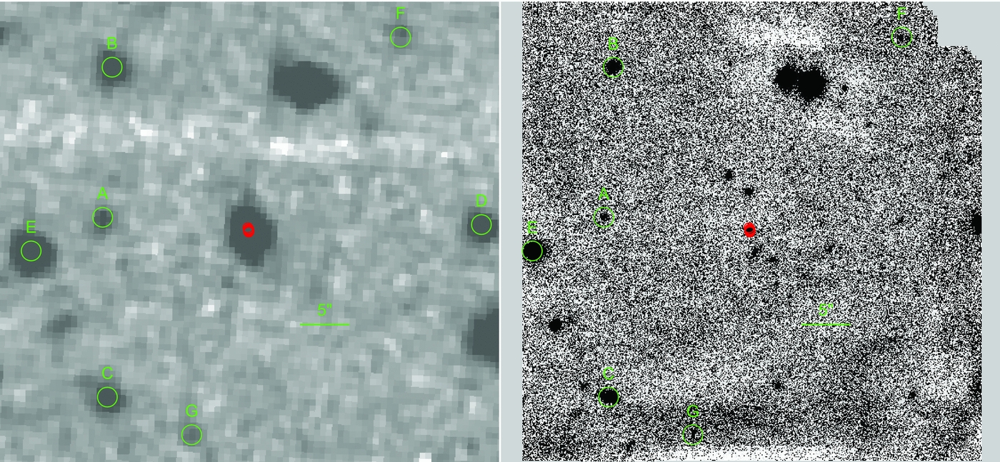
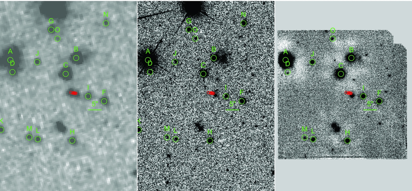
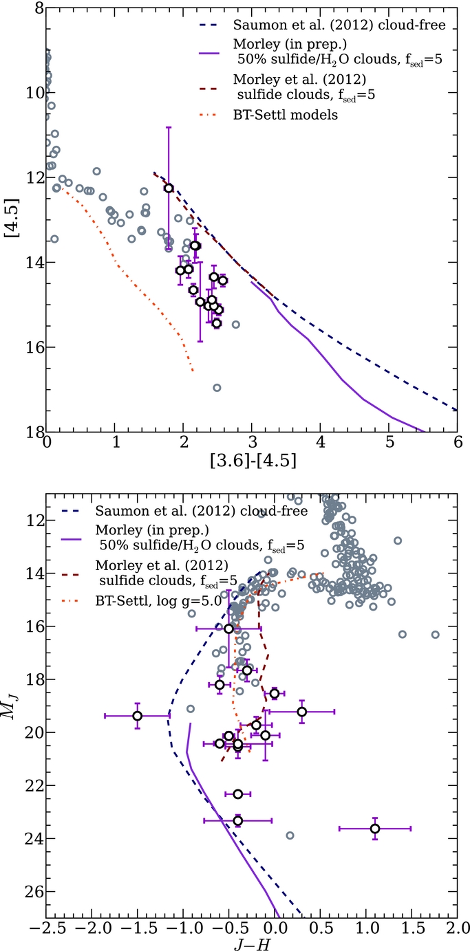
There are numerous reasons why both molecular cloud fragmentation and disk fragmentation produce fewer brown dwarfs than stars. While the opacity-limited minimum mass of fragments (either disk-born or cloud-born) is only 1–10 MJup (Low & Lynden-Bell 1976; Larson 2005; Whitworth & Stamatellos 2006), such fragments typically accrete mass and become stars (Bate et al. 2003; Kratter et al. 2010) given typical masses for molecular cloud cores and onset times for protostellar collapse (Myers 2009). Vorobyov (2013) argues that the probability of fragment survival in gravitationally unstable disks is low, as inward migration and subsequent ejection of fragments is efficient. Vorobyov also shows that fragment survival requires that the instability must happen in the T-Tauri phase of disk evolution, rather than the embedded phase, yet the necessary conditions for T-Tauri disk fragmentation may occur only rarely. The median disk/star mass ratio of Class II YSOs inferred from dust continuum observations is only 0.9% (Andrews & Williams 2005, 2007). Even when gas is observed directly, as in the deuterated H2 (HD) observations of TW Hydrae (Bergin et al. 2013), the masses inferred are almost always less than the 0.1Mdisk/M* threshold required for disk fragmentation (Rafikov 2005).
If molecular cloud formation and disk fragmentation are both unlikely, it makes sense to consider whether core accretion—the planet formation process in which a solid core eventually grows large enough to hydrodynamically accrete gas from a disk—might form low-mass field brown dwarfs. Numerical simulations by Ford et al. (2001) show that 30% of the interactions between two giant planets near the stability boundary result in ejection, while microlensing measurements by Sumi et al. (2011) reveal a population of possibly unbound 1 MJup planetary-mass objects in the galactic bulge. Mordasini et al. (2012) find that the planet mass produced by core accretion falls off dramatically for M > 3 MJup in disks with M < 0.06 M☉, which would explain the dearth of high-mass planets and field brown dwarfs. Yet Veras & Raymond (2012) argue that planet–planet scattering alone cannot explain the large number of unbound planets discovered by Sumi et al., who estimate two free-floating planets per solar-type star. Veras & Raymond instead suggest that other mechanisms for forming free floaters must be at work.
The likely formation mechanism for the free-floating objects presented here depends sensitively on their mass and velocity dispersion. In most cases the masses inferred from the BT-Settl and Morley models are consistent with either disk fragmentation or star-like formation, as most of the objects are above the rolloff in the planetary-mass function predicted by Mordasini et al. (2012). For the lowest mass Y dwarfs, such as WISE 1828+2650 (∼5–10 MJup), core accretion followed by ejection from a planetary system might be the more favored mechanism as such low-mass objects are at or below the opacity-limited minimum mass. However, core accretion near the star (where formation of a massive planet is favorable) followed by planet–planet scattering produces objects with a high velocity dispersion. Our objects have tangential velocities consistent with stars in the solar neighborhood and inconsistent with an origin in nearby young clusters (i.e., <100 pc and <100 Myr (Section 5.2)), implying that core accretion and ejection from a close-packed planetary system is unlikely. Both star-like formation and disk fragmentation followed by the ejection of partially contracted clumps (Basu & Vorobyov 2012) produce objects with low velocity dispersion, as observed for young brown dwarfs in Cha I (Joergens & Guenther 2001). Distinguishing between star-like formation and disk instability is difficult, as both mechanisms are consistent with the observed IMF (Hennebelle & Chabrier 2009; Stamatellos & Whitworth 2009). In a review of brown dwarf observations to date, Luhman et al. (2007) conclude that star-like formation is the most likely origin for low-mass free floaters, whereas Bate (2012) argues that star-like formation, disk fragmentation, and ejection of collapsing cores from molecular clouds probably operate together. The existence of mass solutions that are typical for star-like formation or disk fragmentation, combined with the low velocity dispersion, suggests that our objects are brown dwarfs rather than free-floating planets.
6. CONCLUSIONS
We have carried out a program of imaging a selection of the coldest brown dwarfs detected by the WISE satellite, including six late T and nine Y dwarfs to obtain multi-epoch astrometry over a 2 to 3 yr baseline. From these data we have determined parallax and proper motions with better than 15% accuracy for most of the sample, with well-determined distances ranging from 6 to 14 pc. By comparing absolute [4.5] mag and a variety of colors from our Keck, HST, and Spitzer photometry with models for low-mass objects, we can estimate masses and ages for this sample ranging between 3.4–8.8 Gyr and 12–30 MJup for the best-fitting BT-Settl models. The fits for the coldest objects (e.g., WISE 1828+2650) are quite poor, so these values remain highly uncertain. On the modeling side there is an urgent need for Y dwarf models with a broad range of metallicity, non-equilibrium chemistry, and effective temperatures as low as 300 K. Highly optically thick dust clouds (AV > 10 mag) may be required to suppress the short wavelength emission and improve the agreement with the models. Observationally, it is critical to anchor these models with a few T or Y dwarf binaries for which dynamical masses can be obtained. In the future, long wavelength photometry out to >10 μm with JWST will provide model-independent bolometric luminosities and effective temperatures. Moderate resolution spectroscopy from 1 to 10 μm will provide diagnostic spectral lines that can give much more precise information on physical conditions, especially surface gravity, than can broadband photometry.
Our parallaxes are similar to those estimated by other authors and confirm that local population of coldest brown dwarfs is sparse. The relative lack of brown dwarfs with masses below ∼15 MJup or exoplanets with masses above 10 MJup suggest that this is a difficult mass range for the formation of objects in either environment. The dispersion in tangential velocities for our objects suggest that the objects detected by WISE are, however, likely to represent the lowest mass end of the star formation process, rather than a population of objects formed by core accretion in a protoplanetary disk that we subsequently ejected (at high velocity) from their parent system.
The research described in this publication was carried out in part at the Jet Propulsion Laboratory, California Institute of Technology, under a contract with the National Aeronautics and Space Administration (NASA). This publication makes use of data products from the Wide-field Infrared Survey Explorer, which is a joint project of the University of California, Los Angeles, and the Jet Propulsion Laboratory/California Institute of Technology, funded by NASA. This research has made use of the NASA/IPAC Infrared Science Archive (IRSA) and the NASA Exoplanet Archive, which are operated by the Jet Propulsion Laboratory, California Institute of Technology, under contract with NASA. This work is based in part on observations made with the Spitzer Space Telescope, which is operated by the Jet Propulsion Laboratory, California Institute of Technology, under a contract with NASA. This work is also based in part on observations made with the NASA/ESA Hubble Space Telescope, obtained at the Space Telescope Science Institute, which is operated by the Association of Universities for Research in Astronomy, Inc., under NASA contract NAS 5-26555. These observations are associated with program 12330. Support for program #12330 was provided by NASA through a grant from the Space Telescope Science Institute. Some data presented herein were obtained at the W. M. Keck Observatory from telescope time allocated to NASA through the agency's scientific partnership with the California Institute of Technology and the University of California. The Observatory was made possible by the generous financial support of the W. M. Keck Foundation. The authors recognize and acknowledge the very significant cultural role and reverence that the summit of Mauna Kea has always had within the indigenous Hawaiian community. We are most fortunate to have the opportunity to conduct observations from this mountain. The 2MASS catalog and RECONS database of nearby stars remain invaluable resources. We acknowledge the assistance of Tahina Ramiaramanantsoa with the early stages of the reduction of these data and Dimitra Touli with the model fitting. Finally, we thank the anonymous referee for a careful reading of our paper, which led to a number of valuable improvements to both its content and presentation.
Footnotes
- 9
The Spitzer colors and absolute magnitude suggest a Y dwarf classification, but no confirming spectrum has yet been obtained.
- 10
All the photometric measurements reported herein were made using this routine from the IDL ASTRO library, http://idlastro.gsfc.nasa.gov/contents.html. A number of other IDL routines are also taken from this library.
- 11
- 12
The post-BCD images have 0
6 pixels derived from the 122 native pixel data. The aperture correction is described in http://irsa.ipac.caltech.edu/data/SPITZER/docs/irac. - 13
- 14
- 15
- 16
Argus/IC2391, TW Hydrae, Tucana/Horologium, β Pictoris, AB Doradus, hCha, Cha-near, Columba, and the Hyades. See Beichman et al. (2013).