


ABSTRACT
We present the results of a multiplicity survey of 91 stars spanning masses of ∼0.2–10 M☉ in the Upper Scorpius star-forming region, based on adaptive optics imaging with the Gemini North telescope. Our observations identified 29 binaries, 5 triples, and no higher order multiples. The corresponding raw multiplicity frequency is 0.37 ± 0.05. In the regime where our observations are complete—companion separations of 0 1–5'' (∼15–800 AU) with magnitude limits ranging from K < 9.3 at 01 to K < 15.8 at 5''—the multiplicity frequency is 0.27
 . For similar separations, the multiplicity frequency in Upper Scorpius is comparable to that in other dispersed star-forming regions, but is a factor of two to three higher than in denser star-forming regions or in the field. Our sample displays a constant multiplicity frequency as a function of stellar mass. Among our sample of binaries, we find that both wider (>100 AU) and higher-mass systems tend to have companions with lower companion-to-primary mass ratios. Three of the companions identified in our survey are unambiguously substellar and have estimated masses below 0.04 M☉ (two of them are new discoveries from this survey—1RXS J160929.1−210524b and HIP 78530B—although we have reported them separately in earlier papers). These three companions have projected orbital separations of 300–900 AU. Based on a statistical analysis factoring in sensitivity limits, we calculate an occurrence rate of 5–40 MJup companions of ∼4.0% for orbital separations of 250–1000 AU, compared to <1.8% at smaller separations, suggesting that such companions are more frequent on wider orbits.
Export citation and abstract BibTeX RIS
1. INTRODUCTION
The star formation process has been a subject of great interest in astrophysics for a long time, and several aspects are still not understood in great detail. Nowadays, after the discoveries of hundreds of brown dwarfs and planets—both as companions to stars and as free floating objects—this fundamental question has widened in scope to include the origins of brown dwarfs and giant planets as well. Indeed, the formation processes of these different classes of objects, spanning over three orders of magnitudes in mass, are strongly coupled together. Several different mechanisms are likely involved in their formation, and a given process can likely form objects of different classes. This is particularly true for multiple systems. For example, stellar companions could form through the direct fragmentation of a collapsing prestellar core (e.g., Goodwin et al. 2004a; Delgado-Donate et al. 2004; Bate 2012) or through the collapse of a massive circumstellar disk (e.g., Kratter et al. 2010a), and both of these processes could also result in the formation of brown dwarf companions, or even planets (e.g., Boss 2011; Kratter et al. 2010b). The various processes involved have varying efficiencies in different regimes of orbital separations, companion mass ratios, or stellar masses and would thus leave distinct imprints on the multiplicity properties of a given population of stars. The level of turbulence in the initial molecular cloud and prestellar cores is also likely to play a significant role in star formation and can influence the fraction of stars found in multiple systems, as well as the degree of high-order multiplicity (e.g., Goodwin et al. 2004b). Similarly, the star density of the birth environment can alter the properties of multiple systems through dynamical effects (e.g., Kroupa et al. 2001; Parker et al. 2009). A good characterization of the multiplicity properties of stellar systems is thus an important diagnostic of the origins of stars, brown dwarfs, and massive planets. To enable a good and detailed comparison with theoretical modeling of the various processes, this should be achieved across the entire ranges of orbital separations, primary star masses, and companion masses, and for different ages and different environments.
Based on various observational approaches (e.g., radial velocity, adaptive optics imaging, astrometry), several studies have been made over the past two decades to characterize the properties of multiple stars. These studies targeted stars in the field (e.g., Duquennoy & Mayor 1991; Fischer & Marcy 1992; Raghavan et al. 2010; Janson et al. 2012), in young open clusters or stellar associations (e.g., Patience et al. 2002; Chauvin et al. 2002; Brandeker et al. 2003), and in star-forming regions (e.g., Ghez et al. 1997; Kohler & Leinert 1998; Kraus et al. 2006; Kouwenhoven et al. 2007a). For a good global review of the properties of multiple systems, the reader is directed to Duchêne & Kraus (2013). Other useful reviews, somewhat more focused in scope, are presented in Duchêne et al. (2007), Goodwin et al. (2007), and Burgasser et al. (2007). While significant progress has been made, the overall picture of stellar multiplicity remains incomplete (see Duchêne & Kraus 2013) and more studies would be useful, namely, to increase the sample sizes, extend the orbital separation ranges probed, and lower the companion mass detection limits in a more uniform manner for the different samples.
In this paper, we present the results of an adaptive optics (AO) multiplicity survey of 91 stars with masses of ∼0.2 M☉ to ∼10 M☉ in the young Upper Scorpius (US) star-forming region (∼5 Myr, ∼145 pc, Preibisch et al. 2002). The US association is part of the larger Scorpius–Centaurus (Sco-Cen) complex, which also includes Upper Centaurus Lupus (UCL) and Lower Centaurus Crux (LCC). These three subgroups have different ages—US being the youngest one—and are close but well separated on the sky, which makes identification of their members straightforward. This complex is thus particularly good to study star formation as it provides distinct stellar populations born from a similar environment but at different ages. The age of the US association has traditionally been taken to be 5 Myr (e.g., Preibisch et al. 2002), with a very small age spread among its members (±1 Myr). This age has been recently put into question by Pecaut et al. (2012) based on isochrone fitting in an H-R diagram; these authors instead suggest an age of ∼11 Myr for US and ages of ∼16 Myr and ∼17 Myr for UCL and LCC, respectively. However, the model-independent analysis of Song et al. (2012), based on the lithium line strengths of G, K, and M stars in Sco-Cen compared to those of stars in the young TW Hydrae (∼8 Myr) and β Pictoris (∼12 Myr) associations, indicates that UCL and LCC are both younger than β Pictoris, and thus likely aged ∼10 Myr. So given that US is known to be younger than UCL and LCC, the initial age estimate of 5 Myr for US appears reasonable, and this is what we will adopt in this paper when age is needed.
In addition to the survey presented here, we previously completed a similar study of the Chamaeleon I (∼1–2 Myr) star-forming region (Lafrenière et al. 2008a; also see Ahmic et al. 2007), we have recently completed a study of the intermediate-mass stars of the larger Sco-Cen complex (Janson et al. 2013), and we are currently completing a study for the Taurus star-forming region (∼1 Myr; S. Daemgen et al., in preparation). These studies have comparable sensitivities in terms of contrast and angular resolution and together span stellar ages of ∼1–10 Myr.
2. TARGET SELECTION, OBSERVATIONS, AND DATA REDUCTION
The target sample was selected from the list of 218 US members with Spitzer observations that were studied by Carpenter et al. (2006, 2009) to investigate the presence of circumstellar disks. The original Carpenter et al. sample was built from a thorough literature compilation of US members, where membership was assessed based on astrometry, H-R diagram position, Li abundance, and X-ray emission, to which they applied further cuts to ensure a high membership probability (e.g., on proper motions and distances) and a good photometric quality. Thus, this sample should not be biased for or against multiplicity, or for or against the presence of circumstellar disks.5 We chose the Carpenter et al. sample to build our target list as the Spitzer observations and the results of Carpenter et al. (2006, 2009) offer the added possibility of investigating the connection between the presence of companions and circumstellar disks. As one goal of the current work is to study how the multiplicity properties vary as a function of mass, we built a list of 105 targets by randomly selecting roughly equal numbers of stars in logarithmically spaced mass bins spanning 0.1 to ∼10 M☉. The method used to estimate the masses of the target stars is detailed in Section 3.4. We obtained observations for 91 stars in our list; their basic properties are given in Table 1. The 14 stars of our initial list of 105 that were not observed were all later than M3 and all required the use of the laser guide star (LGS; see below); they were not observed due to inadequate observing conditions for LGS operation. The direct effect is that we observed relatively few targets below 0.3 M☉ and only one target below 0.2 M☉, limiting our statistics in these regimes. Also, as these stars were removed from our sample based, effectively, on their faintness (need for LGS), we cannot exclude that this has preferentially removed single stars from our sample at the lowest primary masses (≲ 0.25 M☉), and thus slightly overestimated the fraction of multiples in this regime. This is difficult to quantify but, in any case, would have little impact on the conclusions of this paper.
Table 1. Target Properties
| Name | R.A. | Decl. | Ks | Spectral | Teffa | Massb |
|---|---|---|---|---|---|---|
| (J2000.0) | (J2000.0) | (mag) | Typea | (K) | (M☉) | |
| HIP 81266 | 16 35 52.96 | −28 12 57.7 | 3.70 | B0V | 30000 | 16. |
| HIP 78265 | 15 58 51.11 | −26 06 50.7 | 3.69 | B1V+B2V | 25400 | 10. |
| HIP 78933 | 16 06 48.43 | −20 40 08.8 | 4.01 | B1V | 25400 | 10. |
| HIP 77635 | 15 50 58.75 | −25 45 04.6 | 4.78 | B1.5Vn | 23700 | 9.0 |
| HIP 77859 | 15 53 55.87 | −23 58 41.0 | 5.36 | B2V | 22000 | 7.8 |
| HIP 78104 | 15 56 53.07 | −29 12 50.8 | 4.46 | B2IV/V | 22000 | 7.8 |
| HIP 79374 | 16 11 59.74 | −19 27 38.1 | 3.88 | B2IV | 22000 | 7.8 |
| HIP 79404 | 16 12 18.21 | −27 55 35.0 | 4.98 | B2V | 22000 | 7.8 |
| HIP 77840 | 15 53 36.70 | −25 19 37.9 | 4.79 | B2.5Vn | 20350 | 6.8 |
| HIP 78168 | 15 57 40.46 | −20 58 59.2 | 5.73 | B3V | 18700 | 5.9 |
| HIP 77858 | 15 53 53.92 | −24 31 59.2 | 5.36 | B5V | 15400 | 4.2 |
| HIP 78246 | 15 58 34.87 | −24 49 53.2 | 5.65 | B5V | 15400 | 4.2 |
| HIP 79530 | 16 13 45.49 | −24 25 19.6 | 6.08 | B6IV | 14000 | 3.7 |
| HIP 77900 | 15 54 30.11 | −27 20 19.1 | 6.30 | B7V | 13000 | 3.3 |
| HIP 78207 | 15 58 11.36 | −14 16 45.5 | 4.59 | B8Ia/Iab | 11900 | 2.9 |
| HIP 76633 | 15 39 00.06 | −19 43 56.9 | 7.49 | B9V | 10500 | 2.5 |
| HIP 78530 | 16 01 55.47 | −21 58 49.6 | 6.90 | B9V | 10500 | 2.5 |
| HIP 78702 | 16 04 00.24 | −19 46 02.9 | 7.24 | B9V | 10500 | 2.5 |
| HIP 78549 | 16 02 13.56 | −22 41 14.9 | 6.97 | B9.5V | 10010 | 2.4 |
| HIP 78956 | 16 07 04.68 | −16 56 35.7 | 7.22 | B9.5V | 10010 | 2.4 |
| HIP 76310 | 15 35 16.10 | −25 44 03.1 | 7.17 | A0V | 9520 | 2.4 |
| HIP 78196 | 15 57 59.35 | −31 43 44.2 | 7.03 | A0V | 9520 | 2.4 |
| HIP 78847 | 16 05 43.39 | −21 50 19.6 | 7.14 | A0V | 9520 | 2.4 |
| HIP 79124 | 16 09 02.61 | −18 59 44.0 | 7.01 | A0V | 9520 | 2.4 |
| HIP 79156 | 16 09 20.89 | −19 27 25.9 | 7.48 | A0V | 9520 | 2.4 |
| HIP 80311 | 16 23 47.17 | −26 16 15.8 | 7.97 | A0V | 9520 | 2.4 |
| HIP 79250 | 16 10 25.35 | −23 06 23.4 | 7.24 | A3III/IV | 8720 | 2.3 |
| HIP 77457 | 15 48 52.13 | −29 29 00.2 | 7.28 | A7IV | 7850 | 2.2 |
| HIP 80059 | 16 20 28.13 | −21 30 32.4 | 7.50 | A7III/IV | 7850 | 2.2 |
| HIP 79643 | 16 15 09.27 | −23 45 34.8 | 8.03 | F2 | 6890 | 2.1 |
| HIP 82319 | 16 49 12.21 | −22 42 41.7 | 7.88 | F3V | 6740 | 2.1 |
| HIP 78483 | 16 01 18.42 | −26 52 21.3 | 7.55 | G0V | 6030 | 2.0 |
| 1RXS J155500.0−234729 | 15 54 59.86 | −23 47 18.2 | 7.03 | G3V | 5830 | 1.9 |
| 1RXS J161949.6−335456 | 16 19 50.58 | −33 54 45.4 | 8.41 | G3 | 5830 | 1.9 |
| 1RXS J155820.3−183725 | 15 58 20.55 | −18 37 25.2 | 7.61 | G4 | 5800 | 1.9 |
| 1RXS J154106.9−265643 | 15 41 06.79 | −26 56 26.3 | 8.92 | G7 | 5630 | 1.8 |
| 1RXS J154131.4−252043 | 15 41 31.22 | −25 20 36.3 | 7.24 | G8e | 5520 | 1.7 |
| 1RXS J161318.0−221251 | 16 13 18.59 | −22 12 48.9 | 7.43 | G9 | 5410 | 1.7 |
| 1RXS J160126.1−224047 | 16 01 25.64 | −22 40 40.3 | 8.52 | K1IV | 5080 | 1.4 |
| 1RXS J161329.9−231122 | 16 13 29.29 | −23 11 07.5 | 8.49 | K1 | 5080 | 1.4 |
| 1RXS J160446.5−193031 | 16 04 47.76 | −19 30 23.1 | 8.04 | K2IV | 4900 | 1.2 |
| RX J1604.3−2130 | 16 04 21.66 | −21 30 28.4 | 8.51 | K2 | 4900 | 1.2 |
| 1RXS J160814.2−190845 | 16 08 14.74 | −19 08 32.8 | 8.43 | K2 | 4900 | 1.2 |
| 1RXS J153557.0−232417 | 15 35 57.80 | −23 24 04.6 | 9.43 | K3: | 4730 | 1.0 |
| 1RXS J155848.4−175758 | 15 58 47.73 | −17 57 59.5 | 8.32 | K3 | 4730 | 1.0 |
| 1RXS J160251.5−240204 | 16 02 51.24 | −24 01 57.4 | 8.93 | K4 | 4590 | 0.95 |
| 1RXS J161303.8−225745 | 16 13 02.72 | −22 57 44.6 | 8.45 | K4 | 4590 | 0.95 |
| 1RXS J160210.1−224128 | 16 02 10.45 | −22 41 28.0 | 8.06 | K5IV | 4350 | 0.84 |
| 1RXS J161121.6−182119 | 16 11 20.58 | −18 20 54.9 | 8.56 | K5IV | 4350 | 0.84 |
| [PZ99] J160357.6−203105 | 16 03 57.68 | −20 31 05.5 | 8.37 | K5 | 4350 | 0.84 |
| 1RXS J160612.4−203655 | 16 06 12.54 | −20 36 47.2 | 8.90 | K5 | 4350 | 0.84 |
| [PZ99] J160856.7−203346 | 16 08 56.73 | −20 33 46.0 | 8.62 | K5 | 4350 | 0.84 |
| RX J1614.3−1906 | 16 14 20.30 | −19 06 48.1 | 7.81 | K5 | 4350 | 0.84 |
| [PGZ2001] J160643.8−190805 | 16 06 43.86 | −19 08 05.6 | 9.19 | K6 | 4205 | 0.77 |
| 1RXS J160042.0−212730 | 16 00 42.77 | −21 27 38.0 | 8.92 | K7 | 4060 | 0.71 |
| 1RXS J160239.3−254157 | 16 02 39.11 | −25 42 07.9 | 9.12 | K7 | 4060 | 0.71 |
| 1RXS J160929.1−210524 | 16 09 30.30 | −21 04 58.9 | 8.92 | K7 | 4060 | 0.71 |
| [PGZ2001] J161031.9−191305 | 16 10 31.96 | −19 13 06.2 | 8.99 | K7 | 4060 | 0.71 |
| 1RXS J160801.7−202755 | 16 08 01.42 | −20 27 41.7 | 9.29 | K8 | 3990 | 0.68 |
| 1RXS J155405.2−292032 | 15 54 03.58 | −29 20 15.4 | 8.73 | M0 | 3850 | 0.61 |
| [PZ99] J155716.6−252918 | 15 57 16.74 | −25 29 19.3 | 8.86 | M0 | 3850 | 0.61 |
| 1RXS J155748.8−230521 | 15 57 50.03 | −23 05 09.4 | 9.27 | M0 | 3850 | 0.61 |
| 1RXS J160108.6−211320 | 16 01 08.01 | −21 13 18.5 | 8.80 | M0 | 3850 | 0.61 |
| 1RXS J160355.8−203138 | 16 03 54.96 | −20 31 38.4 | 8.62 | M0 | 3850 | 0.61 |
| 1RXS J160831.4−180253 | 16 08 31.38 | −18 02 41.4 | 8.90 | M0 | 3850 | 0.61 |
| 1RXS J160621.5−192851 | 16 06 21.96 | −19 28 44.6 | 8.62 | M0.5V | 3777 | 0.56 |
| RX J155734.4−232112 | 15 57 34.31 | −23 21 12.3 | 8.99 | M1V | 3705 | 0.51 |
| 1RXS J154413.0−252307 | 15 44 13.34 | −25 22 59.1 | 9.08 | M1 | 3705 | 0.51 |
| 1RXS J160200.7−222133 | 16 02 00.39 | −22 21 23.7 | 8.84 | M1 | 3705 | 0.51 |
| 1RXS J160703.4−191138 | 16 07 03.94 | −19 11 33.9 | 9.22 | M1 | 3705 | 0.51 |
| [PGZ2001] J160823.8−193551 | 16 08 23.88 | −19 35 51.8 | 9.25 | M1 | 3705 | 0.51 |
| [PGZ2001] J160954.4−190654 | 16 09 54.41 | −19 06 55.1 | 9.60 | M1 | 3705 | 0.51 |
| [PGZ2001] J161115.3−175721 | 16 11 15.34 | −17 57 21.4 | 9.20 | M1 | 3705 | 0.51 |
| RX J155629.3−234821 | 15 56 29.42 | −23 48 19.8 | 8.74 | M1.5V | 3632 | 0.43 |
| 1RXS J160542.2−200413 | 16 05 42.67 | −20 04 15.0 | 9.16 | M2V | 3560 | 0.37 |
| [PGZ2001] J160341.8−200557 | 16 03 41.87 | −20 05 57.8 | 9.49 | M2 | 3560 | 0.37 |
| [PGZ2001] J160502.1−203507 | 16 05 02.14 | −20 35 07.0 | 9.45 | M2 | 3560 | 0.37 |
| [PGZ2001] J160545.4−202308 | 16 05 45.40 | −20 23 08.8 | 10.41 | M2 | 3560 | 0.37 |
| [PGZ2001] J160707.7−192715 | 16 07 07.67 | −19 27 16.1 | 9.80 | M2 | 3560 | 0.37 |
| [PGZ2001] J160739.4−191747 | 16 07 39.40 | −19 17 47.2 | 9.80 | M2 | 3560 | 0.37 |
| [PGZ2001] J160823.5−191131 | 16 08 23.57 | −19 11 31.6 | 9.93 | M2 | 3560 | 0.37 |
| [PGZ2001] J160933.8−190456 | 16 09 33.78 | −19 04 56.2 | 9.85 | M2 | 3560 | 0.37 |
| [PGZ2001] J160222.4−195653 | 16 02 22.49 | −19 56 53.8 | 10.66 | M3 | 3415 | 0.28 |
| [PGZ2001] J160428.4−190441 | 16 04 28.39 | −19 04 41.4 | 9.28 | M3 | 3415 | 0.28 |
| 1RXS J160652.6−241627 | 16 06 54.36 | −24 16 10.8 | 8.86 | M3 | 3415 | 0.28 |
| [PBB2002] USco J161052.4−193734 | 16 10 52.41 | −19 37 34.4 | 10.73 | M3 | 3415 | 0.28 |
| [PBB2002] USco J155918.4−221042 | 15 59 18.39 | −22 10 43.1 | 10.07 | M4 | 3270 | 0.22 |
| [PGZ2001] J160801.5−192757 | 16 08 01.57 | −19 27 57.9 | 9.69 | M4 | 3270 | 0.22 |
| [PGZ2001] J160959.4−180009 | 16 09 59.33 | −18 00 09.1 | 10.34 | M4 | 3270 | 0.22 |
| [PGZ2001] J161118.1−175728 | 16 11 18.13 | −17 57 28.7 | 9.33 | M4 | 3270 | 0.22 |
| [PBB2002] USco J161011.0−194603 | 16 10 11.01 | −19 46 04.1 | 11.38 | M5 | 3125 | 0.18 |
Notes. aFrom Carpenter et al. (2006). bEstimate based on Teff and the models of D'Antona & Mazzitelli (1997) and Schaller et al. (1992); see text for more detail.
The observations were obtained with the NIRI camera (Hodapp et al. 2003) and the ALTAIR AO system (Herriot et al. 2000) at the Gemini North Telescope (program GN-2008A-Q-45). For all observations, the field lens of ALTAIR was used to reduce off-axis Strehl degradation due to anisoplanatism, and the f/32 camera of NIRI was used for a pixel size of 21.4 mas6 and a field of view of 219 × 219. All observations were made in the K band using the Ks, K', or  filter. For all targets, we used a five-point dither pattern corresponding to the center and four corners of a square of side 10''. At each dither position, we obtained one co-addition of several short integrations in fast, high read-noise mode, and one ∼10 s integration in slow, low read-noise mode. At each position, this provides an unsaturated image of the target star and a much deeper image of the field that can be spatially registered and scaled in flux without ambiguity. For targets fainter than R ∼ 13.5 the LGS was used for wave front sensing and the target itself was used for tip/tilt guiding; in these cases, only non-saturated images were obtained as the targets are fainter. To use a shorter exposure time and avoid saturation for the very brightest targets (K < 5), only a 512 × 512 sub-array of the detector was read and the dither square was reduced to 5'' on a side. In those cases, larger offsets were made after the observation of the target to acquire sky frames. All observations were obtained with the instrument rotator turned off to maximize the correlation between the stellar point-spread function (PSF) of different targets, such that the images of different targets could be used for PSF subtraction or fitting if desired. A log of the observations is given in Table 2, along with information on the image quality and the detection limits achieved.
Table 2. Observations Log
| Name | UT Date | Filter | texp (s) | FWHM | Strehl | Detection Limits (K mag) | ||||||
|---|---|---|---|---|---|---|---|---|---|---|---|---|
| Unsat. | Sat. | (mas) | Ratio | 01 |
025 |
05 |
1'' | 2'' | 5'' | |||
| HIP 81266a | 2008 Jun 10 |  |
30 | 60 | 91 | 0.20 | 7.2 | 9.5 | 10.8 | 12.9 | 14.7 | 17.0 |
| HIP 78265a | 2008 May 21 |  |
26 | 60 | ⋅⋅⋅ | ⋅⋅⋅ | 6.8 | 9.3 | 10.8 | 13.0 | 14.4 | 16.8 |
| HIP 78933a | 2008 May 22 |  |
30 | 60 | 83 | 0.28 | 7.7 | 10.3 | 11.7 | 13.9 | 15.3 | 17.6 |
| HIP 77635a | 2008 May 21 |  |
30 | 60 | 77 | 0.32 | 8.8 | 11.3 | 12.4 | 14.7 | 16.2 | 18.3 |
| HIP 77859 | 2008 May 21 |  |
30 | 50 | 77 | 0.32 | 9.3 | 11.7 | 13.1 | 15.3 | 16.7 | 18.9 |
| HIP 78104a | 2008 May 21 |  |
26 | 60 | 77 | 0.32 | 8.4 | 11.0 | 12.2 | 14.4 | 15.9 | 18.1 |
| HIP 79374a | 2008 May 21 |  |
30 | 60 | ⋅⋅⋅ | ⋅⋅⋅ | 6.1 | 9.3 | 10.7 | 12.2 | 13.4 | 15.9 |
| HIP 79404a | 2008 May 22 |  |
30 | 60 | 81 | 0.24 | 8.7 | 11.2 | 12.4 | 14.5 | 16.3 | 18.1 |
| HIP 77840a | 2008 May 21 |  |
30 | 60 | 74 | 0.35 | 8.2 | 10.6 | 11.9 | 14.0 | 15.2 | 17.5 |
| HIP 78168 | 2008 May 21 |  |
30 | 50 | 76 | 0.31 | 9.6 | 12.1 | 13.5 | 15.7 | 17.2 | 19.1 |
| HIP 77858 | 2008 May 21 |  |
27 | 50 | 79 | 0.30 | 9.2 | 11.8 | 13.0 | 15.3 | 16.7 | 18.9 |
| HIP 78246 | 2008 May 22 |  |
30 | 50 | 79 | 0.31 | 9.6 | 12.0 | 13.5 | 15.5 | 17.1 | 19.1 |
| HIP 79530 | 2008 May 22 |  |
30 | 50 | 77 | 0.32 | 9.3 | 11.7 | 13.2 | 15.1 | 16.5 | 18.3 |
| HIP 77900 | 2008 May 21 |  |
24 | 50 | 76 | 0.32 | 10.2 | 12.8 | 14.1 | 16.3 | 17.7 | 19.3 |
| HIP 78207a | 2008 May 26 |  |
30 | 60 | 78 | 0.33 | 8.5 | 11.1 | 12.3 | 14.6 | 16.0 | 18.1 |
| HIP 76633 | 2008 May 21 |  |
30 | 50 | 75 | 0.34 | 11.5 | 14.0 | 15.4 | 17.6 | 18.9 | 19.5 |
| HIP 78530 | 2008 May 24 |  |
30 | 50 | 75 | 0.35 | 10.2 | 12.7 | 14.0 | 16.1 | 17.6 | 18.7 |
| HIP 78702 | 2008 May 25 |  |
30 | 50 | 79 | 0.29 | 11.2 | 13.6 | 15.1 | 17.1 | 18.5 | 19.4 |
| HIP 78549 | 2008 Jun 10 |  |
30 | 50 | 69 | 0.35 | 10.4 | 12.5 | 13.9 | 16.2 | 17.8 | 18.8 |
| HIP 78956 | 2008 May 4 |  |
30 | 50 | 73 | 0.31 | 10.6 | 12.9 | 14.0 | 15.7 | 17.6 | 18.5 |
| HIP 76310 | 2008 May 21 |  |
24 | 50 | 76 | 0.34 | 11.1 | 13.7 | 15.0 | 17.2 | 18.6 | 19.5 |
| HIP 78196 | 2008 May 21 |  |
24 | 50 | 76 | 0.32 | 11.1 | 13.4 | 14.8 | 17.1 | 18.5 | 19.4 |
| HIP 78847 | 2008 May 27 |  |
30 | 50 | 77 | 0.32 | 10.2 | 12.8 | 14.2 | 16.3 | 17.8 | 18.6 |
| HIP 79124 | 2008 May 25 |  |
30 | 50 | 82 | 0.30 | 10.2 | 12.6 | 14.0 | 16.0 | 17.6 | 18.6 |
| HIP 79156 | 2008 May 4 |  |
30 | 50 | 72 | 0.29 | 10.9 | 12.9 | 14.3 | 16.3 | 18.1 | 18.7 |
| HIP 80311 | 2008 Jun 10 |  |
30 | 50 | 71 | 0.31 | 12.0 | 14.3 | 15.6 | 17.7 | 19.1 | 19.5 |
| HIP 79250 | 2008 May 4 |  |
30 | 50 | 74 | 0.31 | 10.7 | 12.7 | 14.1 | 16.2 | 17.9 | 18.6 |
| HIP 77457 | 2008 May 21 |  |
30 | 50 | 76 | 0.32 | 11.2 | 13.8 | 15.0 | 17.3 | 18.7 | 19.5 |
| HIP 80059 | 2008 May 4 |  |
30 | 50 | 71 | 0.30 | 10.9 | 12.8 | 14.2 | 16.3 | 18.0 | 18.6 |
| HIP 79643 | 2008 Jun 10 | Ks | 30 | 50 | 76 | 0.31 | 11.3 | 13.6 | 14.9 | 17.0 | 18.8 | 20.1 |
| HIP 82319 | 2008 May 4 |  |
30 | 50 | 71 | 0.31 | 11.3 | 13.4 | 14.8 | 16.8 | 18.4 | 18.8 |
| HIP 78483 | 2008 Jun 10 |  |
30 | 50 | 71 | 0.34 | 10.8 | 12.7 | 14.3 | 16.4 | 18.1 | 18.7 |
| 1RXS J155500.0−234729 | 2008 May 4 |  |
30 | 50 | 74 | 0.29 | 10.4 | 12.6 | 13.6 | 15.7 | 17.5 | 18.5 |
| 1RXS J161949.6−335456 | 2008 May 26 | Ks | 30 | 50 | 79 | 0.29 | 12.2 | 14.6 | 16.1 | 18.2 | 20.0 | 20.9 |
| 1RXS J155820.3−183725 | 2008 May 4 |  |
30 | 50 | 71 | 0.31 | 11.1 | 13.2 | 14.5 | 16.6 | 18.2 | 18.8 |
| 1RXS J154106.9−265643 | 2008 May 21 | Ks | 30 | 50 | 76 | 0.35 | 12.4 | 14.8 | 16.1 | 18.3 | 19.9 | 20.4 |
| 1RXS J154131.4−252043 | 2008 May 21 |  |
27 | 50 | 76 | 0.32 | 11.0 | 13.7 | 15.1 | 17.3 | 18.7 | 19.5 |
| 1RXS J161318.0−221251 | 2008 May 4 |  |
30 | 50 | 71 | 0.32 | 11.6 | 13.8 | 15.2 | 17.3 | 18.8 | 19.5 |
| 1RXS J160126.1−224047 | 2008 May 2 | Ks | 30 | 50 | 76 | 0.20 | 12.2 | 14.2 | 15.4 | 17.4 | 19.5 | 20.5 |
| 1RXS J161329.9−231122 | 2008 May 2 | Ks | 30 | 50 | 82 | 0.12 | 10.8 | 12.8 | 13.9 | 15.8 | 17.9 | 19.2 |
| 1RXS J160446.5−193031 | 2008 Mar 22 | Ks | 30 | 50 | 84 | 0.22 | 11.8 | 13.9 | 15.2 | 17.2 | 19.2 | 20.8 |
| RX J1604.3−2130 | 2008 Mar 23 | Ks | 30 | 50 | 87 | 0.12 | 11.7 | 13.5 | 14.6 | 16.5 | 18.7 | 20.3 |
| 1RXS J160814.2−190845 | 2008 Mar 22 | Ks | 30 | 50 | 79 | 0.23 | 12.3 | 14.3 | 15.6 | 17.5 | 19.5 | 20.9 |
| 1RXS J153557.0−232417 | 2008 Mar 23 | Ks | 32 | 50 | 86 | 0.15 | 12.8 | 14.7 | 15.9 | 17.9 | 20.0 | 20.6 |
| 1RXS J155848.4−175758 | 2008 Mar 23 | Ks | 30 | 50 | 78 | 0.20 | 12.0 | 14.0 | 15.2 | 17.2 | 19.3 | 20.7 |
| 1RXS J160251.5−240204 | 2008 Mar 23 | Ks | 30 | 50 | 77 | 0.21 | 12.1 | 14.0 | 15.2 | 17.2 | 19.3 | 20.2 |
| 1RXS J161303.8−225745 | 2008 Mar 23 | Ks | 30 | 50 | 78 | 0.22 | 11.5 | 13.5 | 14.8 | 16.8 | 18.9 | 20.2 |
| 1RXS J160210.1−224128 | 2008 Mar 23 | Ks | 30 | 50 | 77 | 0.23 | 11.0 | 12.4 | 13.7 | 15.9 | 17.9 | 18.7 |
| 1RXS J161121.6−182119 | 2008 Apr 1 | Ks | 30 | 50 | 97 | 0.10 | 11.5 | 13.4 | 14.5 | 16.5 | 18.6 | 20.0 |
| [PZ99] J160357.6−203105 | 2008 Mar 23 | Ks | 30 | 50 | 81 | 0.21 | 12.1 | 14.1 | 15.4 | 17.4 | 19.4 | 20.9 |
| 1RXS J160612.4−203655 | 2008 Apr 7 | Ks | 30 | 50 | 85 | 0.15 | 12.4 | 14.2 | 15.4 | 17.4 | 19.5 | 20.6 |
| [PZ99] J160856.7−203346 | 2008 Mar 25 | Ks | 30 | 50 | 77 | 0.32 | 12.8 | 14.9 | 16.3 | 18.5 | 20.3 | 21.3 |
| RX J1614.3−1906 | 2008 Apr 7 |  |
30 | 50 | 94 | 0.11 | 10.9 | 12.7 | 14.0 | 16.0 | 18.0 | 18.3 |
| [PGZ2001] J160643.8−190805 | 2008 Apr 7 | Ks | 30 | 50 | 83 | 0.22 | 12.1 | 13.8 | 15.4 | 17.5 | 19.5 | 20.1 |
| 1RXS J160042.0−212730 | 2008 Apr 7 | Ks | 30 | 50 | 85 | 0.19 | 12.5 | 14.5 | 15.8 | 17.8 | 19.8 | 20.6 |
| 1RXS J160239.3−254157 | 2008 Apr 7 | Ks | 36 | 50 | 85 | 0.15 | 12.5 | 14.5 | 15.7 | 17.6 | 19.7 | 20.6 |
| 1RXS J160929.1−210524 | 2008 Apr 27 | Ks | 30 | 50 | 71 | 0.29 | 12.4 | 14.2 | 15.6 | 17.5 | 19.6 | 20.4 |
| [PGZ2001] J161031.9−191305 | 2008 Apr 21 | Ks | 30 | 50 | 89 | 0.12 | 11.3 | 13.2 | 14.4 | 16.3 | 18.5 | 19.4 |
| 1RXS J160801.7−202755 | 2008 Mar 28 | Ks | 32 | 50 | 84 | 0.25 | 12.8 | 15.2 | 16.8 | 18.9 | 20.7 | 21.1 |
| 1RXS J155405.2−292032 | 2008 Apr 7 | Ks | 30 | 50 | 94 | 0.12 | 11.1 | 12.9 | 14.2 | 16.2 | 18.2 | 19.1 |
| [PZ99] J155716.6−252918 | 2008 Apr 18 | Ks | 30 | 50 | 82 | 0.22 | 11.6 | 13.6 | 14.4 | 16.2 | 18.3 | 19.3 |
| 1RXS J155748.8−230521 | 2008 Apr 18 | Ks | 32 | 50 | 90 | 0.19 | 12.6 | 14.9 | 16.2 | 18.3 | 20.3 | 20.6 |
| 1RXS J160108.6−211320 | 2008 Apr 26 | Ks | 30 | 50 | 75 | 0.22 | 12.6 | 14.6 | 15.7 | 17.8 | 19.8 | 20.7 |
| 1RXS J160355.8−203138 | 2008 Apr 27 | Ks | 30 | 50 | ⋅⋅⋅ | ⋅⋅⋅ | 11.3 | 13.5 | 15.0 | 17.0 | 19.0 | 19.9 |
| 1RXS J160831.4−180253 | 2008 Apr 3 | Ks | 30 | 50 | 89 | 0.11 | 12.0 | 13.7 | 15.0 | 17.0 | 19.2 | 20.3 |
| 1RXS J160621.5−192851b | 2008 May 29 | Ks | 30 | 50 | 104 | 0.14 | 10.2 | 12.8 | 13.7 | 15.6 | 17.8 | 18.8 |
| RX J155734.4−232112 | 2008 Apr 18 | Ks | 30 | 50 | 95 | 0.19 | 11.3 | 14.0 | 15.3 | 17.5 | 19.4 | 19.9 |
| 1RXS J154413.0−252307 | 2008 Apr 18 | Ks | 32 | 50 | 90 | 0.21 | 12.4 | 14.9 | 16.3 | 18.4 | 20.3 | 20.7 |
| 1RXS J160200.7−222133 | 2008 May 2 | Ks | 30 | 50 | 84 | 0.13 | 12.0 | 13.9 | 15.1 | 17.0 | 19.2 | 19.9 |
| 1RXS J160703.4−191138 | 2008 Apr 26 | Ks | 32 | 50 | 82 | 0.16 | 11.9 | 13.8 | 15.0 | 17.0 | 18.9 | 19.4 |
| [PGZ2001] J160823.8−193551 | 2008 Apr 3 | Ks | 32 | 50 | 100 | 0.07 | 11.1 | 12.5 | 14.0 | 16.0 | 17.8 | 18.7 |
| [PGZ2001] J160954.4−190654 | 2008 Apr 26 | Ks | 32 | 50 | 83 | 0.17 | 13.0 | 15.0 | 16.3 | 18.4 | 20.3 | 20.4 |
| [PGZ2001] J161115.3−175721 | 2008 Apr 16 | Ks | 32 | 50 | 117 | 0.05 | 11.4 | 12.8 | 14.2 | 16.4 | 18.5 | 19.2 |
| RX J155629.3−234821 | 2008 Apr 18 | Ks | 30 | 50 | 88 | 0.21 | 10.8 | 12.9 | 14.2 | 16.5 | 18.4 | 19.1 |
| 1RXS J160542.2−200413 | 2008 Apr 27 | Ks | 32 | 50 | 80 | 0.25 | 12.2 | 14.2 | 15.1 | 17.0 | 18.9 | 19.7 |
| [PGZ2001] J160341.8−200557 | 2008 Apr 27 | Ks | 32 | 50 | 80 | 0.24 | 13.3 | 15.4 | 16.8 | 18.9 | 20.7 | 21.0 |
| [PGZ2001] J160502.1−203507b | 2008 May 26 | Ks | 75 | ⋅⋅⋅ | 102 | 0.13 | 11.5 | 14.3 | 16.1 | 18.4 | 19.0 | 19.0 |
| [PGZ2001] J160545.4−202308b | 2008 Aug 15 | K' | 80 | ⋅⋅⋅ | 88 | 0.15 | 12.7 | 15.1 | 16.0 | 18.1 | 18.6 | 18.6 |
| [PGZ2001] J160707.7−192715b | 2008 Jun 19 | Ks | 75 | ⋅⋅⋅ | 91 | 0.10 | 12.4 | 14.3 | 15.6 | 17.7 | 18.4 | 18.4 |
| [PGZ2001] J160739.4−191747b | 2008 Jun 26 | Ks | 75 | ⋅⋅⋅ | 96 | 0.11 | 12.3 | 14.8 | 15.9 | 17.9 | 18.8 | 18.8 |
| [PGZ2001] J160823.5−191131b | 2008 May 25 | Ks | 75 | ⋅⋅⋅ | 90 | 0.17 | 13.0 | 15.4 | 16.5 | 18.4 | 19.1 | 19.1 |
| [PGZ2001] J160933.8−190456b | 2008 Aug 17 | K' | 75 | ⋅⋅⋅ | 87 | 0.17 | 13.0 | 15.2 | 16.7 | 18.8 | 19.3 | 19.3 |
| [PGZ2001] J160222.4−195653b | 2008 Aug 15 | K' | 80 | ⋅⋅⋅ | 88 | 0.16 | 13.7 | 15.9 | 17.1 | 19.0 | 19.4 | 19.4 |
| [PGZ2001] J160428.4−190441 | 2008 May 26 | Ks | 32 | 50 | 98 | 0.14 | 10.6 | 13.3 | 15.3 | 17.2 | 18.5 | 18.8 |
| 1RXS J160652.6−241627 | 2008 Apr 27 | Ks | 30 | 50 | 72 | 0.33 | 12.4 | 14.3 | 15.7 | 17.7 | 19.0 | 20.0 |
| [PBB2002] USco J161052.4−193734b | 2008 Aug 15 | K' | 80 | ⋅⋅⋅ | 100 | 0.11 | 13.3 | 15.8 | 17.0 | 18.6 | 18.9 | 19.0 |
| [PBB2002] USco J155918.4−221042b | 2008 Aug 19 | K' | 80 | ⋅⋅⋅ | 136 | 0.04 | 12.1 | 13.7 | 14.7 | 16.6 | 17.8 | 17.8 |
| [PGZ2001] J160801.5−192757b | 2008 Jun 26 | Ks | 75 | ⋅⋅⋅ | 162 | 0.03 | 10.7 | 12.3 | 13.3 | 14.5 | 15.6 | 15.8 |
| [PGZ2001] J160959.4−180009b | 2008 Jun 22 | Ks | 80 | ⋅⋅⋅ | 89 | 0.15 | 13.3 | 15.7 | 16.8 | 18.7 | 19.3 | 19.4 |
| [PGZ2001] J161118.1−175728b | 2008 Jun 24 | Ks | 75 | ⋅⋅⋅ | ⋅⋅⋅ | ⋅⋅⋅ | 9.8 | 11.5 | 13.2 | 15.6 | 16.4 | 16.4 |
| [PBB2002] USco J161011.0−194603b | 2008 May 27 | Ks | 90 | ⋅⋅⋅ | 102 | 0.14 | 14.2 | 16.7 | 17.8 | 19.5 | 19.9 | 19.9 |
| Follow-up | ||||||||||||
| HIP 78104c | 2010 Jul 6 |  |
72 | 360 | 74 | 0.27 | ⋅⋅⋅ | ⋅⋅⋅ | ⋅⋅⋅ | ⋅⋅⋅ | ⋅⋅⋅ | ⋅⋅⋅ |
| HIP 79374a | 2010 Apr 27 |  |
15 | 45 | ⋅⋅⋅ | ⋅⋅⋅ | ⋅⋅⋅ | ⋅⋅⋅ | ⋅⋅⋅ | ⋅⋅⋅ | ⋅⋅⋅ | ⋅⋅⋅ |
| HIP 78847 | 2010 Jul 3 |  |
100 | 75 | ⋅⋅⋅ | ⋅⋅⋅ | ⋅⋅⋅ | ⋅⋅⋅ | ⋅⋅⋅ | ⋅⋅⋅ | ⋅⋅⋅ | ⋅⋅⋅ |
| HIP 79250a | 2010 Apr 27 | K' | 30 | 100 | 78 | 0.25 | ⋅⋅⋅ | ⋅⋅⋅ | ⋅⋅⋅ | ⋅⋅⋅ | ⋅⋅⋅ | ⋅⋅⋅ |
| HIP 82319a | 2008 Jun 17 | H | 24 | 50 | 69 | 0.19 | ⋅⋅⋅ | ⋅⋅⋅ | ⋅⋅⋅ | ⋅⋅⋅ | ⋅⋅⋅ | ⋅⋅⋅ |
| HIP 82319a | 2008 Jun 17 | J | 24 | 50 | 67 | 0.08 | ⋅⋅⋅ | ⋅⋅⋅ | ⋅⋅⋅ | ⋅⋅⋅ | ⋅⋅⋅ | ⋅⋅⋅ |
| 1RXS J155500.0−234729 | 2010 Jul 4 |  |
80 | ⋅⋅⋅ | 78 | 0.30 | ⋅⋅⋅ | ⋅⋅⋅ | ⋅⋅⋅ | ⋅⋅⋅ | ⋅⋅⋅ | ⋅⋅⋅ |
| 1RXS J161949.6−335456a | 2010 Jun 29 | K' | 84 | ⋅⋅⋅ | 80 | 0.28 | ⋅⋅⋅ | ⋅⋅⋅ | ⋅⋅⋅ | ⋅⋅⋅ | ⋅⋅⋅ | ⋅⋅⋅ |
| 1RXS J155820.3−183725a | 2010 Feb 21 | K' | 83 | ⋅⋅⋅ | 80 | 0.29 | ⋅⋅⋅ | ⋅⋅⋅ | ⋅⋅⋅ | ⋅⋅⋅ | ⋅⋅⋅ | ⋅⋅⋅ |
| 1RXS J155820.3−183725a | 2010 Jul 6 | K' | 83 | ⋅⋅⋅ | 80 | 0.29 | ⋅⋅⋅ | ⋅⋅⋅ | ⋅⋅⋅ | ⋅⋅⋅ | ⋅⋅⋅ | ⋅⋅⋅ |
| 1RXS J154106.9−265643 | 2010 Jun 16 | K' | 120 | ⋅⋅⋅ | 85 | 0.25 | ⋅⋅⋅ | ⋅⋅⋅ | ⋅⋅⋅ | ⋅⋅⋅ | ⋅⋅⋅ | ⋅⋅⋅ |
| 1RXS J154106.9−265643 | 2010 Jul 4 | K' | 120 | 50 | 79 | 0.27 | ⋅⋅⋅ | ⋅⋅⋅ | ⋅⋅⋅ | ⋅⋅⋅ | ⋅⋅⋅ | ⋅⋅⋅ |
| 1RXS J160251.5−240204 | 2010 Jul 4 | K' | 50 | 50 | 79 | 0.25 | ⋅⋅⋅ | ⋅⋅⋅ | ⋅⋅⋅ | ⋅⋅⋅ | ⋅⋅⋅ | ⋅⋅⋅ |
| 1RXS J161303.8−225745 | 2010 Jun 18 | K' | 56 | 70 | 82 | 0.23 | ⋅⋅⋅ | ⋅⋅⋅ | ⋅⋅⋅ | ⋅⋅⋅ | ⋅⋅⋅ | ⋅⋅⋅ |
| [PGZ2001] J161031.9−191305 | 2010 Jun 18 | K' | 80 | ⋅⋅⋅ | ⋅⋅⋅ | ⋅⋅⋅ | ⋅⋅⋅ | ⋅⋅⋅ | ⋅⋅⋅ | ⋅⋅⋅ | ⋅⋅⋅ | ⋅⋅⋅ |
| [PGZ2001] J161031.9−191305 | 2010 Jul 3 | K' | 80 | 50 | ⋅⋅⋅ | ⋅⋅⋅ | ⋅⋅⋅ | ⋅⋅⋅ | ⋅⋅⋅ | ⋅⋅⋅ | ⋅⋅⋅ | ⋅⋅⋅ |
| [PGZ2001] J161031.9−191305 | 2010 Jul 23 | K' | 80 | 50 | ⋅⋅⋅ | ⋅⋅⋅ | ⋅⋅⋅ | ⋅⋅⋅ | ⋅⋅⋅ | ⋅⋅⋅ | ⋅⋅⋅ | ⋅⋅⋅ |
| [PGZ2001] J161031.9−191305 | 2010 Jul 23 | H | 90 | ⋅⋅⋅ | ⋅⋅⋅ | ⋅⋅⋅ | ⋅⋅⋅ | ⋅⋅⋅ | ⋅⋅⋅ | ⋅⋅⋅ | ⋅⋅⋅ | ⋅⋅⋅ |
| [PGZ2001] J161031.9−191305 | 2010 Jul 23 | J | 90 | ⋅⋅⋅ | ⋅⋅⋅ | ⋅⋅⋅ | ⋅⋅⋅ | ⋅⋅⋅ | ⋅⋅⋅ | ⋅⋅⋅ | ⋅⋅⋅ | ⋅⋅⋅ |
| 1RXS J155405.2−292032 | 2010 Jun 16 | K' | 100 | ⋅⋅⋅ | 92 | 0.20 | ⋅⋅⋅ | ⋅⋅⋅ | ⋅⋅⋅ | ⋅⋅⋅ | ⋅⋅⋅ | ⋅⋅⋅ |
| 1RXS J160355.8−203138 | 2010 Jul 6 | K' | 56 | 105 | ⋅⋅⋅ | ⋅⋅⋅ | ⋅⋅⋅ | ⋅⋅⋅ | ⋅⋅⋅ | ⋅⋅⋅ | ⋅⋅⋅ | ⋅⋅⋅ |
| [PGZ2001] J160222.4−195653 | 2010 Feb 22 | K' | 112 | ⋅⋅⋅ | 103 | 0.14 | ⋅⋅⋅ | ⋅⋅⋅ | ⋅⋅⋅ | ⋅⋅⋅ | ⋅⋅⋅ | ⋅⋅⋅ |
| [PGZ2001] J160222.4−195653 | 2010 Jul 2 | K' | 128 | ⋅⋅⋅ | 127 | 0.04 | ⋅⋅⋅ | ⋅⋅⋅ | ⋅⋅⋅ | ⋅⋅⋅ | ⋅⋅⋅ | ⋅⋅⋅ |
Notes. aOnly a 512 × 512 subarray of the detector was read. bObservations made with the laser guide star. cObservations made in Angular Differential Imaging mode.
The data were reduced using custom IDL routines. A sky frame was constructed by taking the median of the images at all dither positions after masking out the regions dominated by the target's signal. The sky images acquired off target were simply median-combined without masking. After subtraction of this sky frame, the images were divided by a normalized flat field. Then isolated bad pixels were replaced by the interpolated value of a third-order polynomial surface fit to the good pixels in a 7 × 7 pixel box, while clustered bad pixels were simply masked out. Next, the images were distortion corrected using the distortion solution provided by the Gemini staff.7 Finally, the long-exposure images were properly scaled in intensity and merged with their corresponding short-exposure images, and the resulting images were co-aligned and co-added. All reduced images were also individually saved for further measurements.
An initial analysis of the images revealed the presence of several interesting candidate companions whose true association with the target stars was difficult to assess based on the limited data available; see Sections 3.1 and 3.2. We followed up a few of those targets quickly after the initial detection in other filters to measure their colors and help assess their nature, but for most systems we obtained follow-up K-band imaging with Altair/NIRI two years later to check whether the candidate companions are co-moving with the primary (program GN-2010A-Q-18). A summary of the follow-up observations is given in Table 2. The follow-up observations of the 1RXS J160929.1−210524 and HIP 78530 systems, which were both found and confirmed to harbor low-mass substellar companions, are omitted from the table as they are reported elsewhere (Lafrenière et al. 2008b, 2010, 2011) and are not discussed here. The observing strategy for the follow-up observations was the same as above except that the instrument rotator was turned on. This was done to simplify the observations and reduce the overhead time during acquisition, but as a result the field-of-view orientation on the chip was significantly different compared to the first epoch observations and, given the important distortion residuals, this significantly reduced our astrometric precision and complicated the common proper motion analysis. This is discussed further in Section 3.3. The data reduction was done as explained above.
3. ANALYSIS
3.1. Identification of Companions
We visually inspected the images to identify all point sources, which include obvious components of multiple systems and several fainter candidate companions. Then, depending on their separation and relative brightness, we computed the position and flux of the detected sources relative to the primary stars using one or more of the three following methods. For the first method, we determined the centroid by fitting a 2D Gaussian+Moffat function and the flux ratio using aperture photometry. For the second, used for well-separated and relatively bright sources, we found the relative position and flux by minimizing the residual noise after subtraction of one component from another. For the third, used for the tightest systems, we determined the parameters by fitting a reference PSF image, taken from a single target star observed shortly before or after the target considered. Whenever possible, we compared the results from different methods and always found them to be consistent with each other. When the sources were clearly detected in the individual images, we made the measurements in the individual images and averaged them together; otherwise, we made the measurements on the averaged image only. We used the dispersion among the individual measurements or the difference between measurements made using two different methods to estimate the measurement errors; these errors are typically very small (a few mas) but can be important for the faintest sources (∼10 mas). The overall error appears to be dominated by systematic geometric distortion residuals, as noted earlier for similar observations (e.g., Lafrenière et al. 2010). A total of 190 companions or candidate companions were identified around the 91 target stars; their separation and contrast are shown in Figure 1, and their measurements are given in Table 3. The (candidate) companions detected span a range of separations from ∼005 up to ∼10'' (i.e., ∼7–1500 AU), although our observations are only mostly complete in the 01–5'' separation range (i.e., ∼15–700 AU); see Section 3.5 for more details on our survey sensitivity and completeness.

Figure 1. All companions (diamonds) and background stars (small triangles) identified around our target stars. The dashed lines indicate the contrast limits reached for at least 90% (top curve) and 50% (bottom curve) of our targets. The two companions near ΔK of 7 are 1RXS J160929.1−210524b (left) and HIP 78530B (right), which we previously published separately.
Download figure:
Standard image High-resolution imageTable 3. Sources Detected Around Target Stars
| Name | Separationa | P.A.a | ΔK | Edetb | Ndetc | Statusd |
|---|---|---|---|---|---|---|
| ('') | (deg) | (mag) | ||||
| HIP 78104 | 2.680 ± 0.005 | 0.52 ± 0.09 | 10.19 ± 0.14 | 0.53 | 2 | B1 |
| HIP 79374e | 0.072 ± 0.001 | 346.35 ± 0.20 | 1.65 ± 0.03 | 4.4 × 10⁻⁷ | 0 | C0 |
| ⋅⋅⋅ | 1.351 ± 0.001 | 1.80 ± 0.01 | 0.69 ± 0.02 | 7.9 × 10⁻⁵ | 0 | C0 |
| ⋅⋅⋅ | 5.323 ± 0.001 | 318.04 ± 0.01 | 10.14 ± 0.10 | 1.6 | 3 | B1 |
| HIP 77840 | 2.061 ± 0.001 | 268.28 ± 0.02 | 1.89 ± 0.02 | 0.00088 | 0 | C0 |
Notes.
aOnly the measurement errors are given. There is an additional systematic uncertainty in separation of 15 mas for <4'', 25 mas for <8'', and 50 mas for <12'', as well as a systematic uncertainty of 0 15 in P.A. These uncertainties apply to comparison with measurements made with other instruments, and to comparison between the two epochs presented here.
bFor the observations of our 91 target stars, this is the expected total number of detected background sources of the same brightness or brighter and within the same angular separation. See text for more detail.
cActual number of such background sources detected by our survey.
dStatus of candidate companion: (C0) bound companion based on statistical arguments (and sometimes known from other work); (C1) bound companion based on follow-up from this work; (C2) bound companion based on other work; (B0) background based on statistical arguments; (B1) background based on follow-up from this work; (B2) background based on other work; (?) undetermined. See Sections 3.2 and 3.3 for more detail.
eMeasurements given are from our follow-up epoch, 2010 April 27.
fWhen the same source appears on multiple lines, the corresponding epochs are in the order given in Table 2.
gMeasurements given are from our first epoch, 2008 May 21.
15 in P.A. These uncertainties apply to comparison with measurements made with other instruments, and to comparison between the two epochs presented here.
bFor the observations of our 91 target stars, this is the expected total number of detected background sources of the same brightness or brighter and within the same angular separation. See text for more detail.
cActual number of such background sources detected by our survey.
dStatus of candidate companion: (C0) bound companion based on statistical arguments (and sometimes known from other work); (C1) bound companion based on follow-up from this work; (C2) bound companion based on other work; (B0) background based on statistical arguments; (B1) background based on follow-up from this work; (B2) background based on other work; (?) undetermined. See Sections 3.2 and 3.3 for more detail.
eMeasurements given are from our follow-up epoch, 2010 April 27.
fWhen the same source appears on multiple lines, the corresponding epochs are in the order given in Table 2.
gMeasurements given are from our first epoch, 2008 May 21.
Only a portion of this table is shown here to demonstrate its form and content. A machine-readable version of the full table is available.
Download table as: DataTypeset image
Upon visual inspection, a few of the sources identified appeared to be potentially marginally (un)resolved binaries and were examined more closely. This is the case of the secondary of the HIP 79643 system: it is clearly elongated compared with the other sources in the field of view (including the primary). We thus treat it as a tight binary, and we used a PSF template (that of the primary star) to fit for its separation and contrast. Despite relatively poor AO correction resulting in an elongated PSF, the PSF of the primary star HIP 79374 appears to be significantly more elongated than that of its secondary companion at 134. As there was an interesting wide candidate companion around this star, it was observed again in our follow-up program, and the second-epoch data, of much better quality, clearly confirm the tight binary nature of the primary star, making this a triple system. The PSF of the tertiary component was used as a template to fit the tight binary and determine its parameters. Given the better image quality, the second-epoch measurements are given in the tables. 1RXS J155405.2−29203A is also elongated relative to its secondary companion at 143 and subtraction of the latter from the former leaves significant residuals. This source could thus be itself a tight binary, but the data at hand are insufficient to determine this with confidence. The PSF of RX J155734.4−232112 is significantly elongated relative to the faint point source 46 away, consistent with it being a marginally unresolved binary. This star was resolved into a binary by Kraus et al. (2008) using aperture masking interferometry. We thus treat this star as a binary and use a PSF template (different star observed on same night) to fit for its separation and contrast; our measurements are consistent with those reported by Kraus et al. (2008). The four tightest (marginally resolved) binaries identified in our survey are shown in Figure 2; all the other binaries were clearly resolved.
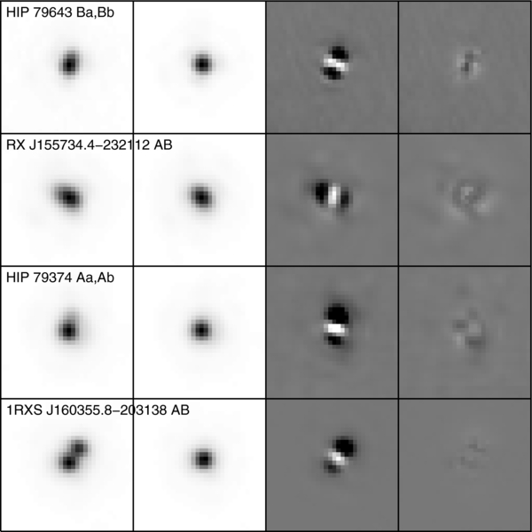
Figure 2. Four tightest binaries identified in our survey. From left to right, the columns, respectively, show the image of the binary, the image of the corresponding PSF, the residual image after subtraction of a single-component fit, and the residual image after subtraction of a two-component fit. The intensity scale is linear, and the intensity range is the same for both residual images of a given row. Each panel has a size 068; north is up, and east is to the left. Except for RX J155734.4−232112 AB, all PSF templates are from another star present in the same image as the binary; for RX J155734.4−232112 AB, the PSF template is from a different star observed on the same night using the same instrument settings.
Download figure:
Standard image High-resolution image3.2. Probability of Chance Alignment
We used star counts based on the Two Micron All-Sky Survey (2MASS) Point Source Catalog (PSC) to assess the likelihood that the numerous candidate companions identified in our images are unrelated background stars rather than real companions; a similar approach was used by Correia et al. (2006), and we used the same approach in Lafrenière et al. (2008a) for our survey of Chamaeleon I. For each target in our sample, we first retrieved all sources from the 2MASS PSC that lie within a radius of 15' and built a logarithmic cumulative distribution of the number of sources as a function of Ks magnitude. A straight line can fit these distributions extremely well from Ks ∼ 7 up to the 2MASS completeness limit of Ks ∼ 15, and thus these distributions can reasonably be extrapolated linearly to fainter magnitudes when needed; we have indeed done so for Ks = 15–20.8 We next converted the logarithmic cumulative distributions to surface densities as a function of limiting magnitude. Then based on these curves, we calculated, for each of the 190 sources identified, the probability that a background star at least as bright and within the same angular separation would have been found and detected around each of the 91 targets in our survey. Finally, for each candidate companion, by summing these background source detection probabilities over the 91 target stars, we obtained Edet, the expected total number of background sources of the same brightness or brighter and within the same angular separation as the candidate companion that should have been detected by our survey. The value of Edet is indicative of the likelihood of each candidate companion being truly bound or an unrelated background source: candidates with higher values are more likely to be a background source. As a validity check for our approach, for each candidate we have also counted the number of sources with the same characteristics that were actually detected in our survey, Ndet; these numbers should be close to Edet if the background source surface densities that we used are correct. As shown in Table 3, Ndet and Edet are always of the same order, confirming the legitimacy of our approach.
The sources identified and listed in Table 3 generally fall into two main categories, having either Edet ≪ 1 or Edet ≫ 1 (this is also visible in Figure 1 in the form of a dearth of detected sources with 4 < ΔK < 7). In all likelihood, the former are truly bound companions and the latter are unrelated background stars. For the purpose of this paper, we considered those sources with Edet ⩽ 0.05 as bound, since, according to Poisson statistics, the probability that they are indeed bound is ⩾95%. On the other hand, we considered candidates with Edet ⩾ 3 to be background, again assuming Poisson statistics, as the probability that they are indeed background is ⩾95%. There are 22 sources with an ambiguous status (around 19 stars), having 0.05 < Edet < 3. These include 1RXS J160929.1−210524b and HIP 78530B, both of which we have already followed up and confirmed to be real companions (Lafrenière et al. 2008b, 2010, 2011). Of the 17 other sources, 16 have been observed through our follow-up programs and are discussed in the next subsection (only [PGZ2001] J160545.4−202308 was not re-observed). The properties of all multiple systems—those with probabilities ⩾95% of being bound or those confirmed to be through follow-up—are given in Table 5.
3.3. Verification of Ambiguous Candidates
For the ambiguous candidates with follow-up astrometric observations, we compared the measured relative positions of the candidate sources at the different epochs to determine, based on the known proper motion of the primary star, whether they are co-moving with their primary or unrelated background stars. When not available from the revised Hipparcos catalog (van Leeuwen 2007), the proper motions of the stars were taken from the UCAC3 catalog (Zacharias et al. 2010). As mentioned above, our follow-up observations suffered from systematic astrometric errors due to significant distortion residuals combined with largely different field-of-view orientations between the initial and follow-up observations. We assessed the magnitude of this systematic uncertainty using background sources detected in our data at the two epochs and found it to be 15 mas for separations <4'', 25 mas for <8'', and 50 mas for <12''. The systematic uncertainty in position angle is 015. Despite these uncertainties, valid conclusions could be made for the majority of the candidates followed up.
For most candidates (27 from HIP 78104, 53 from HIP 79374, 29 from 1RXS J161949.6−335456, 16 and 124 from 1RXS J161303.8−225745, 33 from 1RXSJ155405.2−292032, 28 and 43 from 1RXS J160355.8−203138, and 53 from [PGZ2001] J160222.4−195653), the relative measurements are in much better agreement with the changes expected for a distant stationary background star; these candidates are thus treated as unrelated stars. For three candidates, however, the measurements are consistent with common proper motion; these are the bright source 89 from HIP 78847, the source 58 from [PGZ2001] J161031.9−191305, and the source 63 from 1RXS J154106.9−265643. Note that the latter two companions were previously detected and considered to be bound companions by Kraus et al. (2008) and Kraus & Hillenbrand (2009).
For the remaining candidates with astrometric follow-up (30 from HIP 79250, 111 from 1RXS J155500.0−234729, 56 from 1RXS J155820.3−183725, and 723 from 1RXS J160251.5−240204), our measurements do not allow us to reach a definitive conclusion because of the significant systematic astrometric errors noted earlier. Of those, the object around 1RXS J155500.0−234729 was confirmed to be a background source by Metchev & Hillenbrand (2009), while the object around 1RXS J160251.5−240204 is indicated to be a known companion in Kraus et al. (2008); the remaining two objects are treated as unrelated for the purpose of this paper. Finally, the candidate 27 from HIP 82319, which was followed up with photometry only, has colors of an early star (J − K = 0.25, H − K = 0.0) and is thus considered to be a background source.
3.4. Mass Estimates
The masses of all targets were estimated from their estimated effective temperature and the predictions of pre-main-sequence evolution models for an age of 5 Myr. This approach is less affected by unresolved binarity, uncertainties in extinction (although small in US), or uncertainties in distance and was thus preferred over a determination based on the source luminosity. To be able to estimate masses in a consistent manner across most of the range of masses observed, we primarily used the models of D'Antona & Mazzitelli (1997),9 which cover the mass range 0.017–3 M☉, sufficient for all but the 14 most massive stars in our sample. For these 14 stars, we used the models from Schaller et al. (1992), which are in excellent agreement with those of D'Antona & Mazzitelli (1997) at 2–3 M☉, where the transition is made. This combination of models enables determination of the masses of all primary stars observed and all but the lowest mass companion found (1RXS J160929.1−210524b). The estimated masses of all targets are indicated in Table 1.
The mass ratios of the secondary (and tertiary) components of multiple systems were estimated based on their K-band contrast with respect to their primary. More precisely, the observed K-band contrast of the companion was added to the model K-band absolute magnitude of the primary (i.e., derived from the models based on its effective temperature), and the corresponding companion mass was then obtained from the models; this approach was preferred because contrast is not affected by uncertainties in distance and—to first order—extinction. For reference, the model K-band magnitude versus mass (or effective temperature) relation used here is shown in Figure 3. The estimated absolute magnitude of 1RXS J160929.1−210524b falls beyond the faint limit of the evolution models of D'Antona & Mazzitelli (1997), so for this companion we simply used the mass estimated in Lafrenière et al. (2008b).
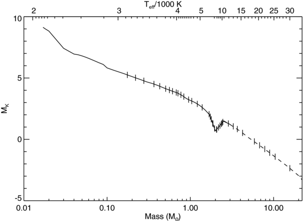
Figure 3. Absolute K-band magnitude as a function of mass from the models of D'Antona & Mazzitelli (1997, solid line) and of Schaller et al. (1992, dashed line), for an age of 5 Myr. The upper axis shows the corresponding effective temperatures according to the models. The vertical ticks on the curve mark the masses of the primary stars targeted in this study.
Download figure:
Standard image High-resolution imageFor all mass estimates we have assumed a fixed age of 5 Myr, but we note that an uncertainty on the age of ±1 Myr would typically translate into an uncertainty on the masses of ±2% for <0.5 M☉, ±4% for 0.5–1.5 M☉ and ±7% for 1.5–3 M☉, with a smaller effect on the inferred mass ratios.10 The uncertainties on the primary stars' effective temperature also affect our mass estimates. Assuming a typical uncertainty of ±0.5 subtype for the classification of the primaries leads to typical uncertainties on the temperatures of ±2% for <10,000 K and ±6% for hotter stars. In turn, this leads to uncertainties on the derived masses of ±5%–10% for <10 M☉ and up to ±20% for higher masses. On top of these uncertainties, one must also consider the uncertainties in the models themselves. These can be quite large. For example, using the models of Baraffe et al. (1998) would lead to masses higher by 25%–50% depending on the effective temperature of the star and the mixing length parameter value used for the models. The effect on the mass ratios is somewhat lower, with differences of 10%–30% between the two models. The actual mass and mass ratio values quoted in this work thus bear large uncertainties and must be used with care, but as shown in Lafrenière et al. (2008a), these uncertainties and the particular choice of models should not significantly affect the main conclusions of this paper. The caveats mentioned above should also be kept in mind when comparing our results with those of other surveys, for which the methodology and models used for the mass estimates could be different.
3.5. Detection Limits
The detection limits as a function of angular separation from the target stars were obtained by calculating the standard deviation of the residual signal in annuli centered on the target after subtraction of an azimuthally symmetric PSF profile. The detection limits were determined as five times this standard deviation. For multiple systems, the secondary and/or tertiary component were subtracted from the image using an analytic or template PSF model prior to the calculation of the detection limits. Since at the smallest separations the variance of the residual noise may be underestimated by this procedure as there are too few independent spatial elements within the corresponding annuli, we have required that the detection limits within a radius of 2 FWHM be no better than the PSF intensity profile. Mass ratio limits have also been calculated for each target based on their K-band contrast limits using the approach described above, with the only difference here being that, as the contrast limits reached often corresponded to masses below the lowest mass of the models of D'Antona & Mazzitelli 1997 (0.017 M☉), we extended the models below 0.017 M☉ using the models with DUSTY atmospheres from Baraffe et al. (2003) and Chabrier et al. (2000). Both sets of models agree very well around the transition point (within 0.017–0.04 M☉).
The K-band detection limits achieved for each individual target are indicated in Table 2 for six angular separations ranging from 01 to 5'' (∼15–700 AU). They are also summarized, along with contrast and mass ratio limits, in Table 4. The table reports the detection limits achieved simultaneously throughout the 01''−05 range for at least 50% and 90% of the stars in our sample; the latter limits can be viewed as a completeness limit for our sample. In brief, the contrast limits achieved for at least 90% of the sample are 4.1 mag at 025, 7.1 mag at 1'', and 7.5 mag at 5''; the corresponding mass ratio limits are 0.063, 0.017, and 0.015, respectively. Finally, as the limits achieved bear some dependence on the primary star mass (or more specifically on the star brightness), Table 4 also presents the limits corresponding to different primary mass bins. For instance, the contrast limits are not as good for fainter targets and targets observed with LGS due to poorer AO correction, and a brighter apparent magnitude limit was reached for brighter targets in both the contrast- and background-limited regimes, the latter case being due to the use of a narrowband filter.
Table 4. Sample Detection Limits
| Mass Bin | Separation | |||||
|---|---|---|---|---|---|---|
| (M☉) | 01 |
025 |
05 |
1'' | 2'' | 5'' |
 (mag) (mag) | ||||||
| All | 2.78/1.80 | 5.00/4.05 | 6.17/5.23 | 8.22/7.14 | 10.13/7.43 | 10.75/7.48 |
| 0.2–0.5 | 2.30/1.32 | 4.28/3.74 | 5.46/5.02 | 7.44/7.14 | 8.14/7.43 | 8.19/7.48 |
| 0.5–1.2 | 2.70/2.35 | 4.34/4.06 | 5.68/5.32 | 7.83/7.32 | 9.86/9.46 | 10.66/10.22 |
| 1.2–3.0 | 3.17/2.98 | 5.45/5.10 | 6.80/6.43 | 8.81/8.44 | 10.53/10.34 | 10.90/10.83 |
| 3.0–7.5 | 3.15/2.95 | 5.61/5.46 | 6.95/6.66 | 9.00/8.75 | 10.38/10.38 | 12.23/12.23 |
| 7.5–16 | 3.22/2.94 | 5.76/5.49 | 6.91/6.91 | 9.20/9.10 | 10.65/10.58 | 12.72/12.72 |
 (mag) (mag) | ||||||
| All | 11.3/9.3 | 13.5/11.5 | 14.4/13.1 | 16.2/14.5 | 17.8/15.6 | 17.8/15.8 |
| 0.2–0.5 | 12.3/10.6 | 14.8/13.3 | 15.9/14.7 | 17.9/16.6 | 18.6/17.8 | 18.6/17.8 |
| 0.5–1.2 | 12.1/11.3 | 14.1/12.8 | 15.4/14.2 | 17.4/16.2 | 19.4/18.3 | 20.4/19.2 |
| 1.2–3.0 | 11.1/10.2 | 13.5/12.5 | 14.6/13.9 | 16.5/15.7 | 18.5/17.6 | 19.4/18.5 |
| 3.0–7.5 | 9.3/8.7 | 11.7/11.2 | 13.1/12.4 | 15.3/14.5 | 16.7/16.3 | 18.3/18.1 |
| 7.5–16 | 8.4/7.7 | 11.0/10.3 | 12.2/11.7 | 14.4/13.9 | 15.9/15.3 | 18.1/17.6 |
 | ||||||
| All | 0.24/0.34 | 0.034/0.063 | 0.019/0.038 | 0.0075/0.017 | 0.0047/0.015 | 0.0041/0.015 |
| 0.2–0.5 | 0.14/0.35 | 0.047/0.12 | 0.024/0.087 | 0.012/0.028 | 0.010/0.020 | 0.010/0.020 |
| 0.5–1.2 | 0.11/0.22 | 0.031/0.044 | 0.019/0.031 | 0.0070/0.010 | 0.0042/0.0058 | 0.0034/0.0049 |
| 1.2–3.0 | 0.18/0.25 | 0.021/0.033 | 0.011/0.020 | 0.0044/0.0073 | 0.0022/0.0033 | 0.0019/0.0023 |
| 3.0–7.5 | 0.20/0.21 | 0.025/0.039 | 0.0079/0.023 | 0.0030/0.0072 | 0.0015/0.0042 | 0.0009/0.0038 |
| 7.5–16 | 0.19/0.33 | 0.033/0.081 | 0.011/0.023 | 0.0029/0.0034 | 0.0014/0.0021 | 0.0005/0.0006 |
Download table as: ASCIITypeset image
4. RESULTS AND DISCUSSION
We have identified 29 binary systems and 5 triple systems (see Figure 4) in our sample of 91 target stars; their basic properties are given in Table 5. Based on a search of the literature, it appears that 10 of the companions we have identified are new detections from this study; these are marked in the table. Among the two newly identified triples, HIP 78847 was previously known to be a binary, whose primary we resolved into a binary, while HIP 79643 was not previously known to be a multiple.
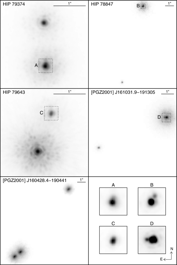
Figure 4. Triple systems identified in our survey. The intensity scale is logarithmic. Close-ups of the tight components of the first four triple systems are shown with a linear intensity scale on the bottom right panel.
Download figure:
Standard image High-resolution imageTable 5. Measurements and Properties of Multiple Systems
| Name | Separation | P.A. | ΔK | q |
|---|---|---|---|---|
| ('') | (deg) | (mag) | ||
| Binaries | ||||
| HIP 77840 | 2.061 ± 0.001 | 268.28 ± 0.02 | 1.89 ± 0.02 | 0.39 |
| HIP 79530a | 1.715 ± 0.001 | 219.23 ± 0.02 | 1.70 ± 0.01 | 0.39 |
| HIP 78530 | 4.529 ± 0.003 | 140.32 ± 0.02 | 7.26 ± 0.04 | 0.01 |
| HIP 78549a | 0.325 ± 0.001 | 189.06 ± 0.19 | 3.99 ± 0.03 | 0.07 |
| HIP 78956 | 1.060 ± 0.001 | 51.21 ± 0.03 | 1.47 ± 0.00 | 0.53 |
| HIP 79124 | 0.990 ± 0.001 | 98.11 ± 0.05 | 3.35 ± 0.04 | 0.14 |
| HIP 79156 | 0.880 ± 0.002 | 57.18 ± 0.10 | 3.33 ± 0.05 | 0.14 |
| HIP 79250 | 0.583 ± 0.002 | 178.07 ± 0.21 | 3.24 ± 0.05 | 0.18 |
| HIP 80059a | 0.245 ± 0.001 | 74.61 ± 0.11 | 2.36 ± 0.02 | 0.41 |
| HIP 78483 | 0.187 ± 0.001 | 161.47 ± 0.12 | 1.47 ± 0.01 | 0.78 |
| 1RXS J155500.0−234729 | 0.660 ± 0.001 | 241.28 ± 0.02 | 1.83 ± 0.01 | 0.57 |
| 1RXS J154106.9−265643 | 6.311 ± 0.003 | 82.45 ± 0.03 | 3.17 ± 0.01 | 0.15 |
| 1RXS J161329.9−231122 | 1.458 ± 0.002 | 91.45 ± 0.01 | 2.80 ± 0.02 | 0.11 |
| 1RXS J160251.5−240204 | 7.230 ± 0.002 | 353.59 ± 0.02 | 2.77 ± 0.04 | 0.10 |
| 1RXS J160210.1−224128 | 0.307 ± 0.001 | 325.84 ± 0.04 | 0.59 ± 0.00 | 0.64 |
| [PGZ2001] J160643.8−190805a | 0.247 ± 0.001 | 222.68 ± 0.12 | 1.70 ± 0.04 | 0.21 |
| 1RXS J160929.1−210524a | 2.213 ± 0.002 | 27.73 ± 0.06 | 7.26 ± 0.11 | 0.01 |
| 1RXS J155405.2−292032 | 1.434 ± 0.001 | 76.08 ± 0.01 | 1.33 ± 0.01 | 0.29 |
| [PZ99] J155716.6−252918 | 0.594 ± 0.001 | 323.22 ± 0.04 | 0.07 ± 0.00 | 0.94 |
| 1RXS J160355.8−203138 | 0.078 ± 0.001 | 345.77 ± 0.44 | 0.09 ± 0.03 | 0.92 |
| 1RXS J160621.5−192851 | 0.584 ± 0.001 | 139.84 ± 0.02 | 0.39 ± 0.01 | 0.71 |
| RX J155734.4−232112 | 0.051 ± 0.002 | 66.00 ± 2.00 | 1.00 ± 0.20 | 0.39 |
| 1RXS J160703.4−191138 | 0.611 ± 0.001 | 88.47 ± 0.03 | 1.57 ± 0.01 | 0.22 |
| [PGZ2001] J160823.8−193551 | 0.657 ± 0.001 | 64.96 ± 0.06 | 0.95 ± 0.01 | 0.41 |
| RX J155629.3−234821 | 0.146 ± 0.001 | 349.21 ± 0.09 | 0.10 ± 0.02 | 0.91 |
| 1RXS J160542.2−200413 | 0.613 ± 0.001 | 351.81 ± 0.02 | 0.45 ± 0.01 | 0.64 |
| 1RXS J160652.6−241627 | 1.688 ± 0.001 | 272.57 ± 0.02 | 0.53 ± 0.01 | 0.60 |
| [PGZ2001] J160801.5−192757a | 0.862 ± 0.001 | 313.90 ± 0.02 | 0.05 ± 0.01 | 0.95 |
| [PGZ2001] J161118.1−175728a | 0.098 ± 0.001 | 203.07 ± 0.39 | 0.05 ± 0.01 | 0.95 |
| Triples | ||||
| HIP 79374 Aa,Abb | 0.072 ± 0.001 | 346.35 ± 0.20 | 1.65 ± 0.03 | 0.46 |
| HIP 79374 Aa,Bb | 1.351 ± 0.001 | 1.80 ± 0.01 | 0.69 ± 0.10 | 0.72 |
| HIP 78847 Aa,Aba | 0.131 ± 0.001 | 329.17 ± 0.37 | 2.04 ± 0.04 | 0.39 |
| HIP 78847 Aa,B | 8.962 ± 0.001 | 164.74 ± 0.01 | 3.72 ± 0.08 | 0.10 |
| HIP 79643 A,Baa | 1.240 ± 0.002 | 340.33 ± 0.14 | 2.88 ± 0.03 | 0.36 |
| HIP 79643 Ba,Bba | 0.047 ± 0.003 | 336.77 ± 0.98 | 1.06 ± 0.04 | 0.38 |
| [PGZ2001] J161031.9−191305 Aa,Ab | 0.148 ± 0.004 | 84.00 ± 2.00 | 2.70 ± 0.15 | 0.09 |
| [PGZ2001] J161031.9−191305 Aa,B | 5.860 ± 0.001 | 113.81 ± 0.04 | 3.89 ± 0.06 | 0.04 |
| [PGZ2001] J160428.4−190441 Aa,Ab | 0.878 ± 0.001 | 128.49 ± 0.03 | 0.06 ± 0.02 | 0.95 |
| [PGZ2001] J160428.4−190441 Aa,B | 9.369 ± 0.001 | 322.49 ± 0.02 | 1.19 ± 0.04 | 0.34 |
Notes. aWe did not find previous mention of these companions in the literature. bMeasurements given are from the follow-up epoch.
Download table as: ASCIITypeset image
A pseudo-orbital period P' was calculated for each pair of stars assuming that the actual orbital semi-major axes are equal to 1.09 times the observed projected separations. We determined this average projection factor numerically following the approach described in the Appendix of Brandeker et al. (2006) and assuming a uniform eccentricity distribution, as observed for solar-type stars (Raghavan et al. 2010). Of the 34 binary pairs (including the 5 tight subsystems of the triples), 5 have a pseudo-orbital period of less than 50 yr (HIP 79374Aab, ∼10 yr; HIP 79643Bab, ∼17 yr; RX J155734.4−232112AB, ∼27 yr; 1RXS J160355.8−203138AB, ∼40 yr; HIP 78847Aab, ∼46 yr). For these, a partial orbit could be measured within the next 5–15 yr to derive dynamical constraints on their masses. All triple systems are in a stable configuration, with outer-to-inner period ratios largely exceeding the empirical stability limit of 5 (e.g., Tokovinin 2004).
Some of the main multiplicity properties of our sample are presented and briefly discussed in the following subsections. First, we present the multiplicity fraction (MF) and binary companion mass ratio distribution of our sample, which are frequently used as simple diagnostics of the formation process of multiple stars as they can be readily compared between various samples or against numerical results. We then investigate whether the presence of binary companions within our orbital separation range of sensitivity has a bearing on the presence of circumstellar disks. Finally, as the existence and origin of massive planets and low-mass brown dwarfs on wide orbits around stars is still largely unconstrained, and an active area of research, we determine their occurrence rate in our sample for intermediate and large orbital separations.
4.1. Multiplicity Fraction
The raw MF of our sample is 0.37 ± 0.05, while the mean number of companions per star, or companion star fraction (CSF), is 0.43 . The errors quoted are for 67% credibility and assume binomial statistics for the MF and Poisson statistics for the CSF. The raw MF and CSF should be viewed as strict lower limits as they are based on a sample that includes companions across a regime (separations from ∼005 to ∼9'' and contrasts of up to ∼7.5 mag) where our survey is incomplete due to varying levels of sensitivities for our different targets, as well as to a strong dependence of sensitivity with angular separation. Restricting instead to our complete sample, defined as including only the 80 targets for which the K-band magnitude limits achieved at all separations were at least as good as our 90% detection limits (from K < 9.3 at 01 to K < 15.8 at 5''; see Table 4), and considering only companions above those limits and with separations of 01–5'' (∼15–700 AU), the MF and CSF are 0.30 ± 0.05 and 0.30
 , respectively. The multiplicity values are significantly lower for the complete sample as several of the companions found fall outside of our completeness separation range.
As our sample was designed to have roughly equal numbers of stars in different logarithmic mass bins, its corresponding MF does not necessarily reflect the stellar population of Upper Sco. We can account for this by applying weights proportional to the initial mass function (IMF) to the systems observed. Doing so using a Kroupa IMF (Kroupa 2001), we obtain an MF and CSF of 0.37 ± 0.05 and 0.42 , respectively, for our raw sample; the effect here is thus negligible. Applying a similar correction to our complete sample, we obtain an MF and CSF of 0.27
 and 0.27
 , respectively, close to the uncorrected values. While useful to assess the effect of our mass-based target selection on the multiplicity statistics—which here turns out to be small—we note that making such a correction does introduce additional systematic errors, which stem from uncertainties about the universality and validity of the specific IMF used, as well as from uncertainties on the stellar mass estimates.
As for our survey for Cha I, we compare our results to those of the surveys of ρ Ophiuchus by Ratzka et al. (2005), of Taurus by Kohler & Leinert (1998), of the Orion Nebula cluster by Köhler et al. (2006), and of the IC 348 cluster by Duchêne et al. (1999). The latter two regions are dense star-forming regions, while the former, as well as Cha I and US, are more dispersed. We take the same approach as before and adapt our results to match the sensitivity regimes of the other surveys before making a comparison. For convenience, the statistics from these surveys are reproduced in Table 6, along with our new results. For the reasons given above, we do not attempt to correct our sample for the stellar IMF in making the comparisons. We first compare our new results for US with our previous results for the Cha I region. Considering the detection and separation limits corresponding to the complete Cha I sample of Lafrenière et al. (2008a), 01 < θ < 6'' and ΔK < 1.2 at 01 to <3.1 at 6'', the present survey yields an MF of 0.24 , compared with a value of 0.27
 for Cha I. The MF is thus the same in both regions in this regime of contrast and separation. Taken at face value, the CSF for this restricted sample is marginally lower in US (0.24
 ) than in Cha I (0.32
 ), but the difference is not statistically significant. As we find the same results within the statistical uncertainties for these two samples, we also merged them together to improve the statistics. Now considering a more restricted sample (013 < θ < 64, ΔK < 2.5, and K < 10.4), allowing comparison with a larger set of surveys, we obtain an MF of 0.23 ± 0.05 for US, which agrees within the uncertainties with the value of 0.28 ± 0.03 found for the other dispersed regions considered (Cha I+ρ Oph+Taurus). The comparison with the two denser regions, ONC and IC 348 (both requiring an even more restricted sample), does reveal a difference: the MFs in both US and Cha I are higher by factors of 2–3. The statistics from the merged US+Cha I sample indicate that the probabilities that their MF was drawn from the same underlying binomial distribution as for the ONC and IC 348 are only 2% and 6%, respectively.11 The higher occurrence of binaries by factors of two to three in more dispersed regions is thus statistically significant.
Table 6. Multiplicity Fractions of Various Samples
| Study | Region | N | B | T | MF | CSF |
|---|---|---|---|---|---|---|
| Raw sample | ||||||
| This work | US | 91 | 29 | 5 | 0.37 ± 0.05 | 0.43 |
| This work, IMF-weighted | US | 91 | 29.6a | 4.4a | 0.37 ± 0.05 | 0.42 |
| Complete sampleb | ||||||
| This work | US | 80 | 24 | 0 | 0.30 ± 0.05 | 0.30 |
| This work, IMF-weighted | US | 80 | 18.7a | 0 | 0.27 |
0.27 |
| Restricted sample (01 < θ < 6'' and ΔK < 90% limit of Lafrenière et al. 2008a) | ||||||
| This work | US | 88 | 21 | 0 | 0.24 |
0.24 |
| Lafrenière et al. (2008a) | Cha I | 110 | 25 | 5 |  |
 |
| Combined US+Cha I | ⋅⋅⋅ | 198 | 46 | 5 | 0.26 ± 0.03 | 0.28 ± 0.04 |
| Restricted sample (013 < θ < 64, ΔK < 2.5, and K < 10.4) | ||||||
| This work | US | 79 | 18 | 0 | 0.23 |
0.23 |
| Combined Cha I+ρ Oph+Taurusc | ⋅⋅⋅ | 278 | 72 | 5 | 0.28 ± 0.03 | 0.29 ± 0.03 |
| Restricted sample (0.1 < M/M☉ < 2.0, 60 < θ/AU < 500, and ΔK < 3.5) | ||||||
| This work | US | 57 | 10 | 0 | 0.18 |
⋅⋅⋅ |
| Lafrenière et al. (2008a) | Cha I | 96 | 13 | 0 |  |
⋅⋅⋅ |
| Combined US+Cha I | ⋅⋅⋅ | 153 | 23 | 0 | 0.15 ± 0.03 | ⋅⋅⋅ |
| Köhler et al. (2006) | ONC | 105 | 5.4 | 0 |  |
⋅⋅⋅ |
| Restricted sample (32 < θ/AU < 640 and q > 0.1) | ||||||
| This work | US | 83 | 21 | 0 | 0.25 |
⋅⋅⋅ |
| Lafrenière et al. (2008a) | Cha I | 76 | 18 | 0 |  |
⋅⋅⋅ |
| Combined US+Cha I | ⋅⋅⋅ | 159 | 39 | 0 |  |
⋅⋅⋅ |
| Duchêne et al. (1999) | IC 348 | 66 | 8.5 | 0 |  |
⋅⋅⋅ |
Notes.
aThe effective number is given, after applying the weights as explained in the text.
bConsidering only targets for which the K-band magnitude limits achieved at all separations were at least as good as our 90% detection limits (see Table 4), and considering only companions above those limits and with separations in 01–5''.
cSee Table 6 of Lafrenière et al. (2008a).
Download table as: ASCIITypeset image
Finally, we compare our MF to the value measured for the field. Assuming that the lognormal companion separation distribution observed by Raghavan et al. (2010) for field solar-type stars applies to stars of all masses, our orbital separation range of sensitivity (roughly 15–1000 AU for the combined US+Cha I sample) would contain 44% of all companions. This might be a slight overestimate, however, as the companion separation distribution of M-type stars, which dominate the IMF, has been found to differ from that of solar-type stars (Janson et al. 2012), being shifted toward smaller separations, although their specific distribution is unclear at the moment. Still, using this value in combination with the field IMF-weighted MF of about 0.33 reported by Lada (2006) leads to a field MF of 0.15 within our orbital separation range of sensitivity. The MF in the field is thus a factor of ∼2 below the value for the restricted US+Cha I sample (0.26), as well as a factor of ∼2 below the value for other dispersed star-forming regions per the above remarks.
Besides the overall MF of the sample, we have also divided our sample into four equal logarithmic mass bins and calculated the MF in each bin to investigate how these quantities vary with the primary star mass; the results are shown in Figure 5. Given the uncertainties in each bin, the distribution of MF in US appears to be consistent with being flat over the 0.2–7.5 M☉ range. Indeed, a straight line fit of the distribution returns a slope of 0.04 ± 0.13. In Figure 5, we also show the MF as a function of mass obtained for our Cha I survey. In the common regime of primary masses, the distributions in both regions agree well within the uncertainties. In the context of the generally accepted trend that multiplicity (integrated over all separations) rises and even becomes dominant at high masses (e.g., Raghavan et al. 2010; Janson et al. 2012; Kouwenhoven et al. 2007b; Delfosse et al. 2004; Siegler et al. 2005; Joergens 2008), the relative flatness of the MF distribution with mass observed in our US sample may be due to our limited orbital separation range, and does not necessarily indicate that the trend observed in the field does not hold for US. Indeed, differences in the companion orbital separation distributions with mass would mean that different fractions of the total population of binaries would be detected in our survey for different masses. For example, Duchêne & Kraus (2013) mention that the companion separation distribution for stars of mass 1.5–5 M☉ shows two main peaks, one falling well below our minimum separation limit and the other extending beyond our outer limit. On the other hand, the companion separation distributions of 0.2–1.5 M☉ stars roughly peak within our range of sensitivity. Thus, our completeness to binaries is likely lower for higher mass stars compared to lower mass ones. To illustrate that considering a restricted separation range can indeed affect the observed trend of MF with mass, we consider the results of Raghavan et al. (2010) for (field) G-type stars and of Janson et al. (2012) for (field) M-type stars. For M-type stars, Janson et al. find an MF of 0.27 ± 0.03 for the 3–227 AU separation range. For G-type stars, Raghavan et al. find an MF of 0.46 ± 0.02 over all separations, which, based on their companion separation distribution, translates into an MF of ∼0.21 for the 3–227 AU range. Thus, over this restricted separation range the MFs for G- and M-type stars are comparable, even though they are not when looking at the MF integrated over all separations. The relatively constant MF observed in our sample for a restricted separation range may thus be consistent with the trend observed in the field.

Figure 5. Multiplicity fraction of our US sample (solid histogram) as a function of primary star mass. The numbers shown in parentheses on the figure indicate the number of stars in each mass bin for our sample. For comparison, our results for Chamaeleon I (Lafrenière et al. 2008a) are also shown (dashed histogram).
Download figure:
Standard image High-resolution imageSurprisingly, we found only one multiple system among the eight primaries more massive than 7.5 M☉ that we observed (yielding an MF of 2.2%–35%). Various factors could explain this apparent discrepancy. First, as already mentioned above, a large fraction of binaries in this mass range could fall below our inner separation limit, as high-mass stars display a particularly high frequency of short-period binaries (Duchêne & Kraus 2013). Also, this mass limit (7.5 M☉) coincides with the star brightness at which we switched from using the full detector array to using only a 512 × 512 pixel subarray, and thus the companion search field of view is smaller (<750 AU) for these stars. As the more massive stars harbor companions out to larger orbital separations (≳ 104 AU; Duchêne & Kraus 2013), this could further reduce our completeness to companions for the most massive stars. In addition, as shown in Table 2, because of the different instrumental setup, the sensitivity limits reached for the most massive stars are generally about 2–4 mag worse than for typical targets (see also Table 4), which means that our completeness to low-mass companions is also reduced. In fact, from the mass ratio limits shown in Table 4 we can see that for the most massive stars we did not probe the full stellar companion regime for separations below 1''. Thus, we believe that our results for the highest mass stars should be interpreted with care. For these reasons we have not included this mass bin in Figure 5.
4.2. Mass Ratio of Binaries
Figure 6 shows the mass ratio distribution for all binary systems in our survey with q > 0.1 (regime in which our completeness is good). The distribution shows a higher incidence of lower mass ratio systems (0.1 < q < 0.4) compared to higher mass ratio ones. The rise is significant, as a Kolmogorov–Smirnov (K-S) test gives a probability of only 8% that the true underlying distribution is flat. For solar-type stars in the field, the observed mass ratio distribution is roughly uniform for q > 0.2 (Raghavan et al. 2010). At first glance, this seems to differ from what we observe here; however, this flat distribution is based on a sample that includes binary companions with separations below our inner separation limit, and these small separation companions were found to preferentially have higher mass ratios. Thus, their absence from our sample could explain the apparent difference. To study further the effect of orbital separation, Figure 6 also shows the mass ratio distributions when our sample is subdivided into binaries with projected orbital separations above or below 07 (∼100 AU). The trend noted above for the overall sample is even more pronounced for systems with wider separations, and a K-S test gives a probability of only 5% that the underlying distribution is uniform. On the other hand, the distribution looks flat for systems with small separations (∼15–100 AU). In this case, the K-S test gives a probability of 74% for a uniform distribution. There is thus a significant difference between the mass ratios of companions at separations of ∼15–100 AU versus those at larger separations, the latter preferentially having lower mass ratios. The exact same trend was also observed in our Cha I study, and in the studies of ρ Oph by Ratzka et al. (2005), of Sco-Cen by Köhler et al. (2000), and of Taurus by Kohler & Leinert (1998). This is also the case for field solar-type binaries (Duchêne & Kraus 2013), where it is observed that the mass ratio distribution of binaries with separations above ∼50 AU peaks at q ∼ 0.3. This is thus a rather common feature of binary systems.
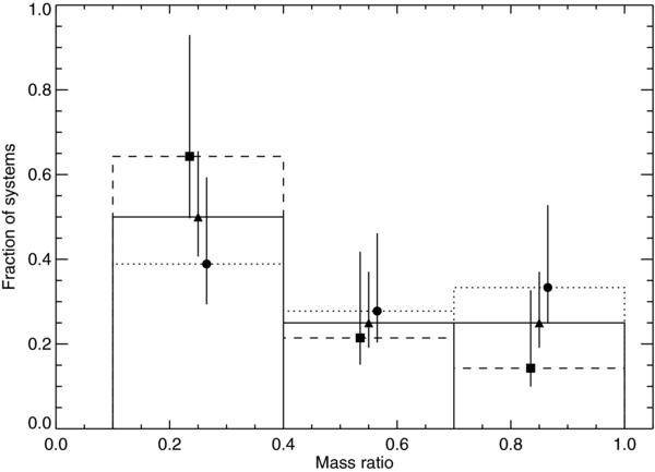
Figure 6. Mass ratio distributions for all binary systems with a mass ratio above 0.1 (solid histogram, triangles), as well as for the subsets of those systems with projected orbital separations above (dashed histogram, squares) and below (dotted histogram, circles) 07 (∼100 AU).
Download figure:
Standard image High-resolution imageFigure 7 shows the mass ratio of all binary systems as a function of primary mass. The figure shows an apparent lack of lower mass ratio companions around primaries of lower masses, as no companion with a mass ratio below 0.5 has been detected for primaries with masses below 0.4 M☉, despite good sensitivity to detect them beyond 025. A similar lack of low mass ratio companions at low primary masses was also observed in our Cha I study. These results seem to differ from what is observed for 0.1–0.5 M☉ stars in the field, where the observations are consistent with a more uniform companion mass ratio distribution for q > 0.1 (Janson et al. 2012), or only a modest decline at low mass ratios (Duchêne & Kraus 2013). Figure 7 also shows the mass ratios of the systems found in our Cha I study, where it seemed that more massive primaries had gradually lower mass ratio companions. In fact, the results in Cha I suggested a lower envelope on the mass ratio distribution that was roughly consistent with a constant companion mass (roughly coinciding with the stellar/substellar limit), possibly indicating that companion formation may become less efficient below a companion mass near the substellar limit. Given our detections of substellar companions, this is not readily apparent from our sample, although the relative number of substellar versus stellar companions found in our survey points in the same direction. In a regime where our observations are mostly complete to brown dwarf (0.012–0.072 M☉) companions, i.e., at >05 for 0.2 < M/M☉ ⩽ 0.5 and at >1'' for 0.5 < M/M☉ ⩽ 3.0, we have detected 13–14 stellar companions and two to three brown dwarf companions (depending on whether the tight companion to [PGZ2001] J161031.9−191305 is counted as stellar or substellar). The observed ratio of brown dwarf to stellar companions is thus  (67% credibility). Considering our sample of primary stars and assuming that the companion masses were drawn randomly from a Kroupa IMF (Kroupa 2001), then in the above regime of mass and separation our survey should have found 0.786 times as many brown dwarf companions as stellar ones, which is much higher than the observed ratio (the two values are inconsistent at 90% credibility). Thus, our data indicate that, as compared to formation in isolation, companion formation is less efficient in the brown dwarf mass regime than in the stellar mass regime.

Figure 7. Mass ratios of binary systems found in this study (diamonds) as a function of the primary masses. Filled symbols are for systems with a separation larger than 07 (∼100 AU), while open symbols are for smaller separations. The dotted lines show our 90% mass ratio detection limits for various angular separations (from bottom section of Table 4). The gray crosses show the systems found in the Cha I study of Lafrenière et al. (2008a). The dashed line marks the mass ratios for a companion at the substellar mass limit of 0.072 M☉, and the dot-dashed line marks the brown dwarf mass limit of 0.012 M☉.
Download figure:
Standard image High-resolution imageFigure 7 also suggests that there are fewer similar-mass binaries (q > 2/3) for higher mass primaries, compared to lower mass primaries: only 1 out of 13 binaries with primary masses of 1–3 M☉ has a mass ratio above 2/3, while it is the case for 7 out of 21 for binaries with primary masses of 0.2–1 M☉. The same trend was found in our study of Cha I (Lafrenière et al. 2008a), as well as for the A and B stars of Sco-Cen (Kouwenhoven et al. 2005).
4.3. Presence of Circumstellar Disks
As mentioned previously, all of our targets have been observed with Spitzer at 8, 16, 24, and 70 μm by Carpenter et al. (2006, 2009) to search for excess emission arising from circumstellar material. Carpenter et al. (2009) report excess emission due to a circumstellar disk for 18 of our 91 targets: 10 of them are classified as having a debris disk, and the other 8 as having a primordial disk. Among those 18 targets with disks, we find that 5 are multiple systems: HIP 78956 (debris), HIP 79156 (debris), HIP 79643 (debris), 1RXS J160621.5−192851 (primordial), and [PGZ2001] J160643.8−190805 (primordial). The fraction of multiple stars among stars with reported disks is thus 5/18 or 0.27 , which is to be compared with the fraction of multiple stars among stars without disk detection, 29/73 or 0.40 ± 0.06. The incidence of multiplicity may thus be marginally lower among disk-bearing stars, although the result is not statistically significant. Considering only our restricted sample, these fractions would be 4/14 (0.29
 ) and 20/66 (0.30
 ), respectively, and thus would be indistinguishable. Alternatively, we can look at the incidence of disks among multiple and single stars. For the raw samples, the numbers are, respectively, 5/34 (0.15
 ) and 13/57 (0.23
 ), while for the restricted sample they are, respectively, 4/24 (0.17
 ) and 10/56 (0.18
 ). Here again there is no difference. We note that the above comparisons are rather rough in that they do not take into account the various masses of the primaries, which are known to have an effect on the incidence, properties, and evolution of the disks; the statistics in our sample are insufficient to do a more in-depth analysis. We also note that the binary companions found in the systems with disks have projected separations of 40–260 AU, which is typically beyond the dust traced by the Spitzer observations.
4.4. Occurrence of Substellar Companions
The present study found two new low-mass substellar (≲40 MJup) companions—1RXS J160929.1−210524b and HIP 78530B (Lafrenière et al. 2008b, 2010, 2011; see also Ireland et al. 2011; Bailey et al. 2013)—and confirmed a previously known one, [PGZ2001] J161031.9−191305B (found by Kraus et al. 2008; see also Lachapelle et al. 2014). The latter is the outer member of a triple system in which the inner companion may itself be substellar as its mass is estimated to be about 0.07 M☉.
Following the Bayesian approach described in Lafrenière et al. (2007), we estimated the fraction of stars that harbor low-mass substellar companions at intermediate to large orbital separations. For each target, we first computed the completeness of our observations for companions of given masses and semi-major axes. For these Monte Carlo calculations, the companion eccentricities, mean anomalies, and orbital separation projection factors were drawn from a uniform distribution. For stars with a measured parallax, the distance was randomly sampled from a uniform distribution according to the measured value and associated uncertainty, while for the other stars the distance was sampled uniformly between 120 and 170 pc. The age of the stars was fixed at 5 Myr, and the DUSTY evolution models (Chabrier et al. 2000) were used to convert between masses and magnitudes in the K band. The mean completeness of our survey for various masses and semi-major axes is shown on Figure 8. As the figure shows, our observations generally offer good completeness for companions ≳25 MJup above ∼50 AU, while for companions of 4–5 MJup our completeness is good only for separations larger than ∼200 AU. Our completeness figure is of course affected by the assumed age and model uncertainties, but the effect is relatively small. For example, if the age were 10 Myr instead of 5 Myr, and if we assumed that the models were overluminous by one magnitude for a given mass, then the 50% completeness curve would shift upward by about 3 MJup and rightward by about 40 AU.

Figure 8. Mean completeness of our survey for substellar companions.
Download figure:
Standard image High-resolution image
Next, to constrain the fraction of stars with low-mass substellar companions, we considered the 5–40 MJup mass range, which safely encompasses the masses of the three detected companions mentioned above and safely avoids companions ambiguously near the stellar/substellar boundary. We assumed log-uniform mass and semi-major axis distributions, i.e., dN/dm∝m−1 and dN/da∝a−1. We have also made the calculations for two different semi-major axis ranges, 50–250 AU and 250–1000 AU, which are roughly equivalent in logarithmic space. The results are shown in Table 7. Our data indicate that less than 2.1% of US stars have a companion at 50–250 AU separation while 3.6 have one at 250–1000 AU. These statistics are insufficient to conclude firmly whether there is a difference between the companion populations at smaller and larger separation.
Table 7. Percentage of Stars Harboring 5–40 MJup Companions, at 67% Credibility
| Semi-major Axis | Sample | |||
|---|---|---|---|---|
| Range (AU) | Up Scoa | Up Sco+b | Cha Ic | GDPSd |
| Raw | ||||
| 50–250 | <2.1 | <1.8 | <1.2 | <1.7 |
| 250–1000 | 3.6 |
4.0 |
<1.3 | <5.7 |
| IMF-weighted | ||||
| 50–250 | <1.7 | <1.4 | <1.1 | <2.0 |
| 250–1000 | 1.8 |
3.2 |
<1.3 | <7.7 |
Notes. aThis work. bThis work + Kraus et al. (2008) + Ireland et al. (2011). cFrom Lafrenière et al. (2008a). dFrom Lafrenière et al. (2007).
Download table as: ASCIITypeset image
To improve the statistics, we merged the survey of US stars performed by Kraus et al. (2008) and Ireland et al. (2011) with ours. This adds 27 new stars to our sample and one substellar companion in a relevant mass and separation range (GSC 06214−00210B, ∼15 MJup, ∼320 AU; Ireland et al. 2011). For the augmented sample, the results indicate that less than 1.8% of stars have a low-mass substellar companion at 50–250 AU, while the fraction is 4.0 % for 250–1000 AU. Here the difference is statistically significant: from the posterior distributions we find that, with 84% credibility, the occurrence rate of 5–40 MJup companions is higher at large separations than at intermediate ones. This is in line with the trend mentioned earlier that larger separation companions can have lower mass ratios.
For comparison, we repeated the same exercise with two other samples for which we readily had access to the information needed: the AO multiplicity survey of the Chamaeleon I region from Lafrenière et al. (2008a) and the Gemini Deep Planet Survey (GDPS) from Lafrenière et al. (2007). The latter survey targeted nearby young and field stars of spectral types G, K, and M. Although our survey of Cha I was not as deep as the one here, it reached a similar completeness because that region is younger (2 Myr), making substellar objects of corresponding masses significantly brighter. Conversely, GDPS targeted nearby older stars of spectral types G, K, and M, but as it was deeper and reached better contrasts, it achieved similar completeness at 50–250 AU separations. However, it missed sensitivity to companions at 250–1000 AU as the closer target distances often made those separations fall out of the camera field of view. The comparison reveals that, with 88% credibility, the occurrence rate of substellar companions at 250–1000 AU is higher in US (4.0%) than in Cha I (<1.3%). However, the statistics are insufficient to draw any conclusion with respect to the older GDPS sample.
Finally, as done previously for the MF (Section 4.1), we have repeated the above calculations by factoring in the IMF to estimate values that may be more representative of the stellar population as a whole. In practice, this was done by raising each individual probability in the computation of the likelihood function to a power proportional to the probability of drawing the corresponding stellar mass from the IMF. These "powers," or weights, were normalized to have a mean of 1. Again, we used a Kroupa IMF. The results are shown in Table 7. The corrections are all small except for the US sample from this study and the 250–1000 AU separation range. In the latter case, as one of the three detected companions orbits a massive star, with a much lower weight, factoring in the IMF significantly reduced the calculated rate. In any case, all of the above conclusions still hold with the correction.
5. CONCLUDING REMARKS
The main findings of our survey are that for binary separations of a few tens to hundreds of AU, the MF in US is comparable to the MF in other dispersed star-forming regions, but is a factor of two to three higher than the MF in denser star-forming regions or in the field. Subdividing our sample based on stellar masses, we find that the MF is roughly constant with mass over the 0.2–7.5 M☉ range (and ∼15–1000 AU separations), although a modest rise in MF with mass cannot be formally ruled out given our statistics. We also find that wider binaries (>100 AU) and higher mass stars tend to preferentially have companions with lower companion-to-primary mass ratios. Eighteen stars in our sample harbor a circumstellar disk, but we have found no statistical difference regarding their multiplicity properties as compared to those without disks. Finally, we find an occurrence rate of low-mass substellar companions (5–40 MJup) of ∼4.0% for orbital separations of 250–1000 AU, compared to <1.8% at smaller separations. With an incidence rate of 4.0% in US, the low-mass substellar companions on orbits of hundreds of AU cannot be viewed as being exceptional, and thus their origin needs to be readily understood within the general framework of star and planet formation, a feat that will require more work from both the theoretical and the observational fronts.
The picture of the population of US multiples depicted here is far from complete, being limited both by the sample size and by the orbital separation range probed. A larger sample is needed to perform statistically significant comparisons of the properties of binary companions in different subsamples (primary masses, mass ratios, or orbital separations), as these can better reveal some aspect of their formation mechanism. Along the same line, extending the orbital separation range probed, apart from possibly revealing higher order multiples and uncovering the total companion population, would allow investigating the similarities or differences between the tightest and widest binary systems. Such a complete study would provide an excellent framework upon which to compare the results of theoretical modeling of the star formation processes, as well as the properties of the better studied field sample of multiple stars.
We thank our anonymous referee for a careful review of our manuscript and for excellent suggestions that helped improve this work. D.L. is supported in part through grants from the Natural Sciences and Engineering Research Council, Canada (NSERC), and the Fonds de Recherche du Québec—Nature et Technologies. Additional support for this work came from NSERC grants to R.J. and M.H.v.K. A.B. was supported by the Swedish National Space Board (contract 113/10:3).
Footnotes
- 5
Carpenter et al. (2006) mention that in selecting their targets, they removed from their initial compilation the stars for which a nearby star could compromise the Two Micron All Sky Survey (2MASS) photometry. Potentially, such a selection could preferentially weed out binaries and affect our multiplicity statistics. However, after verification (J. Carpenter 2013, private communication), only about 2% of their initial compilation was removed for this reason, and thus the effect on our statistics should be negligible.
- 6
As stated on the instrument Web site at http://www.gemini.edu/sciops/instruments/niri/imaging/pixel-scales-and-fov.
- 7
The distortion correction used is centro-symmetric and is given by r = r' + 1.32 × 10⁻⁵r'2, where r and r' are, respectively, the distortion-corrected and distorted radial pixel distances from the array center.
- 8
Imaging deeper than 2MASS has indeed verified that such an extrapolation is reasonable. For example, in a deep wide-area study of the Pleiades cluster, Lodieu et al. (2012) show that the logarithmic cumulative distribution of the number of sources as a function of magnitude is linear up to a K-band magnitude of ∼18.
- 9
We used the models with Y = 0.28, Z = 0.02, and XD = 2 × 10⁻⁵. We used the 1998 update of the models for masses in the range 0.017–0.9 M☉.
- 10
If the true age of US were 10 Myr instead of 5 Myr (see the discussion in the introduction), then the mass estimates would differ by up to 10%–20% from the values used here, while the mass ratios would typically differ by less than 10%.
- 11
Calculated using the test detailed in Appendix B2 of Brandeker et al. (2006).