


ABSTRACT
This paper provides a theory of using Liouville's theorem to map the anisotropy of TeV cosmic rays seen at Earth using the particle distribution function in the local interstellar medium (LISM). The ultimate source of cosmic ray anisotropy is the energy, pitch angle, and spatial dependence of the cosmic ray distribution function in the LISM. Because young nearby cosmic ray sources can make a special contribution to the cosmic ray anisotropy, the anisotropy depends on the source age, distance and magnetic connection, and particle diffusion of these cosmic rays, all of which make the anisotropy sensitive to the particle energy. When mapped through the magnetic and electric field of a magnetohydrodynamic model heliosphere, the large-scale dipolar and bidirectional interstellar anisotropy patterns become distorted if they are seen from Earth, resulting in many small structures in the observations. Best fits to cosmic ray anisotropy measurements have allowed us to estimate the particle density gradient and pitch angle anisotropies in the LISM. It is found that the heliotail, hydrogen deflection plane, and the plane perpendicular to the LISM magnetic field play a special role in distorting cosmic ray anisotropy. These features can lead to an accurate determination of the LISM magnetic field direction and polarity. The effects of solar cycle variation, the Sun's coronal magnetic field, and turbulence in the LISM and heliospheric magnetic fields are minor but clearly visible at a level roughly equal to a fraction of the overall anisotropy amplitude. The heliospheric influence becomes stronger at lower energies. Below 1 TeV, the anisotropy is dominated by small-scale patterns produced by disturbances in the heliosphere.
Export citation and abstract BibTeX RIS
1. INTRODUCTION
Recently, a great wealth of information about the directional variation (which is commonly referred to as anisotropy) in the flux of cosmic rays arriving at Earth in the TeV to PeV energy range has been obtained by quite a number of air shower experiments. Among those that have achieved excellent data quality with large event statistics are Tibet (Amenomori et al. 2006, 2010) Milagro (Abdo et al. 2008, 2009), Super-Kamiokande (Guilian et al. 2007), IceCube/EAS-Top (Abbasi et al. 2010, 2011, 2012), and ARGO-YGB (Di Sciascio et al. 2012). The observational results are quite surprising and, to some extent, confusing. Although there is a general large-scale anisotropy pattern with an amplitude of the order of 10−3, the data do not seem to fit any standard diffusion model of cosmic ray propagation through the interstellar medium with a typical magnetic field of a few μG and a large isotropic diffusion coefficient of ∼1028 cm2 s−1. The Compton–Getting effect due to the motion of the heliosphere relative to the local interstellar medium (LISM) is almost completely invisible. The phase of the large-scale anisotropy pattern shifts between 20 TeV and 400 TeV (Abbasi et al. 2012), which has clearly ruled out the theory that the Compton–Getting effect is a major source of the anisotropy. A more surprising feature is that there is clear evidence for small-scale structures of tens of degrees in angular size in the anisotropy data. Small regions of enhanced cosmic ray flux are called hot spots in some reports (e.g., Abdo et al. 2008). The amplitude of the small-scale anisotropy is roughly a fraction of the large-scale anisotropy, but the details of the small-scale anisotropy pattern are quite energy dependent and, to some extent, time dependent as well (e.g., Amenomori et al. 2006).
The source of these anisotropies is unknown. According to the standard diffusion theory of charged particles gyrating in a large-scale magnetic field, we would get a dipole anisotropy pattern regardless of whether or not there are multiple contributions from the Compton–Getting effect, diffusion, or the density gradient. With a more elaborated pitch angle diffusion theory, one would only get hot spots in the direction parallel or antiparallel to the magnetic field. Even if the large-scale magnetic field in the LISM is not uniform as suggested by Drury & Aharonian (2008), the focusing effect of the magnetic mirror would only produce a bidirectional anisotropy along the magnetic field. To overcome these difficulties, new theories beyond the standard diffusion theory have been proposed. Giacinti & Sigl (2012) argued that small-scale anisotropy can arise from scattering on the local magnetic field turbulence structures combined with the presence of a large-scale anisotropy. The apparent association of cosmic ray intensity enhancement with the heliotail has led to the suggestion that particle acceleration through magnetic reconnection in the heliotail might be responsible (Lazarian & Desiati 2010). On a similar note, Drury (2013) proposed that the electric field in the heliosphere might accelerate or decelerate cosmic rays to produce the small-scale anisotropy. Desiati & Lazarian (2013) argued that small structures of cosmic ray anisotropy might be produced from large-scale dipole interstellar anisotropy via perturbation from heliopsheric fields and interstellar magnetic turbulence within the particle mean free path. More recently, Schwadron et al. (2014) calculated some influence from the outer heliosheath magnetic field with constraints from IBEX observations of the energetic neutral atom (ENA) emission ribbon, but their work only covers limited aspects of all possible contributions. Even more fascinating, Kotera et al. (2013) speculated that the anisotropy might be due to neutral quark matter lumps of strangelets, which could be produced through interactions in molecular clouds.
While some of the above suggested theories are worth further exploration or detailed calculation, this paper concentrates on an investigation of the effect due to the presence of the heliosphere. The gyroradius of a particle with a momentum p and charge q in the magnetic field B is ρg = p/(qB). For 1 TeV protons in a typical 3 μG interstellar magnetic field, the gyroradius is only 74 AU. Our heliosphere is much bigger than that in all directions, and the heliotail might extend to several thousand AU. Drastically different heliospheric magnetic fields can significantly alter the trajectories of cosmic rays of up to PeV energy. Therefore, we expect some heliospheric distortion to the anisotropy pattern that would be seen in the LISM without heliospheric influence. We apply Liouville's theorem to map the cosmic ray distribution function from the local interstellar space to Earth at 1 AU from the Sun. The trajectories of cosmic rays are calculated from the electric and magnetic fields obtained by a magnetohydrodynamic (MHD) model simulation of the heliosphere.
2. THEORY
2.1. Principle of Flux Mapping
Anisotropy measures the directional variation of differential cosmic ray flux J in terms of the number of particles per unit area, solid angle, energy interval, and time interval. It is directly related to the particle distribution function f at the observer's location ro through:

where po is the particle momentum in the observer's own reference frame and po is its magnitude. Since we only care about the directional variation at a fixed particle energy or energy interval, the anisotropy of cosmic ray flux is just the directional variation of the particle distribution function in the observer's reference frame.
According to Liouville's theorem, the multi-particle distribution function of an ensemble is constant along the trajectory of a Hamiltonian canonical dynamical system. For space plasma, such as cosmic rays, we only consider the one-body distribution function, which is commonly referred to as the distribution function. Its evolution obeys the Boltzmann–Vlasov equation. The solution to it is still Liouville's theorem, but this time the distribution function is constant along the trajectory of a single particle. If the total electric and magnetic fields are given so that the particle trajectory can be calculated deterministically, we can the map cosmic ray distribution function at Earth to the far enough interstellar space where the cosmic ray distribution function is undisturbed by the presence of the heliosphere, i.e.,

where r and p are the location and momentum vectors anywhere along the trajectory of a particle starting at ro and po. Note that the particle distribution function is conserved upon transformation of the reference frame, so p and po do not have to be in the same reference frame as long as the momenta in different reference frames are related through a proper Lorentz transformation and the motion obeys Hamilton's equations.
In space plasma, there are always fast (in both time and spatial scales) varying components in the electric and magnetic fields commonly known as waves or turbulence, which are hard to determine at any given instant. When turbulence is present, the cosmic ray trajectories will exhibit a stochastic nature. If the perturbative force is small enough, an applicable quasilinear theory will always lead to particle diffusion in the phase space, in which the particle distribution function is governed by a Fokker–Planck diffusion equation. The solution to the diffusion equation can be expressed as the expectation value of the source particle distribution function sampled by stochastic trajectories, which is a superposition of a deterministic process governed by the Lorentz force in the average fields and a diffusion process driven by fluctuating fields (see, e.g., Zhang 1999). For 1 TeV cosmic ray protons, the scattering time by random electric and magnetic fields in the interstellar space, which is possibly on the order of 10 yr to have a mean free path of 3 pc, is very long compared to its gyro period of 2.7 days in a 3 μG magnetic field. Within the time on the order of a few days for the particle to traverse through the heliosphere, the particle trajectories do not deviate very much through scattering by magnetic field fluctuation. Therefore, we can almost map the distribution function deterministically by sampling just one particle trajectory.
Equation (2) forms the basis for calculating cosmic ray anisotropy observed at Earth. It also tells us that the anisotropy has to come from the anisotropy that already exists in the LISM. In other words, if the distribution function in the LISM were a constant, there would be no anisotropy at all. Therefore, we must analyze the possible sources of large-scale anisotropy in the LISM.
2.2. Sources of Anisotropy
The gyroradius of TeV cosmic rays is quite small compared to the scale size of the local interstellar magnetic field, which is tens or maybe hundreds of parsecs. These cosmic rays belong to a magnetized plasma, for which the theory of anisotropy is quite different from that of an unmagnetized particle population. In the limit of low scattering, if the magnetic field is not curved or inhomogeneous enough on the scale of a particle gyroradius, we expect that there will be a gyrotropic symmetry in the particle distribution function in the plasma reference frame where the electric field is zero. In the diffusion approximation that requires small anisotropy, the particle distribution function in the local interstellar magnetic field can be expressed as (Schlickeiser 2002):

where p is the particle momentum in the reference frame of the local interstellar magnetic field, p is its magnitude, μ is the cosine of particle pitch angle relative to the magnetic field direction, and Rg is the guiding center of the particle located at r. F(Rg, p) is an isotropic main component of cosmic ray distribution function. δf ≪ F is the pitch angle dependent part of the distribution function that comes from the diffusive perturbation. The variation in Equation (3) as a function of all the variables there constitutes the source of anisotropy.
First, the cosmic ray distribution function is energy or momentum dependent, which can be approximately written by a power law, F∝p−s with s ≈ 4.75. When the interstellar magnetic field is moving relative to an observer at a velocity of Vism (Vism ≪ c), the distribution function in the observer's reference frame is
We have used a Lorentz transform of momentum p = po − γm0Vism in the non-relativistic regime (Vism ≪ c). The particle has a rest mass of m0 and a Lorentz factor of γ. A Taylor expansion to the first order yields the familiar term of Compton–Getting dipole anisotropy  , where v is the particle speed v = po/(γm0) and
  is the direction of the incoming particle to the observer.
It can be seen that Compton–Getting anisotropy arises from the variation of the particle distribution function F(p) due to the angular dependence of particle momentum in the interstellar magnetic field reference frame p when the momentum is transformed from the observer's reference frame. We do not have to use the Taylor expansion to figure out the Compton–Getting anisotropy. Instead, we can directly calculate the function F(p) as the Lorentz transformation of momentum is performed for all different directions of  . This anisotropy determination method is more accurate because Vism does not have to be much less than v for non-relativistic particles, which is required in the first order Taylor expansion. In the presence of the heliosphere, the transfer of particle momentum observed at Earth to the momentum in the interstellar magnetic field must undergo an additional propagation through the electric and magnetic fields of the heliosphere. The motional electric field of the heliospheric plasma can change particle momentum as pointed out by Drury (2013) and particle acceleration inside magnetic reconnection sites can do the same (Lazarian & Desiati 2010). After the particle momentum is mapped to the interstellar space in the interstellar magnetic field reference frame, the change of momentum not only contains the effect of reference frame transformation but also the effect of particle acceleration. All these effects can be automatically included in the calculation of F(p) in Equation (4).
The second source of cosmic ray anisotropy comes from the spatial dependence of F(Rg). If there is a spatial gradient of cosmic ray density, the flux of particles coming from different directions will be different because of the displacement of their guiding centers. Mathematically,
where we have used the gyroradius vector  in the interstellar magnetic field Bism and a Taylor expansion to the first order of ρg. The dipole anisotropy
  is commonly called b cross gradient anisotropy, or it is sometimes called drift anisotropy, although the guiding center does not drift in a uniform magnetic field. Like Compton–Getting anisotropy, the calculation of b cross gradient anisotropy can be done by evaluating the distribution function at the guiding center
  . This calculation method is more accurate than the Taylor expansion approximation and can also handle the perturbation of particle trajectory by the heliospheric magnetic field.
The third source of anisotropy is the angular dependence in δf, which could be a function of gyrophase as well as pitch angle. Analysis of strongly magnetized plasma by Schlickeiser (2002) showed that the amplitude of pitch angle dependence is much larger than gyrophase dependence in a uniform averaged magnetic field. This point will be further elaborated later when we discuss the condition of the LISM. Under the diffusion approximation (Schlickeiser 2002), we can write
. This calculation method is more accurate than the Taylor expansion approximation and can also handle the perturbation of particle trajectory by the heliospheric magnetic field.
The third source of anisotropy is the angular dependence in δf, which could be a function of gyrophase as well as pitch angle. Analysis of strongly magnetized plasma by Schlickeiser (2002) showed that the amplitude of pitch angle dependence is much larger than gyrophase dependence in a uniform averaged magnetic field. This point will be further elaborated later when we discuss the condition of the LISM. Under the diffusion approximation (Schlickeiser 2002), we can write
where z is the coordinate of position along the magnetic field direction and Dμμ is the pitch angle diffusion coefficient. When the dominant pitch angle anisotropy is the first order term of μ due to a uniform angular (per degree) scattering rate with Dμμ = D0(1 − μ2) (D0 is a constant), the pitch angle anisotropy can be written in terms of parallel mean free path λ|| as

which is consistent with the dipole of diffusion anisotropy in the parallel direction. In general, the pitch angle anisotropy in the diffusion approximation of magnetized plasma does not have to be a dipole if the angular (per degree) scattering rate Dμμ/(1 − μ2) is not uniform. If the particles have not been sufficiently scattered after they are released from a point source, the pitch angle anisotropy can be beam-like or cone-like depending on the age since release. Multiple sources on both ends of the magnetic field line or particle reflection by magnetic mirrors can give rise to a bidirectional anisotropy. In other words, the pitch angle distribution function δf can have quite a number of possibilities even under the diffusion approximation. These possibilities will be investigated as input parameters in a harmonic expansion.
2.3. Cosmic Ray Anisotropy in the LISM
We know the cosmic ray spectrum and the solar system velocity relative to the LISM well enough to accurately figure out the amount of Compton–Getting anisotropy. At the measured speed of 26 km s−1, the amplitude of Compton–Getting anisotropy should be around 4 × 10⁻⁴, which is much lower than the observed anisotropy in the TeV cosmic ray flux. Furthermore, the direction of cosmic ray anisotropy is energy dependent and does not agree with the flow direction of the interstellar medium. All these factors indicate that anisotropies due to the cosmic ray density gradient, either through particle diffusion or the b cross gradient, are bigger contributors to the cosmic ray anisotropy. Unfortunately, we do not know anything about the spatial distribution of cosmic ray density in the LISM which is necessary in order to calculate diffusion or the b cross gradient anisotropy. We then have to rely on models to predict the possible levels for these anisotropies. It is found that the details of cosmic ray spatial distribution strongly depend on the past source of cosmic rays and the mode of cosmic ray propagation through the interstellar magnetic field. Cosmic ray propagation models assuming global continuous source injection and a uniform and isotropic diffusion in a completely randomized Galactic magnetic field often overpredicts the amount of cosmic ray anisotropy even if only for the dipole pattern (Strong et al. 2007). A good alternative is that one or a few nearby past supernova remnants make a significant contribution to the total flux of cosmic rays we see in the solar system. Model calculation (Ptuskin et al. 2006) with multiple random impulsive point sources shows that, in this scenario, cosmic ray enhancements from nearby supernova sources are sensitive to the level of diffusion coefficient and the age and distance of the source. This might be able to explain why the cosmic ray anisotropy behaves differently in different energy bands.
In models that assume anisotropic diffusion, even though each nearby point source produces a dipole anisotropy in the direction of the source, the total anisotropy is still a dipole no matter how many significant sources there are. In addition, since the mean free path used in these diffusion models is much larger than the particle gyroradius, the b cross gradient becomes negligible.
However, several recent observations seem to indicate that the magnetic field in the LISM up to tens of parsecs is not random enough to warrant isotropic diffusion. The first piece of evidence is from IBEX observations of a ribbon in the image of ENAs emitted from the interstellar medium immediately outside of the heliopause. The effective volume is perhaps a few tens to hundreds of AU. It is found that the ribbon is organized along the line of sight that is perpendicular to the local interstellar magnetic field line (McComas et al. 2009; Heerikhuisen et al. 2010). If the interstellar magnetic field were random, we would not have seen a thin ribbon organized by the magnetic field. Model calculation of particle transport in the local interstellar magnetic field suggests that the turbulence in the local interstellar magnetic field must be quite low (Gamayunov et al. 2010). The second piece of evidence is from measurements of the polarization of starlight. Frisch et al. (2010) compiled and analyzed the polarization data from many stars within 40 pc. They found that the large-scale magnetic field is well ordered and shows little curvature. The direction of the average field is consistent with the orientation of the IBEX ribbon and the fluctuation of the field direction is less than 23°, which probably includes uncertainty of measurements. They concluded that the interstellar magnetic field is relatively uniform over spatial scales of 8–200 pc.
If the interstellar magnetic field is well structured, we expect cosmic ray diffusion to be highly anisotropic. In the heliospheric magnetic field, although the turbulence energy is comparable to the average magnetic field energy, namely (δB/B)2 ∼ 1, the ratio of particle perpendicular diffusion to parallel diffusion κ⊥/κ|| is of the order of just a few percent. The turbulence in the local interstellar magnetic field is much weaker, as implied from the level of fluctuation in the magnetic field direction derived by Frisch et al. (2010). Thus, we argue that the ratio κ⊥/κ|| could be lower, perhaps lower than 10−3, for the majority of cosmic rays below PeV. In a magnetized plasma where scattering is weak, the parallel and perpendicular diffusion are related by (Axford 1965; Jokipii 1966; Isenberg & Jokipii 1979),
where κA = vρg/3 is usually called the antisymmetric element of the diffusion tensor. Compared to the value of κA, the diffusion coefficient typically used in the modeling of interstellar propagation such as in, e.g., Strong et al. (2007) is much larger. The diffusion is likely to be the result of parallel diffusion or κ||/κA ≫ 1, so the κ⊥/κ|| must be small. Efforts investigating cosmic ray interstellar propagation with anisotropic diffusion have been undertaken recently to explain high-energy gamma ray emissions (Nava & Gabici 2013; Giacinti et al. 2013) and to study the possible variation of the cosmic ray spectrum in the Galaxy (Effenberger et al. 2013). Here we employ anisotropy diffusion to argue that b cross gradient anisotropy could be a leading source of cosmic ray anisotropy.
Let us assume a nearby past supernova remnant makes a significant contribution to the cosmic rays we measure in the solar system in a particular energy band. The propagation from this local source is through anisotropic diffusion in an ordered magnetic field. For simplicity, we use a Cartesian coordinate system, although the real magnetic field line could be curved on a very large scale. The equation that governs that particle distribution function from the point source can be written as
where the point source is injected at time t1 and location r1. The solution to Equation (9) is
The gradient of cosmic rays from this local source is
Assume that the rest of the supernova remnant sources in the entire Galaxy form a continuous and uniform distribution Fc. Roughly, Fc can be estimated with  , where
  is the average supernova occurrence rate, Tres is the cosmic ray residence time, and
  is the volume of the Galaxy filled with these cosmic rays. Figure 1 shows an example spatial distribution of the total cosmic rays F = Fc + F1 normalized by Fc. The contour lines are the ratio of F1/(Fc + F1). It can be seen that the local enhancement of cosmic ray density contributed from the nearby point source only appears within a very elongated oval island. On most of the area of this island, the cosmic ray density gradient, which is inversely proportional to the distance between any two adjacent isointensity contours, is much larger in the perpendicular direction than in the parallel direction.
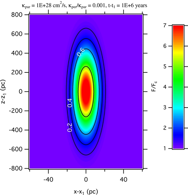
Figure 1. Cosmic ray intensity in the vicinity of a past supernova remnant. It is shown in units of continuous and uniform cosmic ray background. The contours indicate the ratio of local enhancement from the point source to the total intensity.
Download figure:
Standard image High-resolution imageThe dipole anisotropy vector from cosmic ray diffusion is
where  is the symmetric diffusion tensor containing κ|| and κ⊥. The diffusion anisotropy due to a single point source always points away from the point source. As anisotropy can only become significant on the very elongated island of local enhancement due to the factor of F1/(Fc + F1) in Equation (12), either the amplitude of diffusion anisotropy in the parallel direction is much larger than in the perpendicular direction (Figure 2) in most areas of the oval island, or the total diffusion anisotropy will be most likely to appear in the parallel direction—the farther away, the larger until the factor of flux ratio F1/(Fc + F1) becomes too small. This parallel diffusion anisotropy can be expressed as pitch angle anisotropy using δf from Equation (6).
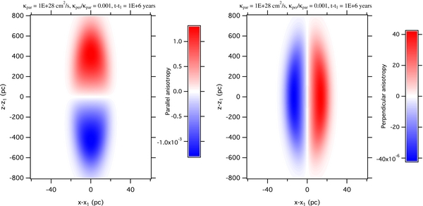
Figure 2. Amplitude of parallel (left) and perpendicular (right) diffusion anisotropy in the vicinity of a point source.
Download figure:
Standard image High-resolution imageThe dipole anisotropy vector from the b cross gradient in the perpendicular direction is
Compared with the diffusion anisotropy in Equation (12), the b cross gradient anisotropy is increased by a factor of κA/κ⊥ ratio in the perpendicular direction. This component could be comparable to or even larger than the pitch angle anisotropy in the parallel diffusion. Since the magnetic field strength and direction in the LISM is more or less known, the cosmic ray density gradient in the perpendicular direction is the major unknown parameter for determining b cross gradient anisotropy.
Notice that both the diffusion anisotropy in Equation (12) and b cross gradient anisotropy in Equation (13) are multiplied by a factor of F1/(Fc + F1). Only when F1 is comparable to or larger than Fc does the anisotropy from the local point source contribution become important. It turns out that the ratio F1/(Fc + F1) is sensitive to the particle diffusion coefficient and the distance and age of the source. This behavior can be easily seen in Figure 3. The diffusion coefficient is most likely to be particle energy dependent. Cosmic rays measured in one energy band in the solar system could contain a significant contribution from one or a few sources, but in another energy band, the cosmic ray local enhancement may come from another set of sources. Therefore, we expect that cosmic ray anisotropy in the LISM is quite energy dependent. The shift of phase in large-scale anisotropy from 20 TeV to 400 TeV should seem natural if the anisotropy contains a significant component of diffusion or b cross gradient anisotropy.

Figure 3. Temporal variations of cosmic ray intensity from a point source for three different values of the diffusion coefficient. They illustrate how a local enhancement from the point source comes and goes relative to a continuous uniform background.
Download figure:
Standard image High-resolution imageThe above demonstration of enhanced cosmic ray density and anisotropy from a local nearby young source employs an oversimplified Cartesian geometry. In reality, the Galactic magnetic field on a scale larger than 10–100's pc could be curved or even tightly folded, particularly near supernova remnants. The interstellar magnetic turbulence could contain high power at long wavelengths (Han et al. 2004) because of relative motion of interstellar clouds or disturbances driven by supernova explosions. In other words, magnetic field lines can appear to be meandering over large scales. On the small scale of the LISM, cosmic rays of these energies are still strongly magnetized, but there is little turbulence power at the wavelengths comparable to the particle gyro motion. In addition to this, particle perpendicular diffusion due to scattering by the turbulence is weak. As a result, cosmic rays tend to follow the local magnetic field lines, exhibiting density enhancements in the flux tube as a filament if it is connected to a recent source nearby. The cosmic ray density gradient across magnetic flux tubes is large, but perpendicular diffusion anisotropy is small due to the particle's inability to jump across field lines. When coupled with the meandering geometry of the Galactic magnetic field, cosmic rays on large scales may not necessarily appear to be very anisotropically distributed as shown in Figure 1 because filaments of enhanced cosmic rays can fold together (Giacinti et al. 2013). TeV gamma-ray observations by the Hess experiment (Aharonian et al. 2006) showed that cosmic rays are not very anisotropycally distributed around supernova remnants, probably because field lines have been strongly stirred by the supernova explosions. Therefore, while cosmic ray perpendicular diffusion is weak on the scale of the LISM, on large scales, cosmic ray transport may not be that anisotropic. Similarly, as a consequence of these particle transport behaviors, the cosmic ray density gradient in the LISM may be large due to the presence of filaments, but on large scales, cosmic ray distribution can be more uniform. The calculation of TeV cosmic ray anisotropy seen by experiments on Earth involves only the local cosmic ray distribution and particle transport behavior. Evidence for these behaviors of particle transport in turbulent magnetic fields of different scales has been observed in the heliosphere where the solar energetic particles from small solar flares tend to form sharp density discontinuities but the solar energetic particles from large-size coronal mass ejections tend to spread easily over solar longitude and latitude (Mazur et al. 2000).
Cosmic ray anisotropy in the LISM ultimately is the source of the anisotropy we see at Earth even though the deflection of the particle trajectory by the heliospheric magnetic field and the acceleration by the heliospheric electric field can distort the anisotropy. The distribution function as a function of particle moment, pitch angle, and guiding center position in the LISM become a boundary condition, which is needed to use Liouville's theorem to map the interstellar anisotropy to the anisotropy we see at Earth. Let us write the interstellar cosmic ray distribution function in a perturbation form as
where F0 is a constant value of f at a reference guiding center R0 at the observer's location, and P1(μ) and P2(μ) are the first and second order Legendre polynomials of pitch angle cosine μ. The rest constant parameters that govern the local interstellar cosmic ray variation are the spectral slope s, the amplitude and polarity of the dipole moment A1|| and the amplitude of bidirectional anisotropy A2|| in the pitch angle dependence, and the perpendicular gradient vector of cosmic ray density ∇⊥ln F. We have neglected the parallel gradient because it is expected to be much smaller than the perpendicular one, as shown in Figure 1. The four parameters, A1||, A2||, and ∇⊥ln F (a 2D vector) could be slightly energy dependent, as cosmic ray interstellar propagation is sensitive to diffusion coefficients, local interstellar magnetic geometry, and the age and distance of the local source.
2.4. Heliospheric Propagation
The propagation of TeV cosmic rays through the heliosphere is almost deterministic because the particle scattering time by the interstellar turbulence is much longer than the propagation time. Their trajectory is governed by the Lorentz force
where we only need to know the average electric E and magnetic B fields everywhere the entire heliosphere and the surroundings.
We use a model of the outer heliosphere that is commonly accepted to be among the most sophisticated models (e.g., Pogorelov et al. 2013 and references therein). This model and a corresponding package of numerical codes supporting it (the Multi-Scale FLUid-Kinetic Simulation Suite, MS-FLUKSS) uses an ideal MHD treatment of ions and a kinetic (or multi-fluid) description of neutral interstellar particles penetrating into the heliosphere. It addresses the complexity of the charge-exchange processes and coupling of the interstellar and heliospheric magnetic fields at the heliospheric interface. It has been used to analyze the influence of the interstellar environment on the heliospheric interface and has allowed us to investigate a number of sophisticated solar-wind–interstellar-medium interactions. This model was compared with the first IBEX measurements (McComas et al. 2009) and reproduced the ENA ribbon (Heerikhuisen et al. 2010). The comparison has put a very tight constraint on the direction of the local interstellar magnetic field outside of the heliopause (Heerikhuisen & Pogorelov 2011; Pogorelov et al. 2010, Pogorelov et al. 2011; Heerikhuisen et al. 2014). However, only in situ measurements performed by Voyager 1 (Burlaga & Ness 2014) can determine the exact polarity (Borovikov & Pogorelov 2014), provided that Voyager 1 is confirmed to have crossed the heliopause in 2012 August.
Figure 4 shows an example of magnetic field strength in the meridional plane (Figure 4(B)) and equatorial plane (Figure 4(A)), where the x-axis points toward the helionose in the ecliptic equatorial plane and the z-axis is in the direction of the north ecliptic pole, or approximately, the solar rotation axis. The interstellar magnetic field at infinity is 3 μG with a polar angle to the z-axis equal to 60° and an azimuth angle of 342° to the x-axis (ecliptic latitude 30° and ecliptic longitude 241°; or declination 9° and right ascension 245°). The heliotail in which the magnetic field is much weaker than the interstellar magnetic field could extend to a few thousand AU. The heliotail will eventually collapse to a small section due to the presence of the pressure from the interstellar neutral atom. In addition, the interstellar magnetic field can gradually diffuse into the tail, reaching a nearly uniform magnetic field there. In this MHD simulation of the heliosphere, the outer boundary is set at 1000 AU. We assume that the magnetic field beyond the simulation box shown in Figure 4 is the undisturbed uniform interstellar magnetic field. When cosmic ray particles propagate in a magnetic field of nearly uniform interstellar field strength and direction, their energy, pitch angle, and perpendicular guiding center remain constant, so the result of flux mapping does not need to specify where the interstellar boundary is as long as the magnetic field has become close enough to the interstellar value and the particles will no longer gyrate back into the heliopsheric influence.
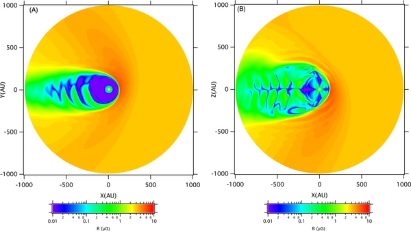
Figure 4. Strength of the magnetic field in the solar equatorial (A) and meridional (B) planes.
Download figure:
Standard image High-resolution imageSince this MHD heliosphere model run focuses on the large-scale interaction between the solar wind and interstellar medium, the simulation starts at 10 AU. The magnetic field close to the Sun is very strong, although it decays quickly within a few AU. The trajectories of TeV cosmic rays can be severely affected by the solar magnetic field. Thus, we use the Parker solar wind and heliospheric magnetic field model within 10 AU of the Sun. The title angle of the heliospheric current sheet, polarity of the solar magnetic field, and solar wind speed are calculated by matching the inner boundary of the MHD run. The azimuthal phase of the heliospheric current sheet tilt is also derived from the boundary condition.
Among the model outputs of the MHD heliosphere simulation are plasma velocity V and magnetic field B vectors. Since the plasma obeys the laws of an ideal MHD system, which is expected to be true everywhere except inside the tiny regions (approximately ion inertia length) where magnetic reconnection occurs, the electric field is to drive the plasma motion, i.e.,

Although the force on cosmic rays from the electric field is much weaker than the force by the magnetic field, the electric field can change the energy of cosmic rays. This can alter the behavior of Compton–Getting anisotropy.
The MHD model is run in the solar reference frame, so the plasma velocity and calculated electric field are also in the solar frame. For convenience, we also solve the Newton equation with Lorentz force (15) in the solar reference frame. The momentum of cosmic rays as measured at Earth first transformed into the solar frame, which should be season dependent. However, if we only investigate the yearly averaged anisotropy measurements, the seasonal effect due to Earth's motion around the Sun should be mostly averaged out. Thus, for the purpose of comparing with the yearly average of measurement, we run the model from a stationary Earth at 1 AU. The trajectories of cosmic rays are traced back in time until reaching the undisturbed interstellar magnetic field. The momentum is then transformed into the reference frame comoving with the LISM. The magnitude of momentum, pitch angle, and position of guiding center in the interstellar reference frame are used to calculate cosmic ray flux using Equation (14). Some sample trajectories will be shown later to aid in the understanding of some particular behaviors of cosmic ray propagation when our anisotropy calculation results are presented.
3. RESULTS
3.1. Compton–Getting Effect
The original Compton–Getting effect comes from the transformation of the reference frame when an observer is moving relative to an isotropic particle distribution in the plasma reference frame. Here in this paper, we expand Compton–Getting anisotropy to include the effect of energy gain or loss from the particle motion in the electric field of the solar wind and the heliosheath.
Figure 5 shows a map of a normalized particle distribution function (top) and its deviation from the original Compton–Getting computation (bottom) as a function of the right ascension α and declination δ in the celestial equatorial coordinate system. This calculation is done for one frame snapshot of a time-dependent MHD heliosphere run, in which the heliospheric current sheet tilts about 13 5 in a negative solar magnetic polarity cycle. It roughly corresponds to a solar minimum condition. The time is set when the Sun is in front of Earth toward the helionose and the phase of the heliopsheric current sheet tilt at the Sun points toward approximately 300° longitude in the xyz coordinates. The distribution is computed from the final particle momentum in the interstellar medium reference frame, pism, when the particle has completely escaped the outer heliospheric boundary by more than one particle gyroradius. The normalized distribution function is
where s = 4.75 is the slope of the cosmic ray distribution function and po = 6 TeV/c is the arrival particle momentum observed at Earth.
The Compton–Getting anisotropy of 6 TeV energy protons in Figure 5 is shown in the stationary Earth frame. This angular distribution (top panel) is dominated by a dipole derived from the motion of the heliosphere relative to the LISM. Subtracting the dipole distribution of the original Compton–Getting effect, we get an angular distribution of the deviation (Δ Compton–Getting anisotropy in the bottom panel), which is the result of energy gain or loss when the particles propagate through the electric field of the heliosphere. The maximum range of deviation is set to 2.5 × 10⁻⁴ with a slight saturation of color occurring in some of the areas. The effect of heliospheric influence is obvious with the highest deviation occurring on a warped ring slightly offset from the plane perpendicular to the unperturbed LISM (the dashed line). In some parts of the ring, large deviation splits into two bands, one of which has enhancement of cosmic ray intensity while in the other, cosmic rays are depressed. The magnitude of the deviation in the plane perpendicular to the unperturbed local interstellar magnetic field can be comparable to the amplitude of the original Compton–Getting anisotropy ∼4 × 10⁻⁴. In the direction near the helionose, Figure 5 shows an effect from the magnetic field of the solar corona and inner heliosphere. There are also a few regions of moderate levels of deviation in the Compton–Getting anisotropy. These are the result of particle drift across the surfaces of isoelectric potential in the heliosphere.

Figure 5. Cosmic ray anisotropy induced by a combination of the Compton–Getting effect and particle energy change during heliospheric propagation (top) and its deviation from the standard Compton–Getting anisotropy due to the motion of the heliosphere in the LISM (bottom). The solid sine curve is the ecliptic plane. The dashed curve is the plane perpendicular to the local interstellar magnetic Bism. The dash-dotted curve is the plane containing the vectors of local interstellar magnetic field and interstellar flow, or in short, the B − V plane.
Download figure:
Standard image High-resolution image3.2. Pitch Angle Anisotropy
The pitch angle dependence of the interstellar distribution function can be distorted by particle propagation through the heliospheric magnetic field. The distortion can be determined by tracing the particle pitch angle cosine relative to the reference frame of the interstellar magnetic field μism backward in time until reaching its steady level in the uniform interstellar field. The μism distribution is actually the particle pitch angle cosine before it enters into the heliospheric influence. A map of μism as a function of arrival declination and right ascension is shown in the top panel of Figure 6(A). The cosmic ray pitch angle anisotropy is just a simple function of the μism map, either in the first order or second order Legendre polynomial. In the case of the first order polynomial, the pitch angle anisotropy map is just proportional to the μism subject to a proportional constant A1|| known as the amplitude of unidirectional anisotropy. Bidirectional pitch angle anisotropy is proportional to the second order polynomial (3μism − 1)/2) subject to a constant amplitude A2||.
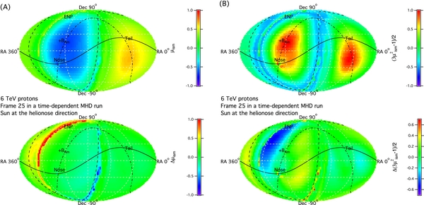
Figure 6. Maps of the first (A) and second (B) Legendre order polynomials of the incoming particle pitch angle cosine in the interstellar medium μism and the deviations from their values of the final pitch angle cosine at Earth.
Download figure:
Standard image High-resolution imageAs shown by Figure 6(A), the μism distribution is mostly a dipole in the direction opposite to the uniform interstellar magnetic field. Subtracting out the dipole, we obtain a map of deviation in the pitch angle cosine Δμism due to particle propagation through the non-uniform field in the outer heliosheath and the solar wind. Large deviations are seen on the warped ring offset from the plane perpendicular to the unperturbed local interstellar magnetic field. The level of the deviation in some areas is close to 1 or −1, indicating the particles have reversed the direction of its guiding center motion. The smaller deviation of μism from the dipole can be seen in a few other areas, such as the Sun's direction (at the helionose). The bidirectional anisotropy and its deviation from the original quadruple distribution are shown in Figure 6(B). This time, the deviation becomes more obvious due to the color scheme, particularly the double band structure of the offset from the plane perpendicular to the unperturbed local interstellar magnetic field shown in the top panel. Other areas also display deviation when the scale range is slightly reduced.
3.3. B Cross Gradient Anisotropy
This anisotropy comes from the displacement particle guiding center as a function of particle arrival direction. The result is an inner product of the spatial gradient of cosmic ray density ∇⊥ln f and the displacement of the guiding center d = Rg − R0. Usually, the cosmic ray density parallel to the magnetic field is much smaller than in the perpendicular direction due to larger parallel diffusion, so we do not compute the parallel component of the guiding center displacement. Since the gradient vector is a free parameter, it is better to show the displacement vector in the direction perpendicular to the local interstellar magnetic field. The perpendicular vector is divided into two orthogonal components. The first component is along a unit vector  , which points to the intersection between the ecliptic plane and the plane perpendicular to the unperturbed local interstellar magnetic field in the maps (declination −11° and right ascension 332°). The other component finishes the right-hand coordinates with the local interstellar magnetic field direction, i.e.,
  . The results of two guiding center displacement vector components and their deviation from their dipole distribution in the uniform interstellar magnetic field are shown in Figure 7.
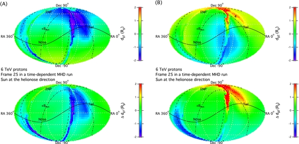
Figure 7. Maps of perpendicular guiding center displacement along  (A) and
  (B) and the difference from their respective displacements in a uniform interstellar magnetic field.
Download figure:
Standard image High-resolution imageThe dipole anisotropy produced by the guiding center displacement due to a unit density gradient  points toward the direction of their cross product (declination −75° and right ascension 192°), which can barely be seen by the yellowish green area in the top panel of Figure 7(A) to the color scale used. The deviation of the guiding center displacement due to the non-uniform heliospheric magnetic field is bigger than 1 gyroradius, as shown in the bottom panel of Figure 6(A). Most of the guiding center displacements are negative, indicating that the particles drift toward the negative
  direction. The effect of the plane perpendicular to the unperturbed local interstellar magnetic field is still there, and now the effect of the heliotail becomes visible too. The helotail is slight shifted and elongated along the B − V plane (the dash-dotted line), which contains the interstellar magnetic field vector and interstellar flow vector pointing from the helionose to the heliotail. Due to magnetic pressure exerted by the interstellar magentic field (ISMF) draped around the heliopause, the heliotail rotates and becomes aligned with the BV plane. The heliopause and the heliotail are also compressed by the ISMF, so that their "flaring" is noticeably greater in the BV plane than in the plane perpendicular to it while still containing the unperturbed LISM velocity vector.
The anisotropy produced by the other unit density gradient component  is shown in Figure 7(B). The dipole that would be produced in the uniform interstellar magnetic field points toward the direction of
  , as indicated by the slight enhancement of yellow color in that direction and by the more obvious enhancement of light blue color in the opposite direction. The deviation of the guiding center displacement from the original dipole is larger, particularly in the warped ring offset from the plane perpendicular to the unperturbed local interstellar magnetic field and the heliotail elongated along the B–V plane.
3.4. Sample Trajectories
Figure 8 shows some sample trajectories of Eo = 6 TeV particles arriving in several characteristic directions labeled "Nose," "Tail," "3," and "4" in Figure 7(B). Note that the time axis is backward. When the particle completely exits the heliospheric influence, its momentum (pism), pitch angle cosine (μism), and perpendicular guiding center location in the interstellar medium reference frame no longer change, so our simulation does not have to have a precise boundary as long as the particle has left the heliosphere by more than 1 gyroradius.
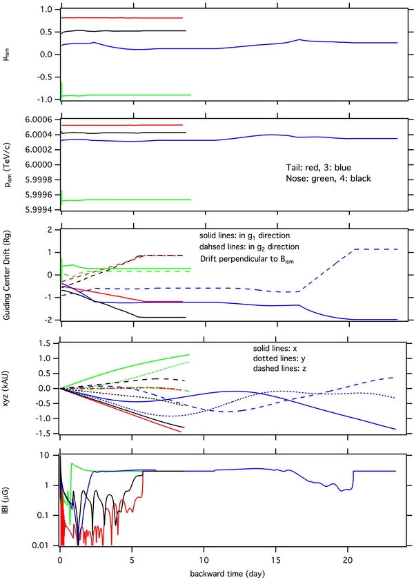
Figure 8. From top to bottom: backward time variation of the pitch angle cosine, momentum, and perpendicular guiding center components in the local interstellar magnetic field reference frame, Cartesian coordinates of particle position relative to the Sun, and the magnetic field strength experienced along four color-coded sample trajectories.
Download figure:
Standard image High-resolution imageIn the helionose direction (green curves), the trajectory starts with a moderate pitch angle cosine μism and the thickness of the heliosphere is small, so the particle takes a small amount of time to go through the heliospheric field. There is little drift in pism and μism and the guiding center location, resulting in small deviations from their original dipole anisotropies. At the beginning of the curves, there is a glitch in all these quantities because in this particular trajectory, the particle passes through the solar corona where the magnetic field is strong enough to alter the trajectory significantly in a very short distance.
The trajectory that arrives in the direction of the heliotail (red) also starts with a moderate pitch angle cosine, so the particle can go through the heliotail quickly. There are some small energy and pitch angle changes during the propagation, which result in a slight deviation from the original Compton–Getting anisotropy and pitch angle anisotropy. However, there is quite an amount of drift in the guiding center when the particle propagates through the heliotail where the magnetic field strength is much weaker than in the interstellar field.
In the directions close to the plane perpendicular to the interstellar magnetic field (3: blue curves), the particle starts with a small pitch angle cosine from 0. The particle spends more time in the vicinity of the heliotail. Every time it passes through the weaker heliotail magnetic field, its guiding center drifts rapidly. While there are some variations of particle energy and pitch angle, the drift in the guiding center dominates this part of the trajectory. Combining this with the long propagation time, the particle has a greater chance of drifting farther away in all the variables. This is the major reason why we see strong deviations near the plane perpendicular to the unperturbed local interstellar magnetic field. A slight offset from the exact plane perpendicular to the interstellar magnetic field is expected because the particle can be deflected by the high nonuniform heliospheric magnetic field.
For the particle arriving in the direction of (4: black curves), it passes through the heliotail with a large drift in its guiding center. The behavior is very similar to the particle arriving exactly in the heliotail direction (red curves). In this sense, the strong deviation in the B − V plane toward the northern tail direction comes from the same effect of the heliotail. The direction is not exactly along the tail because the particle is deflected by the heliospheric magnetic field.
3.5. Composite Anisotropy
As expressed by Equation (14), the total anisotropy observed by cosmic ray experiments is a linear combination of the above three types of anisotropy: Compton–Getting, pitch angle, and b cross gradient. Compton–Getting anisotropy is pretty much fixed due to the certainty of the cosmic ray energy spectrum. The pitch angle anisotropy has two parameters: the amplitudes of the unidirectional and bidirectional anisotropies A1|| and A2||. The b cross gradient anisotropy is subject to two free parameters: the two components of the cosmic ray density gradient vector in the plane perpendicular to the interstellar magnetic field ∇⊥ln F. Due to the complexity of the heliosphere-distortion pattern of these three types of anisotropy, different combinations of the four free parameters can look vastly different in the composite anisotropy map. The effects of the plane perpendicular to the unperturbed local interstellar magnetic field and the hellotail that show up in each individual component of the three types of anisotropy can cancel each other out or amplify each other. Some of the features may or may not show up in the composite anisotropy.
In order to understand the physical reality in the observations of cosmic ray anisotropy, it is necessary to determine how much each of the three types of anisotropy contributes to the whole. We choose to use a least χ2 method to fit observational data with Equation (14). Since the distributions of p, Rg − R0, and μ under heliospheric influence have already been calculated in the above, what is left unknown are the four linear parameters A1||, A2||,  , and
, and  . A minimization procedure similar to the common linear regression by setting the derivatives of χ2 to zero can allow us to determine the best fit parameters. We apply this procedure to cosmic ray anisotropy measurements at 6 TeV energy from the Tibet ASγ experiment. As a matter of fact, so far, we have not obtained the original data. Instead, we use synthetic data that are generated from the best fits to the original Tibet ASγ data with a superposition of two orthogonal dipoles and one bidirectional distribution (Amenomori et al. 2009; Mizoguchi et al. 2009).
The best fit composite anisotropy map is shown in Figure 9. The top is the total anisotropy, which fits the synthetic Tibet ASγ to a somewhat satisfactory degree according to examination by eye. It shows a large-scale pattern: enhancement in the heliotail direction and depression in the helionose direction. There are also some patterns in the intermediate scale that can be picked up more easily if we enhance the scale range. The middle panel of Figure 9 is a superposition of three dipole distributions (Compton–Getting, unidirectional pitch angle, and b cross gradient) plus a bidirectional pitch angle distribution along the interstellar magnetic field of our heliosphere model. The bottom panel is the difference map, showing the distortion made by the presence of the heliosphere. Features left in the difference map are the elongated heliotail along the B − V plane and the warped ring offset from the plane perpendicular to the unperturbed local interstellar magnetic field. The B − V plane has been thought to be the hydrogen deflection plane of either Lallement et al. (2005) or Gurnett et al. (2006). Numerical simulations (Pogorelov et al. 2008, Pogorelov et al. 2009) showed that the deflection of interstellar neutral hydrogen flow occurs in the B−V plane. The coincidence of cosmic ray enhancement has been pointed by the Tibet ASγ team (Amenomori et al. 2009; Amenomori et al. 2009). Now, through this simulation, we understand it is produced by the drift of the particle guiding center in the elongated heliotail. In our simulation, we also see the warped ring offset from the plane perpendicular to the unperturbed local interstellar magnetic field. In the Tibet ASγ observations, there seem to be hints of cosmic ray intensity enhancement in some areas along the ring. It is hoped that this simulation will provide some guidance to confirm that such a feature exists in the data, and vice versa, if these features are proven, we can further refine the determination of the interstellar magnetic field direction.

Figure 9. Top: map of composite anisotropy from Equation (14) with best fit parameters in Table 1, (middle) map of a superposition of dipoles and bidirectional anisotropies in the LISM without heliospheric influence, and (bottom) the difference between the top and middle maps.
Download figure:
Standard image High-resolution imageThe best parameters to fit the Tibet ASγ 6 TeV cosmic ray anisotropy and their uncertainties are listed in Table 1. Table 2 lists the directions of the original LISM anistropies associated with these four parameters. Their magnitudes and directions can lead us to understand what causes the observed cosmic ray anisotropy and how TeV cosmic rays are distributed in the LISM.
Table 1. Best-fit Parameters in Equation (14) to Tibet ASγ 6 TeV Cosmic Ray Anisotropy
| A1||(%) | A2||(%) |  |
 |
|---|---|---|---|
| 0.121 ± 0.002 | 0.051 ± 0.003 | −0.058 ± 0.001 | 0.041 ± 0.001 |
Download table as: ASCIITypeset image
The cause of cosmic ray enhancement in the heliotail is mainly due to the pitch angle anisotropy in the interstellar medium. This is not necessarily a heliospheric effect. The unidirectional pitch angle anisotropy, which is related to the parallel cosmic ray density gradient through Equation (6), points roughly to the heliotail direction with an amplitude of 0.121%, which is almost three times stronger than the Compton–Getting anisotropy due the motion of the heliosphere in the helionose direction. It almost entirely cancels out the Compton–Getting effect. The bidirectional pitch angle anisotropy further increases the cosmic ray intensity in the heliotail, and in the meantime, it produces a slight elevation of cosmic ray intensity along the interstellar magnetic field direction, which results in some truncation of the blue region from a dipole distribution in the top and middle panels of Figure 9. This feature has been seen by the Tibet ASγ experiment. Furthermore, the perpendicular density gradient vector has a negative value in the  component, which reverses the deep blue color in Figure 7(A) to red color, and its
  component is positive to maintain the color scheme of the cosmic ray intensity. Both density gradient components enhance the cosmic ray intensity in the heliotail. The cosmic ray intensity enhancement caused by the particle density gradient in the heliotail is a heliospheric effect.
In the middle panel of Figure 9 is a superposition of three unidirectional dipole anisotropies and a bidirectional pitch angle anisotropy that would exist without the influence of the heliosphere. These anisotropies are organized strictly according to the directions of the interstellar magnetic field and interstellar flow. In the best fit performed by the Tibet ASγ team (Amenomori et al. 2009; Mizoguchi et al. 2009), only two dipole anisotropies and one bidirectional anisotropy are taken into account, so their derived magnetic field direction (constrained along the bidirectional anisotropy) has to be moved significantly away from the interstellar magnetic field of our model. With the IBEX observation of a ribbon in ENA emissions, we know that the interstellar magnetic field direction cannot be that far off from our heliosphere model. This discrepancy is solved now due to the fact that the physics allow us to include three unidirectional dipole anisotropies and our best fit does not have to move the interstellar magnetic field direction.
When we subtract the dipole and bidirectional anisotropies from the total composite anisotropy, we get the difference map at the bottom panel of Figure 9. The major features are the enhancements in cosmic ray intensity along the B−V plane and the warped ring of the plane perpendicular to the unperturbed local interstellar magnetic field. These enhancements are mainly due to the perpendicular density gradient. Calculated from its two components listed in Table 1, the magnitude of the perpendicular density gradient is |∇⊥ln F| = 0.071%/Rg, which translates to 0.160%/kAU for the 6 TeV cosmic ray protons with a gyroradius Rg = 445 AU in a 3 μG interstellar magnetic field. The direction of the perpendicular density gradient points to declination 46° and right ascension 144°, which is roughly in the direction of cosmic ray enhancements. When the particle travels inside the tail lobe of a low magnetic field, its guiding center drifts along the density gradients, resulting in a high intensity. In other words, the cosmic rays seen in these directions come from a region of interstellar space where the cosmic ray density is higher than those arriving in other directions. In addition, there appear to be a few weaker features in the difference map. The effect of the plane perpendicular to the unperturbed local interstellar magnetic field still remains at high declinations in the southern hemisphere. It is hoped that these features can be confirmed by the ICECUBE experiment.
3.6. Polarity of the Interstellar Magnetic Field
While recent Voyager in situ magnetic field measurements after the heliopause crossing in 2012 August (Burlaga et al. 2013; Burlaga & Ness 2014) have made us more confident about the polarity of interstellar magnetic field, we showed in the above that all MHD models, including ours, cannot tell the difference in its effect on the plasma structure of the heliosphere. Cosmic ray anisotropy can be used to diagnose the polarity because the deflection of cosmic rays and the drift of the guiding center are sensitive to the polarity of the local interstellar magnetic field. Figure 10 shows our calculation of 6 TeV cosmic ray proton anisotropy with the same plasma parameters except the interstellar magnetic field is reversed. The heliospheric magnetic field remains the same. The dipole and bidirectional anisotropies remain the same as before, as shown by the middle panel. For this to occur, both the unidirectional pitch angle anisotropy and the direction of the particle density gradient have to switch to the opposite directions. Under the influence of the heliosphere, the total composite anisotropy (top) looks quite different now and it does not resemble what is seen by the Tibet ASγ experiment. In the difference map (bottom), the effect of the heliotail is still there; however, the cosmic ray intensity has a deficit instead of an enhancement. The deficit is cause by particle drift against the cosmic ray density gradient. The feature produced by the plane perpendicular to the unperturbed local interstellar magnetic field shifts to the other side and makes the anisotropy pattern more complex on the helionose side. These features are not consistent with the Tibet ASγ observation. Therefore, we are more confident in saying that the local interstellar magnetic field goes from the southern into the northern hemisphere.
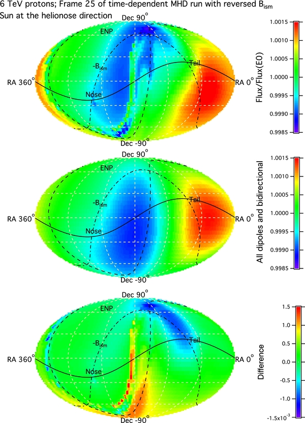
Figure 10. Composite anisotropy in the same format as in Figure 9 with a reversed interstellar magnetic field.
Download figure:
Standard image High-resolution image3.7. Solar Cycle Variation
Figure 11 shows our calculations for different phases of the solar cycle. Parameters of the interstellar dipole and bidirectional anisotropies remain the same as above. The MHD heliosphere models used are snapshots of the heliospheric configuration, which we label according to frame numbers in our MHD output. Major characteristics of the solar magnetic field conditions in the three frames are listed in Table 3. They correspond to two solar minima with opposite solar magnetic polarities and one solar maximum.

Figure 11. Composite anisotropy and its heliospheric distortion at two different phases of the solar cycle in Table 3.
Download figure:
Standard image High-resolution imageTable 2. Vector Direction
| Vector | Declination (δ) | Right Ascension (α) |
|---|---|---|
| Bism | 9° | 245° |
| Vism | −18° | 258° |
 |
−11° | 332° |
 |
75° | 12° |
Download table as: ASCIITypeset image
Table 3. Solar Magnetic Field Parameters
| MHD Model Frame Number | Solar Activity | HCS Tilt Angle | Polarity |
|---|---|---|---|
| 5 | Minimum | 10° | Positive |
| 15 | Maximum | 79° | Negative |
| 25 | Minimum | 135 |
Negative |
Download table as: ASCIITypeset image
The overall or large-scale pattern of 6 TeV cosmic ray anisotropy does not change much with the solar cycle. The features produced by the heliotail and the plane perpendicular to the unperturbed local interstellar magnetic field are still visible. The fact that the heliospheric magnetic field does not affect the anisotropy pattern very much is because that particle trajectory inside the heliopause is almost a straight line for particles of this energy so that the polarity of the heliospheric magnetic field does not matter much. However, more careful examination of the difference maps for the three MHD heliosphere frames can yield subtle differences in cosmic ray anisotropy at the level of ∼10−4. For example, there is a region of weak cosmic ray depression (light blue color) near the lower right side of the difference maps. The location and depression level moves significantly over the solar cycles. It is hoped that this feature can be confirmed by the ICECUBE experiment.
3.8. Solar Corona and Inner Heliospheric Magnetic Field
In the simulations in which we fix the Sun's location in the sky, we can clearly see the effect of magnetic field in the corona as well as in the inner heliosphere. The Sun's magnetic field can significantly bend TeV cosmic rays, causing their energy, pitch angle, and guiding center to drift as shown by the glitch in Figure 8 when the particle passes through the outer solar corona. In Figure 9, the Sun is located in the direction of the helionose. Distortion of cosmic ray anisotropy around it can be as much as 6 × 10⁻⁴. Should an investigation look into the anisotropy at this level, the effect of the Sun and its magnetic field around it must be considered. Figure 12 enhances the anisotropy difference map of Figure 9 by three times.
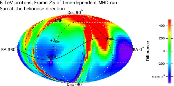
Figure 12. Difference map in Figure 8 with a smaller scale to highlight the influence of the Sun's coronal and inner heliospheric magnetic field.
Download figure:
Standard image High-resolution image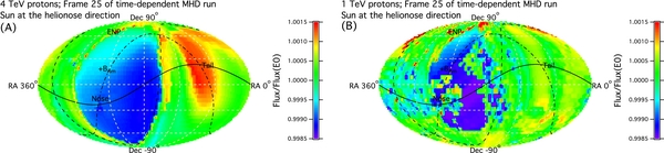
Figure 13. Maps of composite anisotropy of 4 TeV protons (A) and 1 TeV protons.
Download figure:
Standard image High-resolution imageAs the Sun moves over the sky along the ecliptic plane (the solid line), its direct influence on the cosmic ray anisotropy spreads. On a yearly average map, the effect may not be that dramatic. Since the distortion by the Sun's magnetic field spreads over many tens of degrees, its effect on the yearly average can still be around 10−4. An ideal simulation would have to sum over these distortions as the Sun moves in the sky. In addition, there is a possibility that the phase of the heliospheric current sheet may change the distortion pattern by the Sun's magnetic field. A spin average might be needed before the year average. All of these factors require further investigation. Our snapshots of the heliosphere do not have the time resolution to cover the Sun's spin, so we need a time-dependent heliosphere with a time cadence to resolve the Sun's spin.
3.9. Energy Dependence
The energy dependence of cosmic ray anisotropy is expected. Not only should the interstellar cosmic ray distribution evolve with energy, but also the distortion caused by the heliosphere should show up because of a strong dependence of the particle gyroradius on energy.
In Figure 13, we simulate the cosmic ray anisotropy at 4 TeV and 1 TeV. The amplitude of unidirectional and bidirectional pitch angle anisotropies and the perpendicular density gradient in units of percent/kAU are kept the same. The overall pattern for 4 TeV cosmic rays is roughly the same as 6 TeV in Figure 9. However, the anisotropy pattern of 1 TeV cosmic rays looks very different. Although there appears to be an overall deficit of cosmic rays toward the helionose side, the anisotropy is more dominated by the small-scale variations. There is hint that the effect of the heliotail is still there too. These features have been observed by the Milagro experiment. There are hot spots of cosmic ray enhancement at several places. The location of these spots, however, is very sensitive to our model parameters. In addition, the effect of the coronal and inner heliospheric magnetic field of the Sun, which is placed in the helionose direction in this simulation, becomes more prominent for the 1 TeV cosmic rays. All of these things tell us that the heliospheric influence is far more important at 1 TeV. This is expected as the gyroradius of 1 TeV protons is merely 74 AU in a 3 μG magnetic field.
Our calculations find that this heliosphere model of 1000 AU in radius is not adequate for cosmic rays of higher energies. For example, the gyroradius of 20 TeV protons is 1520 AU, which is larger than the size of the heliosphere simulation. Distortion by this model heliosphere is too small and smooth compared to observations by the Tibet ASγ and ICECUBE experiments. Improvement of the heliosphere model with a larger size is needed for studying higher-energy cosmic rays.
4. DISCUSSION
We have presented a method of using Liouville's theorem to map TeV cosmic ray anisotropies from the interstellar medium to the sky seen from Earth. We assume that the local interstellar cosmic ray distribution as a function of particle momentum, pitch angle, and spatial coordinates of the guiding center is a smooth function. We also assume that the trajectories of cosmic rays traversing through the heliosphere are deterministic under the Lorentz force in the average magnetic field and electric field. If these conditions are violated significantly, the Liouville mapping using merely one trajectory may become problematic and a new scheme of anisotropy mapping might be necessary. Let us look at now at how much violation there should be before this method becomes less useful.
4.1. Effect of Magnetic Turbulence
Turbulence in the heliospheric and interstellar magnetic field is ubiquitous. The magnetic field produced by MHD simulations does not include turbulence. Turbulence fluctuates rather quickly in time and space, which makes it impossible to include in the Lorentz force. Furthermore, cosmic ray particles arriving at different times experience different sets of magnetic perturbation along their trajectories of propagation. In this case, the trajectory becomes stochastic to those who only know the average fields. Now, the question is, can the stochasticity from the heliospheric and interstellar turbulence invalidate the method of Liouville mapping with a deterministic trajectory in the average fields?
To answer this question, we do some case studies in which the magnetic field of our heliosphere model is perturbed by an ad hoc fluctuation. If the result of cosmic ray anisotropy, particularly a specific feature of the anisotropy pattern, is not washed away completely by the added magnetic fluctuation, we can say the Liouville mapping with a deterministic trajectory is good enough. Otherwise, we need to do an ensemble average under the presence of the entire spectrum of magnetic turbulence, which is a different theory for calculating cosmic ray anisotropy.
Let us look at the cosmic ray anisotropy map when magnetic turbulence is added into the average field of the MHD heliosphere model. Since the properties of heliospheric magnetic turbulence are completely different from those of interstellar magnetic turbulence, we present our results for each separately.
Because it is constantly driven by the Sun, which emits supersonic and highly varying streams of solar wind, the turbulence in the heliospheric magnetic field is large even on small scales. To TeV cosmic rays, the particles are sensing the fluctuating magnetic field below the wavenumber corresponding to the correlation length. Given a typical Kolmogorov spectrum of magnetic turbulence, the fluctuating field sensed by TeV cosmic rays is almost at the level of the entire magnetic fluctuation spectrum. The  in the solar wind. We use a Gaussian random number with a standard deviation of 0.5B0 to generate a fluctuating magnetic field and add it to the perpendicular components of the average heliospheric field in each of the MHD simulation cells. The resulting anisotropy map of 6 TeV cosmic rays under an instant set of magnetic field fluctuation does not change much from the earlier results, so we do not show a similar map again. This is expected because even though we have a solar cycle variation with the heliospheric magnetic field flipping to the opposite polarity, we still do not see many changes in the TeV cosmic ray anisotropy. The physical reason for this is that the heliospheric magnetic field is too weak and too small in size to bend the TeV cosmic ray trajectory very much.
The properties of the local interstellar magnetic turbulence are less certain. We expect that it should be weaker than the heliospheric turbulence on the same scale size because there are fewer perturbation drivers in the interstellar medium to generate the turbulence and, more importantly, to overcome the most common effect of Landau damping. Small interstellar turbulence is implied from the IBEX observation of a ribbon in ENA emissions. In situ measurements of Voyager 1 outside of the heliopause also confirm small fluctuations in the interstellar magnetic field. A simulation run with an interstellar turbulence level of  is shown in Figure 14(A), in which there is little change in the TeV cosmic ray anisotropy pattern from our earlier results. However, TeV cosmic rays access magnetic turbulence on a much larger scale than the particles measured by IBEX and by the Voyager 1 spacecraft itself. If the Kolmogorov spectrum continues to low wave numbers, the fluctuation level seen by the TeV cosmic rays could be much larger. In Figure 14(B), we increase
  to 25%. There, the effect of fluctuation begins to be visible, but it again does not destroy the overall pattern of anisotropy produced by the interstellar cosmic ray distribution and the heliospheric structure. It should be noted that the effect of turbulence may become larger when we incorporate a larger heliosphere as the particles stay in the system longer during the propagation through the heliosphere. Should the interstellar turbulence become important, the trajectory of cosmic rays would exhibit a stochastic nature. Calculation of cosmic ray anisotropy requires an ensemble average.

Figure 14. Maps of composite anisotropy and their heliospheric distortions under a weak (A) and strong (B) large-scale interstellar turbulence.
Download figure:
Standard image High-resolution image
4.2. Fluctuation of Cosmic Ray Distribution in the LISM
When we map the anisotropy along the comic ray trajectories, we start with a smooth function of cosmic ray distribution in the LISM. If there is a fluctuation of the magnetic field in the interstellar medium, the cosmic ray distribution should exhibit a fluctuation too. In fact, it is this fluctuation that drives the cosmic ray diffusion through the Galaxy. The possible contribution of interstellar fluctuation to TeV cosmic ray anisotropy has been explored recently by Giacinti & Sigl (2012) and Desiati & Lazarian (2013) It is possible that we need it to explain small-scale anisotropy. However, the interstellar magnetic fluctuation alone can only produce a random pattern of anisotropy. Even so, it still relies on a large-scale inhomogeneity in the cosmic ray distribution to generate the small-scale fluctuation by interstellar turbulence as, according to the standard quasilinear theory (e.g., Schlickeiser 2002),
where xσ, (σ = 1, ...6) are the coordinates in the phase space (guiding center and momentum),  is the rate of change in particle motion driven by magnetic and electric perturbations, and the integration is carried out along the line of characteristics of particle helical motion in the average magnetic field. Thus, the fluctuating small-scale anisotropy is again the result of the average particle density gradient in all the variables such as spatial coordinates, pitch angle, and energy. The formula for the rate of change
  can be found in Schlickeiser (2002). Since its meaning is exactly the derivative of the phase space coordinates, i.e.,
the integration is performed over a total derivative and the result of the integration becomes

which is consistent with Liouville's theorem. This is expected because the governing equation is also the Boltzmann–Vlasov equation. Thus, the calculation of small-scale anisotropy due to the interstellar magnetic field turbulence is exactly the Liouville mapping if a magnetic fluctuation can be prescribed. An example has already been provided in the previous subsection. For the specific realization of interstellar magnetic turbulence  = 25% as shown in Figure 14(B), the small-scale anisotropy is visibly seen at the level of 10−4, approximately an order of magnitude lower than the large-scale anisotropy. Of course, the small-scale anisotropy level can be changed using different correlation lengths and randomness. If the large-scale interstellar magnetic turbulence varies more rapidly than the duration of the observation, it is necessary to make the ensemble average over the fluctuating field.
5. CONCLUSION
We have developed a method for the calculation of TeV cosmic ray anisotropy under the influence of the heliosphere. It is based on Liouville's theorem, which states that the particle distribution function is a constant of motion along the trajectory of particles under the total Lorentz force, so we can directly map the interstellar distribution function to the anisotropy sky seen from Earth deep inside the heliosphere. Mapping the anisotropy from the interstellar medium to Earth can also be done under the additional transformation of the reference frame between the observer frame and the interstellar plasma frame with a conservation of the particle distribution function.
We apply this method to TeV cosmic rays propagating through an MHD model heliosphere. We make the following conclusions from this initial study.
- 1.The ultimate source of anisotropy observed in cosmic ray is the inhomogeneity of the cosmic ray distribution function in the LISM. The cosmic ray distribution is a function of particle energy, pitch angle, and guiding center position. Any variation of cosmic ray distribution function with these variables contributes to the anisotropy observed at Earth as well as in the LISM.
- 2.Aside from the variation due to the average cosmic ray source distribution and its transport in the entire Galaxy, young and nearby sources of cosmic rays can make a special contribution to the anisotropy by local enhancement of cosmic ray density over the continuous global background. Such a local contribution from one or a few young point sources sensitively depends on the age, distance, magnetic connection, and particle diffusion coefficient. Thus, cosmic ray anisotropy sensitively depends on particle energy, at least in the energy band.
- 3.Compton–Getting anisotropy comes from the energy dependence of the cosmic ray distribution function. The motion of an observer relative to the interstellar plasma with which cosmic rays comove introduces an angular dependence of particle energy in the interstellar plasma reference frame. This is the original concept of Compton–Getting anisotropy. When cosmic rays propagate through the heliosphere, the heliospheric electric field can alter the particle energy. This is an additional source of anisotropy that may cause deviation from the original Compton–Getting dipole anisotropy.
- 4.A density gradient along the interstellar magnetic field gives rise to a pitch angle anisotropy. A unidirectional dipole pitch angle anisotropy is only a leading consequence of the parallel diffusion or pitch angle diffusion. Bidirectional pitch angle anisotropy is possible if the magnetic field flux tube is not uniform or there are multiple sources on the both ends of the flux tube.
- 5.Due to a small perpendicular diffusion of cosmic rays in an ordered magnetic field of the LISM, cosmic ray anisotropy in the direction perpendicular to the magnetic field comes mainly from b cross gradient anisotropy. The source of this anisotropy is the cosmic ray density gradient across the magnetic field.
- 6.Through the calculation of the particle trajectory that tracks the particle guiding center, pitch angle, and energy in the reference frame of the local interstellar magnetic field, we can trace where the cosmic ray anisotropy and its heliospheric distortion come from. The anisotropy and its distortion is most sensitive to the presence of the heliosphere in the direction approximately perpendicular to the local interstellar magnetic field or in the direction of the heliotail.
- 7.Fits to the measurements of anisotropy in 6 TeV cosmic rays demonstrate that the large-scale cosmic ray anisotropy in the LISM is composed of a unidirectional pitch angle anisotropy, a bidirectional pitch angle anisotropy in the direction parallel to the interstellar magnetic field, plus a contribution from the b cross cosmic ray density gradient perpendicular to the interstellar magnetic field. The amplitude of the pitch angle anisotropies and cosmic ray density gradient in the LISM can be determined. This information can give us some clues about the cosmic ray distribution in the LISM and possible young nearby cosmic ray source.
- 8.After the measurement of cosmic ray anisotropy has been subtracted from the dipole and bidirectional components of the local interstellar anisotropy, the remainder contains the effect of distortion by the heliosphere. In the Tibet ASγ observation, the reported cosmic ray enhancement along the hydrogen deflection plane (Amenomori et al. 2009) is consistent with our calculation of cosmic ray enhancement in the elongated heliotail along the B−V plane. We also find that additional features of cosmic ray enhancement along the partial ring are offset from the plane perpendicular to the local interstellar magnetic field. These features of cosmic ray enhancements can further constrain the direction and polarity of the local interstellar magnetic field.
- 9.The solar cycle variation of the heliospheric magnetic field and electric field makes minor but visible changes in the TeV cosmic ray anisotropy. The turbulence of the heliospheric magnetic field only plays a minor role.
- 10.The magnetic field in the solar corona and inner heliosphere make a minor but visible contribution to anisotropy. This may open up a possibility of using cosmic ray anisotropy measurements as a magnetic tomography of the Sun and its surroundings.
- 11.There is a clear energy dependence in cosmic ray anisotropy. From 4 TeV to 6 TeV, the overall pattern of anisotropy does not change much, but around 1 TeV, the anisotropy pattern changes dramatically. Although hints of a large-scale pattern of original interstellar anisotropy are still observable, the anisotropy of 1 TeV is more dominated by small-scale patterns produced by the heliospheric magnetic field. Hot spots of comic ray enhancement can appear at many places and their locations seem to be sensitive to the parameters of cosmic ray distribution in the LISM.
- 12.We agree with the claim by Giacinti & Sigl (2012) and Desiati & Lazarian (2013) that magnetic turbulence in the LISM can also produce small-scale fluctuation in cosmic ray anisotropy. Such a small anisotropy can only grow out of the large-scale anisotropy or inhomogeneities in the LISM. The size and the magnitude of the small-scale fluctuation could depend on the detailed properties of interstellar magnetic turbulence, such as the correlation length and turbulence energy. It is unclear whether an ensemble average over magnetic fluctuation can wash out or diminish this effect. Further study is needed.
This work was supported in part by NSF grant AGS-1156056; NASA grants NNX09AG29G, NNX09AB24G, and NNX10AE46G; and DOE grant DE-SC0008721. M.Z. would like to thank Julia Becker for an initial discussion that made him interested in the subject. We appreciate useful discussions with A. Lazarian and P. Desiati. We highly appreciate discussions at the team meeting "Heliosheath Processes and Structure of the Heliopause: Modeling Energetic Particles, Cosmic Rays, and Magnetic Fields" supported by the International Space Science Institute in Bern, Switzerland. We acknowledge NSF MRI grant 0923050, NSF PRAC award OCI-1144120, and related computer resources from the Blue Waters sustained-petascale computing project. Supercomputer time allocations were also provided on SGI Pleiades by NASA High-End Computing Program award SMD-14-4868 and Cray XT5 Kraken by NSF XSEDE project MCA07S033.