


ABSTRACT
We present a far-ultraviolet spectrum of the K4 Ib-II supergiant λ Vel obtained with the Hubble Space Telescope's Cosmic Origins Spectrograph (COS) as a part of the SNAPshot program "SNAPing coronal iron" (GO 11687). The observation covers a wavelength region (1326–1467 Å) not previously recorded for λ Vel at a spectral resolving power of R ∼ 20,000 and displays strong emission and absorption features, superposed on a bright chromospheric continuum. Fluorescent excitation is responsible for much of the observed emission, mainly powered by strong H i Lyα and the O i (UV 2) triplet emission near λ1304. The molecular CO and H2 fluorescences are weaker than in the early-K giant α Boo while the Fe ii and Cr ii lines, also pumped by H i Lyα, are stronger in λ Vel. This pattern of relative line strengths between the two stars is explained by the lower iron-group element abundance in α Boo, which weakens that star's Fe ii and Cr ii emission without reducing the molecular fluorescences. The λ Vel spectrum shows fluorescent Fe ii, Cr ii, and H2 emission similar to that observed in the M supergiant α Ori, but more numerous well-defined narrow emissions from CO. The additional CO emissions are visible in the spectrum of λ Vel since that star does not have the cool, opaque circumstellar shells that surround α Ori and produce broad circumstellar CO (A-X) band absorptions that hide those emissions in the cooler star. The presence of Si iv emission in λ Vel indicates a ∼8 × 10⁴ K plasma that is mixed into the cooler chromosphere. Evidence of the stellar wind is seen in the C ii λλ1334,1335 lines and in the blueshifted Fe ii and Ni ii wind absorption lines. Line modeling using Sobolev with Exact Integration for the C ii lines indicates a larger terminal velocity (∼45 versus ∼30 km s−1) and turbulence (∼27 versus <21 km s−1) with a more quickly accelerating wind (β = 0.35 versus 0.7) at the time of this COS observation in 2010 than derived from Goddard High Resolution Spectrograph data obtained in 1994. The Fe ii and Ni ii absorptions are blueshifted by 7.6 km s−1 relative to the chromospheric emission, suggesting formation in lower levels of the accelerating wind and their widths indicate a higher turbulence in the λ Vel wind compared to α Ori.
Export citation and abstract BibTeX RIS
1. INTRODUCTION
The Hubble Space Telescope (HST) SNAPshot program "SNAPing Coronal Iron" (GO Program 11687) aimed to gain further understanding of stellar coronae by searching for highly ionized Fe coronal lines in a variety of representative cool stars. The Cosmic Origins Spectrograph (COS) on board HST was used with its far-ultraviolet medium-resolution grating G130M (R ∼ 20,000) to record the Fe xii λ1349 and the Fe xxi λ1354 coronal lines as diagnostics for environments with temperatures in the range of T ∼ 2 × 10⁶ K and T ∼ 107 K, respectively.
The SNAP targets included the K4 Ib-II supergiant λ Vel (HD 78647). Since λ Vel is not a known coronal X-ray source, the expectation was that the Fe xii and Fe xxi lines would not be detectable. This was confirmed by this observation and λ Vel instead serves as a comparison object to reveal the possible spectral structure in the vicinity of the coronal lines, which might be misinterpreted as hot emission in an otherwise inactive object. An example is the C i λ1354 chromospheric emission, which is blended with Fe xxi in stars for which both features are seen. In this paper, we do not address the presence or absence of coronal plasma but use the spectrum to study the wind and chromosphere rather than a likely very weak corona. The spectrum contains a wealth of diagnostics to investigate λ Vel's outer atmosphere and wind, including thermally and radiatively excited atomic emission, fluorescent atomic and molecular transitions originating from the chromosphere, and overlying absorptions from the outflowing wind. The C ii λ1335, 1336 (UV 1) resonance lines are detected in the observed spectrum and show strong wind-induced P-Cygni profiles.
Only one of the two COS detector segments could be used during the observation due to the extreme brightness of H i Lyα, which would have saturated and possibly damaged detector segment B. With a single detector segment, covering only 140 Å, a remarkable high signal-to-noise spectrum was obtained in a mere 20 minute exposure.
Lambda Vel is a close spectral-type match to ζ Aur A, a star for which the properties of the atmosphere have been spatially probed with eclipse spectra (Wright 1970; Griffin et al. 1990; Baade et al. 1996). IUE spectra revealed that the chromospheric heating of ζ Aur (evolved star) primaries is roughly equivalent to that in single stars of similar spectral-types (Eaton 1992). A comparison of higher signal-to-noise and spectral resolution HST UV eclipse spectra of ζ Aur A with the spectrum of λ Vel shows that both the chromospheric heating and turbulence are closely matched, though the wind acceleration appears slower than single stars of the same spectral type (Harper et al. 2005). Lambda Vel therefore is an important system for detailed study because it is free of the effects of the binarity that obscure the acceleration of the stellar wind in systems like ζ Aur A.
This paper presents an overview and analysis of the λ Vel COS spectrum. Section 2 presents the data that were used in the analysis and the fundamental stellar parameters. Section 3 describes λ Vel's far-ultraviolet spectrum and compares it to similar objects with a higher surface gravity (α Boo) and lower effective temperature (α Ori). Section 4 discusses the line analysis and Section 5 the inferred properties of the chromosphere and wind as inferred from the COS spectrum, with reference to the archival Goddard High Resolution Spectrograph (GHRS) spectra. Finally, Section 6 provides a summary.
2. OBSERVATIONS AND STELLAR PARAMETERS
The COS observation of λ Vel was a single detector segment, 1350.38 s exposure covering 140 Å (1326.0–1467.0 Å) of the far-ultraviolet spectrum with the PSA/G130M aperture/grating.5 The COS instrument and its performance are described by Osterman et al. (2011) and Green et al. (2012). The standard pipeline processed spectrum shows a wealth of details at high signal-to-noise (S/N) and complements previous HST GHRS observations taken in 1994 September, which sampled ⩽40 Å wide regions shortward and longward of the observed COS interval. The COS data provide key information on the continuum flux level over a broader wavelength range in the far-ultraviolet than the more restricted GHRS windows alone and supply a variety of diagnostics of the chromospheric and wind conditions in this object. An overview of the COS spectrum can be found in Figure 1.

Figure 1. Overview of the COS spectrum of λ Vel with major components identified. Atomic emission features are marked with blue lines and labels, molecular emissions are noted with red labels, and green indicates the identity of atomic absorption lines. Fluorescent emissions (marked with an asterisk on their labels) from both atomic and molecular species dominate the spectrum. Some strong collisionally excited lines, e.g., C ii (UV 1) and Si iv (UV 1), are present, though the two Si iv lines are contaminated by overlapping H2 lines.
Download figure:
Standard image High-resolution imageMeasurements of features in the λ Vel spectrum revealed a systematic trend of measured radial velocities (RV) as a function of wavelength, as illustrated in Figure 2, where we show our most reliable measurements of a set of unblended, high S/N atomic (chromospheric) emission lines that are not contaminated by strong overlying wind absorption (e.g., the C ii and Si iv doublets near 1335 Å and 1400 Å are not used here). The properties of the radial velocity trend suggested that it was instrumental rather than astrophysical, a subtle effect not being fully accounted for in the standard STScI pipeline data reduction. We have computed a linear least-squares fit to the trend to enable a correction of the observations.

Figure 2. Non-physical trend of emission line radial velocities decreasing with wavelength as measured in the standard STScI pipeline-produced COS spectrum. A linear least-squares fit to this trend was used to correct the radial velocity scale. This systematic effect likely arises from a small error in the dispersion relations utilized in the standard COS processing pipeline (STScI and Jim Green/UCO 2012, private communication).
Download figure:
Standard image High-resolution imageWe applied the apparent wavelength trend, defined by the linear fit, to remove the un-physical variation in radial velocities from the measurements, although scatter about the linear fit limits the precision of the correction. We have computed, to characterize this precision, 1σ errors for the slope and intercept of the fit (0.019 km s−1 and 26.6 km s−1, respectively) and for the corrected radial velocities (4.8 km s−1). Our approach does not allow us to determine a correction for the zero point of the velocity scale, but we note that our correction is zero at 1341.48 Å, the crossing point of the linear least-squares fit (using RVfit = −0.1808 × (λ−1341.48), where RV is in km s−1 and wavelength in Å). We corrected the measured radial velocities by subtracting the fit from the measurements, a process that thus sets the mean of the atomic emission line velocities used to define the correction to zero. The correction allows us to look for more subtle velocity signatures in the COS data, although precision velocity analysis, especially with regard to absolute velocities, remains the provence of the Space Telescope Imaging Spectrograph (STIS), as COS was designed for maximum sensitivity rather than highest resolution or wavelength precision.
Carpenter et al. (1994) assessed basic stellar parameters for λ Vel, finding an effective temperature of 3800−4000 K using VJK colors. The uncertainty was mainly attributable to uncertain reddening but was in agreement with the earlier work of Blackwell & Shallis (1977) that provided an estimate of 3820 K. Carpenter et al. (1994) also derived a mass and radius for λ Vel of 7 M☉ and 210 R☉, respectively. Formally, these values implied a luminosity log(L/L☉) = 3.9 and surface gravity log g = 0.6.
In this paper, we compare the observed spectrum of the K supergiant λ Vel to that of the higher surface gravity K giant α Boo and to the spectrum of the lower effective temperature M supergiant α Ori to illustrate how the components of the spectra change with fundamental stellar parameters.
Alpha Boo (K1.5 III) is one of the brightest stars in the northern sky. Griffin & Lynas-Gray (1999) constructed an empirical energy distribution for the object based on previously published scans. They modeled the energy distribution with Kurucz models (Kurucz 1992) and derived fundamental parameters for α Boo of Teff = 4290 K and log g = 1.9. More recently, Ramírez & Allende Prieto (2011) undertook a comprehensive analysis of α Boo. Based on model fits of visible to mid-IR spectrophotometric data, they derived Teff = 4286 K. A mass (1.08 M☉) and radius (25.4 R☉) for α Boo followed from isochrone fitting and previously reported angular diameter and distance measurements, respectively; which in turn implied a surface gravity of log g = 1.66. In addition, Ramírez & Allende Prieto (2011) derived [Fe/H] = −0.52 for α Boo, in good agreement with the −0.5 dex first noted by Griffin & Griffin (1967), versus [Fe/H] = +0.23 for λ Vel, a difference of ∼0.75 dex.
Lobel & Dupree (2000) derived Teff = 3500 K and log g = −0.5 for α Ori based on spectral synthesis calculations at near-infrared wavelengths. These values are in agreement with earlier studies by Carpenter et al. (1994) and Blackwell & Shallis (1977). The accuracy of these basic stellar parameters for α Ori is limited by uncertain values for the mass, radius and distance. Harper et al. (2008) suggested that α Ori is further away than indicated by Hipparcos measurements and used the bolometric flux and angular diameter from Perrin et al. (2004) to obtain Teff = 3650 K and log g = −0.26. The derived effective temperature of α Ori in various studies appears to converge toward ∼3600 K, while the surface gravity is more uncertain.
The basic stellar parameters of λ Vel and the comparison stars are presented in Table 1.
Table 1. Basic Parameters of the Stars in This Study
| HD Number | Proper Name | Teff | log | V | B − V | Type | Πa | [Fe/H] |
|---|---|---|---|---|---|---|---|---|
| (g) | (mag) | (mag) | ('') | |||||
| 78647 | λ Vel (Suhail) | 3820b | 0.6b | 2.23 | 1.72 | K4 Ib-II | 0.006 | +0.23 |
| 124897 | α Boo (Arcturus) | 4290c | 1.7d:1.9c | −0.04 | 1.23 | K1.5 III | 0.089 | −0.52 |
| 39801 | α Ori (Betelguese) | 3600e | −0.4e | 0.42 | 1.85 | M2Iab | 0.007f | +0.1g |
Notes.
avan Leeuwen (2007) improved Hipparcos results.
bBlackwell & Shallis (1977); Carpenter et al. (1994).
cGriffin & Lynas-Gray (1999).
dRamírez & Allende Prieto (2011).
edi Benedetto (1993), Lobel & Dupree (2000), Harper et al. (2008), etc.—see the text.
fHarper et al. (2008) provide a newer, reduced value of 0 005 for α Ori.
gLambert et al. (1984).
005 for α Ori.
gLambert et al. (1984).
Download table as: ASCIITypeset image
3. THE COS λ Vel SPECTRUM
The far-ultraviolet spectrum of λ Vel is dominated by chromospheric and wind-scattered emission lines, as illustrated in Figure 1. Wind absorption is seen superposed upon the continuum and the strong chromospheric C ii emission lines. For reference as we proceed with our discussion of the components of the λ Vel spectrum, we show in Figures 3 and 4 a comparison of the COS λ Vel spectrum to HST STIS spectra of the K2 giant α Boo (K2 III) and the M2 supergiant α Ori (M2 Iab) to illustrate the change in the nature and character of this spectral region with luminosity and effective temperature, respectively.
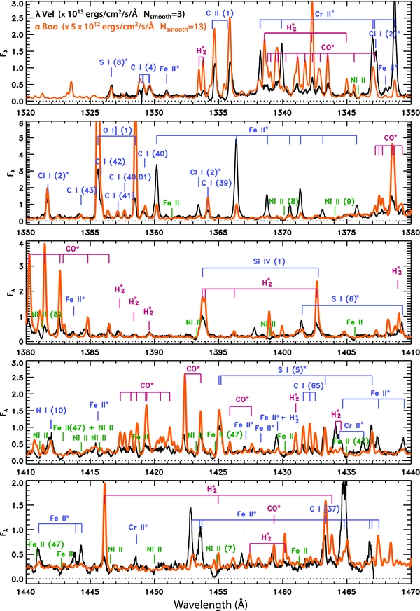
Figure 3. Comparison of the COS λ Vel spectrum with a STIS observation of α Boo. The α Boo spectrum has been scaled to approximately match the continua of the two stars. CO and O i fluorescent lines are strong in both spectra. The absorption features and Fe ii fluorescent emission lines seen in λ Vel are weak or absent in α Boo. See the caption to Figure 1 for more information on the labels.
Download figure:
Standard image High-resolution image
Figure 4. Comparison of the COS λ Vel spectrum with a STIS observation of α Ori. Lambda Vel has a similarly strong far-ultraviolet continuum, but CO lines in emission rather than in absorption. The λ Vel spectrum has clear H2 and strong Fe ii fluorescent emissions. The C ii (UV 1) doublet near 1335 Å, the Si iv (UV 1) doublet at 1400 Å, and the Cl i fluorescent feature near 1352 Å are much stronger in the early-K supergiant than in α Ori. The atomic absorptions of Fe ii and Ni ii, while seen in both stars, are significantly broader in λ Vel, suggesting a higher turbulence in the K supergiant wind. See the caption to Figure 1 for more information on the labels.
Download figure:
Standard image High-resolution imageAlpha Boo and λ Vel have similar effective temperatures, but α Boo has a considerably higher surface gravity and therefore a less-extended, denser outer atmosphere (see Section 2 and Table 1). Figure 3 compares the COS λ Vel spectrum with a STIS spectrum of α Boo from StarCAT (Ayres 2010), a catalog of high-resolution ultraviolet (UV) spectra of objects classified as "stars," recorded by Space Telescope Imaging Spectrograph (STIS) during its initial seven years of operations (1997–2004).
Lambda Vel and α Ori have low surface gravities and extended outer atmospheres, but α Ori has a cooler effective temperature and a more massive wind, as well as thick circumstellar shells not observed around λ Vel. The definitive far-ultraviolet observation of α Ori until recently was a low-resolution GHRS G140L spectrum (Carpenter et al. 1994), which enabled an initial understanding of this spectral region in the M supergiant as it made clear the existence of a strong far-ultraviolet chromospheric continuum over which a series of strong molecular absorption bands of carbon monoxide from its circumstellar shells was superposed. In α Ori, the chromospheric emission lines characteristics of cool stars are seen superposed on a continuum that is modified by absorption and re-emission in the CO bands. Recently, the ASTRAL: Cool Stars Program (GO 12278) obtained a high-resolution set of STIS observations of α Ori, including this region, which reveals the finer details (Carpenter et al. 2013; Nielsen et al. 2013). Figure 4 compares the COS λ Vel spectrum with the high-resolution STIS ASTRAL spectrum of α Ori.
The various components of the λ Vel spectrum are discussed in the subsequent sections. Line identifications have been made using the Kurucz databases6 (Kurucz 1995, 2005) with reference to the NIST Atomic Line Database7 and the Ultraviolet Multiplet Tables (Moore 1983 and preceding), the Arcturus UV Spectral Atlas (Hinkle et al. 2005), the IUE studies of Arcturus described in Ayres (1986), Ayres et al. (1986), and the GHRS studies of λ Vel (Carpenter et al. 1999). In addition to wavelength coincidence, we checked to make sure that all of the expected lines, based on intrinsic line strength (e.g., gf value), from a given energy level (lower if absorption, upper if emission) were seen if in the wavelength range of the observation. For the emission lines characterized as fluorescent, we also required that the exciting line and the excitation route be identified for the ID to be considered solid. Lines and excited levels above those populated in plasma with a temperature 20,000 K or lower were not considered unless a radiative excitation process was found to populate the level.
3.1. The Far-ultraviolet Continuum
The strong far-ultraviolet continuum observed in λ Vel is brighter than expected from the photosphere of a K supergiant. The upper panel of Figure 5 compares the observed surface fluxes of λ Vel with two synthetic continua computed with ATLAS9 (Kurucz 1993): one standard model and one in which a temperature minimum (Tmin/Teff = 0.8) is enforced for the uppermost layers. The optical data of Kiehling (1987) are well-matched by the models, but the observed ultraviolet continuum is more than two orders of magnitude above the synthetic spectrum at 2700 Å and more than six orders of magnitude at 1800 Å. The model with the flat temperature minimum matches the observed flux distribution to shorter wavelengths, but even this model falls well below the observations shortward of 2000 Å, implying the presence of a temperature rise above the photosphere. We have further characterized this temperature rise by computing the mean effective radiation temperature corresponding to the observed flux, from the optical down into the far-UV range covered by the COS and GHRS, by setting the surface flux at a given wavelength to πB (where B is the Planck function) and then solving for the corresponding temperature. The lower panel of Figure 5 shows this effective radiation temperature versus wavelength. This confirms the Tmin of about 3200 K derived above using the modified Kurucz models and shows the chromospheric temperature rise as one looks to progressively shorter wavelengths, and thus higher altitudes, than included in the modified Kurucz model. The temperature at the longer wavelengths approximates, as expected, the effective temperature of the stellar photosphere. The observed ultraviolet continuum thus must form at chromospheric altitudes. Evidence of a chromospheric continuum in λ Vel was reported by Carpenter et al. (1999) using GHRS data. However, the GHRS wavelength coverage was mainly longward of 1800 Å, with one solitary observation near 1300 Å. The COS spectrum partly fills the gap in the GHRS sampling and confirms the extension of the bright continuum into far-ultraviolet wavelengths.

Figure 5. Top: comparison of the observed continuum surface flux distribution of λ Vel with two Kurucz synthetic continua. Observed data are from Kiehling (1987) (optical), HST/GHRS, and HST/COS, while the synthetic continua were computed with a standard Kurucz model and one in which a minimum temperature was enforced throughout the upper layers. Orders of magnitude separate the observed UV from the photospheric models; clear evidence of continuum emission from the hotter chromospheric layers. The new COS data confirm the far-UV excess seen in earlier GHRS measurements. Bottom: the chromospheric temperature rise implied by the observed fluxes is shown in this plot of the effective radiation temperature vs. wavelength.
Download figure:
Standard image High-resolution imageThe observed chromospheric continuum emission of λ Vel is reminiscent of the continuum observed in α Ori (Carpenter et al. 1994). However, the absence of the strong circumstellar absorption in the CO absorption bands seen in α Ori, makes the chromospheric continuum in λ Vel more uniform. Alpha Boo (K1.5 III), in contrast, shows a weaker far-ultraviolet continuum. This is consistent with the two supergiants having a greater mass column density (mcol) in their chromospheres than the giant stars, which shifts optical depth unity surfaces to larger radii in the supergiants in accordance with the scaling relation from Ayres (1979): mcol(τ)∝g−0.5. The temperature of the chromosphere is increasing with height and the continuum flux rises (as the Planck function in the UV is very sensitive to the temperature) as one goes higher in the chromosphere. The chromospheric continuum in λ Vel, as in α Ori, is larger than in the giant star because the optical depth unity surface is at a greater radius and thus presents both a higher temperature and a larger emitting surface.
3.2. The Line Emission Spectrum
Fluorescent processes are common in cool, evolved stars. Ayres (1986) and Ayres et al. (2001) examined IUE and GHRS spectra of α Boo and Carpenter et al. (1988) studied IUE spectra of γ Cru (M3.4 III) to identify and catalog the radiative pumping processes and products observed at far- and near-ultraviolet wavelengths. Subsequent papers will exploit the more extensive ASTRAL STIS spectra of α Ori and γ Cru.
The line emission spectrum in λ Vel is dominated by fluorescent features from both atomic and molecular species. Atomic fluorescence is identified in O i, S i, Cl i, Cr ii, and especially Fe ii, while molecular fluorescence is detected in CO and H2.
The main source of excitation for these fluorescent processes is H i Lyα, whose broad and intense emission profile coincides with a large number of transitions that can serve as pumping channels. This is evident in particular in Cr ii and Fe ii, both of which show a strong primary fluorescent spectrum. The hot chromosphere provides an environment to collisionally populate energy states up to 20,000 cm−1 in Cr ii and Fe ii. With strong H i Lyα radiative pumping, these states can be excited to above 90,000 cm−1, from which the decays produce a large number of fluorescent lines longward of H i Lyα. By a similar process as for Fe ii and Cr ii, molecular hydrogen is pumped from an excited vibrational level in its ground electronic state, producing the Lyman band emission spectrum shortward of 1650 Å.
Besides H i Lyα induced fluorescence, other processes fed by O i and C ii are observed in CO and Cl i, respectively. The CO spectrum is highly dependent on the presence of prominent O i triplet emission λλ1302, 1304, 1306. The oxygen O i] λ1355 line is prominent in the λ Vel spectrum, which might be due to fluorescence fed by H i Ly β, consistent with a strong oxygen triplet emission.
The ability of any line to serve as a fluorescent pump depends both on its strength as well as its width, and the latter depends on the surface gravity and generally increases with decreasing surface gravity. More specifically, it is the mean intensity at the exciting frequency summed over the whole atmosphere that is crucial to the pumping efficiency and it does not have a one-to-one equivalence to the observed flux profile, especially as that profile may be distorted by circumstellar and/or interstellar absorption. Consequently, the observed-at-Earth fluxes and profiles of the pumps such as H i Lyβ (as may have been observed by the Far-Ultraviolet Spectroscopic Explorer, FUSE, for example) are not necessarily informative regarding the suitability of the line as a pump, as the chromospheric line strength and profile can differ dramatically from that observed from Earth. For further discussion of H i Lyα fluorescence processes and their dependence on, and what they tell us about, the H i Lyα profile, see Harper et al. (2001), Wood & Karovska (2004), and Herczeg et al. (2006).
The H i Lyα radiation also is responsible for the prominent S i fluorescence spectrum. In cooler M stars and higher gravity K stars, S i emission in UV 9 has been attributed to O i pumping (Brown & Jordan 1980). In λ Vel, the S i spectrum is more dominant with many more of the higher levels of S i populated. The ionization potential for neutral sulfur is close to the H i Lyα transition energy, and consequently the H i spectrum can populate the numerous high lying levels close to the ionization limit. The resulting cascades produce the observed prominent S i spectrum in late-type giant stars (Tondello 1972; Judge 1988), including the strong multiplets (UV 5, 6, 8) observed at COS wavelengths.
The molecular fluorescence is, as seen in Figure 3, weaker in λ Vel than in the K1.5 III giant α Boo. The H2 lines are pumped exclusively by H i Lyα, while the CO lines are primarily pumped by the O i (UV 2) lines (which in turn are pumped by Lyβ) with smaller contributions from H i Lyα and the C i resonance multiplet at 1657 Å. In contrast, the Fe ii and Cr ii fluorescent lines, which are also pumped by H i Lyα, are much stronger in λ Vel. The weakness of the molecular fluorescence in λ Vel relative to that in α Boo indicates that the H i pumps are weaker in λ Vel than in α Boo. The strength of the Fe ii and Cr ii fluorescent lines in λ Vel, relative to that seen in α Boo, thus cannot be due to a stronger exciting flux from H i in λ Vel, but is instead likely due to the higher abundance of the iron group elements in λ Vel, as noted in Table 1, which reflects values derived by Ramírez & Allende Prieto of [Fe/H] = −0.52 for α Boo compared to [Fe/H] = +0.23 for λ Vel, a difference of 0.75 dex.
The λ Vel spectrum exhibits similarly strong fluorescent Fe ii emission as that observed in evolved M stars, such as α Ori (Figure 4). The narrow CO emission features seen throughout this wavelength region in λ Vel are, however, less prevalent in the M supergiant due to the presence of strong circumstellar CO (A-X) absorption bands that mask a number of those features in the α Ori spectrum. CO fluorescent emission is seen in α Ori outside these bands, for example, in the region between 1375–1386 Å, as well as fluorescent H2 emission. The Fe ii lines near 1368–1374 Å are weak in α Ori, and are likely absorbed higher in the atmosphere by the circumstellar CO bands since other transitions from the same upper energy levels are prominent. The C ii (UV 1) doublet near 1335 Å, the Si iv (UV 1) doublet near 1400 Å, and the Cl i fluorescent feature near 1352 Å are much stronger in the early-K supergiant than in α Ori (in fact, the Si iv (UV 1) doublet is not seen at all in α Ori).
The Cl i fluorescence usually is restricted to the single line Cl i λ1351 (Shine 1983). Its upper level (4s 2P1/2) can be populated by Cl i λ1335, which overlaps with a chromospheric C ii λ1335. The other transitions in Cl i UV 2 (at 1347 and 1363 Å) cannot easily benefit from the C ii pump and consequently are absent in spectra of cool evolved stars such as α Boo (see Figure 4). In α Ori, the entire Cl i UV 2 multiplet is missing. Lines from Cl i λλ1379, 1398, 1996 (UV 1) are not present in λ Vel, α Ori, or α Boo. This is, in part, explained by their lower transition probabilities and collisional cross sections.
In λ Vel all three lines of Cl i UV 2 are present, but the population mechanism for the upper state of Cl i λλ1347,1363 (4s 2P3/2) is uncertain. There is no clear second pump for the J = 3/2 level, although the width and strength of either Cr ii λ1347 or C ii λ1335 provide a means to populate 4s 2P3/2. There is a coincidence between Cl i λ1347 and the strong Cr ii λλ1347.035, 1347.167 fluorescent lines, both pumped by H i Lyα; and the Cl i λ1347 line could be populating the J = 3/2 level via radiative pumping in the wing of the Cr ii blend. Cl i λ1347 is not seen in absorption against the Cr ii line, but this is expected if the Cr ii line is much stronger than the Cl i; also, the Cl i line might be mostly absorbing Cr ii photons emitted downward, or laterally, in the lower chromosphere. Alternatively, the C ii pumping of the J = 1/2 level could be so intense that collisional redistribution to J = 3/2 is sufficient to produce the Cl i λλ1347, 1363 emission.
The spectrum displays a modest number of non-fluorescent atomic emission lines. Collisionally excited levels are observed in C i and C ii, especially the strong C ii resonance features near 1335 Å (UV 1). The Si iv λλ1394,1403 (UV 1) likely suffer substantial contamination by H2 fluorescent emission, as seen in α Boo (Ayres et al. 2003). The Si iv lines are present at some degree and thus are evidence for the existence of hot material (∼8 × 10⁴ K) in the supergiant's outer atmosphere. This hot material must somehow coexist with the cool wind (absorbing strongly in the lower temperature C ii resonance lines).
The prominent emission line near 1412 Å is tentatively identified as N i (UV 10). This transition has an upper level close to 100,000 cm−1 that is difficult to populate at typical chromospheric temperatures. We are unable to find a suitable radiative pump so its presence is currently unconfirmed. However, this line is commonly identified in giant stars, especially in the post-flash clump giants where the nitrogen abundance often is significantly enhanced. If the nitrogen abundance is dramatically elevated this may enable adequate population of that high level even at moderate temperatures.
3.3. The Absorption Spectrum
Multiple absorption features, including strong Fe ii and Ni ii, are seen against the chromospheric continuum of λ Vel. The strong Fe ii and Ni ii absorptions seen in the λ Vel spectrum are weaker or non-existent in α Boo, which also would be consistent with the lower iron-group abundance in α Boo, as well as the expected lower column densities in the wind from the giant star. These lines are seen in α Ori, but they are narrower than in λ Vel, suggesting a higher turbulence in the chromosphere and wind of the K supergiant.
There is no evidence of the CO (A-X) absorption bands that dominate the far-UV spectrum of α Ori in the λ Vel spectrum.
4. SPECTRAL LINE ANALYSIS
We have measured the wavelengths and integrated fluxes of all identified emission features in the COS spectrum and list them in Tables 2 (atomic species) and 3 (molecules). A linear fit is used to quantify the local continuum around and under the emission features so that the continuum could be subtracted from the measurements. The measurements are thus of the net integrated line flux. The line centers and FWHMs were determined by fitting one or more Gaussians to each feature, a single Gaussian to clean, unblended lines and multiple Gaussians in the case of blends. We used the FUSE IDL procedure XGAUSSFIT8 to obtain these measurements and intrinsic IDL function GAUSSFIT to estimate the standard errors of those values. The velocity measurements of the emission lines have a mean standard error of 1.03 km s−1, which reflects the accuracy of our ability to fit a line in this data set and is a good estimate of the errors in our relative velocity measurements of individual lines. As noted earlier, the absolute values are more uncertain due to the large COS science aperture, which limits the precision of the absolute velocities to ∼15 km s−1, although relative velocities of groups of lines can be measured to much higher precision by computing means over large sets of lines and/or comparing histograms of the measured velocities of the various groups. Formally, mean velocities of groups of lines have smaller errors by a factor of 1/ , where N = number of lines in the set. However, we choose to compare the distributions of the measured velocities of the different sets of lines by fitting Gaussians to their histograms and comparing the centroids of those fits to best determine their mean relative velocity. The standard errors in the measurements of the FWHM and net integrated flux of each line vary more from line to line, depending on the line strength, but the mean standard errors of the two are ∼2.7 km s−1 and ∼2.0 × 10⁻¹⁵ erg cm−2 s−1, respectively.
Table 2. Properties of Atomic Emission Lines in the COS λ Vel Spectrum
| λlab | ID | RV | FWHM | Integ. Flux (×10−15) | Fsurf |
|---|---|---|---|---|---|
| (Å) | (km s−1) | (km s−1) | (erg cm−2 s−1) | (erg cm−2 s−1) | |
| 1326.642 | S i (UV 8)** | −3.9 | 56 | 7.7 | 17.7 |
| 1328.834 | C i (UV 4) | −7.2 | 45 | 3.8 | 8.8 |
| 1329.085 | C i (UV 4) | 17.3 | 40 | 5.9 | 13.5 |
| 1329.577 | C i (UV 4) | 11.1 | 72 | 9.1 | 20.9 |
| 1330.952 | Fe ii* | −3.6 | 45 | 3.7 | 8.6 |
| 1334.532 | C ii (UV 1) | 41.8 | 62 | 34.9 | 80.4 |
| 1335.708 | C ii (UV 1) | 46.0 | 71 | 36.8 | 84.8 |
| 1338.237 | Cr ii* | 1.1 | 57 | 32.2 | 74.0 |
| 1339.904 | Cr ii* | 3.8 | 49 | 34.8 | 79.9 |
| 1346.189 | Fe ii* | 13.9 | 32 | 1.0 | 2.3 |
| 1347.035 | Cr ii* | −8.4 | 55 | 44.0 | 100.7 |
| 1347.240 | Cl i (UV 2) | 8.6 | 56 | 32.1 | 73.4 |
| 1348.006 | Fe ii* | 2.9 | 55 | 5.0 | 11.5 |
| 1348.724 | Cr ii* | 2.5 | 58 | 82.4 | 188.4 |
| 1351.297 | Cr ii* | −0.3 | 67 | 6.1 | 14.0 |
| 1351.656 | Cl i (UV 2)*** | 4.8 | 59 | 31.2 | 71.1 |
| 1352.572 | Cr ii* | 0.9 | 58 | 5.3 | 12.0 |
| 1352.988 | C i (43.01) | 8.5 | 31 | 1.7 | 3.9 |
| 1354.288 | C i (UV 43) | −28.5 | 65 | 7.1 | 16.1 |
| 1355.598 | O i (UV 1) | 0.0 | 57 | 79.6 | 181.6 |
| 1355.844 | C i (UV 42) | 13.4 | 50 | 17.9 | 40.7 |
| 1357.134 | C i (UV 41) | 2.7 | 34 | 2.3 | 5.2 |
| 1357.659 | C i (UV 40.01) | −1.1 | 23 | 2.0 | 4.5 |
| 1358.512 | O i (UV 1) | −3.8 | 43 | 23.7 | 53.9 |
| 1359.061 | Fe ii* | −3.1 | 31 | 3.5 | 8.0 |
| 1359.275 | C i (UV 40) | −11.3 | 49 | 6.0 | 13.7 |
| 1360.178 | Fe ii* | 1.6 | 56 | 80.0 | 181.9 |
| 1363.448 | Cl i (UV 2) | 0.6 | 53 | 18.9 | 43.0 |
| 1364.164 | C i (UV 39) | −0.4 | 46 | 10.0 | 22.7 |
| 1365.038 | Cr ii* | −3.6 | 44 | 2.8 | 6.5 |
| 1366.394 | Fe ii* | −1.0 | 57 | 127.2 | 288.6 |
| 1368.807 | Fe ii* | −3.0 | 50 | 32.5 | 73.6 |
| 1370.532 | Fe ii* | 10.4 | 44 | 16.9 | 38.2 |
| 1371.390 | Fe ii* | −1.5 | 53 | 42.7 | 96.7 |
| 1373.122 | Fe ii* | −1.3 | 46 | 10.2 | 23.1 |
| 1379.713 | Fe ii* | −7.7 | 70 | 13.5 | 30.5 |
| 1383.714 | Fe ii* | −7.6 | 41 | 2.9 | 6.5 |
| 1393.755 | Si iv (UV 1) | 5.8 | 112 | 43.2 | 96.8 |
| 1401.514 | S i (UV 6)** | −0.6 | 64 | 16.2 | 36.3 |
| 1402.770 | Si iv (UV 1) | 21.0 | 47 | 5.8 | 13.0 |
| 1409.127 | Fe ii* | −18.1 | 31 | 3.9 | 8.7 |
| 1409.337 | S i (UV 6)** | −2.4 | 48 | 11.8 | 26.2 |
| 1411.931 | N i (UV 10) | −19.3 | 65 | 13.4 | 29.9 |
| 1415.572 | Fe ii* | −12.7 | 51 | 6.8 | 15.2 |
| 1423.691 | Fe ii* | 22.1 | 53 | 7.2 | 16.1 |
| 1425.030 | S i (UV 5)** | 4.2 | 55 | 19.6 | 43.6 |
| 1425.188 | S i (UV 5)** | 15.4 | 46 | 12.9 | 28.6 |
| 1427.133 | Fe ii* | −6.1 | 46 | 3.8 | 8.4 |
| 1429.592 | Fe ii* | 1.1 | 56 | 14.4 | 31.9 |
| 1431.596 | C i (UV 65) | 3.4 | 36 | 4.8 | 10.7 |
| 1432.105 | C i (UV 65) | 9.6 | 40 | 3.5 | 7.8 |
| 1432.529 | C i (UV 65) | 17.2 | 59 | 3.4 | 7.6 |
| 1433.278 | S i (UV 5)** | 9.4 | 57 | 21.6 | 47.8 |
| 1434.401 | Cr ii* | 6.6 | 33 | 5.9 | 13.0 |
| 1434.669 | Fe ii* | −7.2 | 43 | 7.9 | 17.4 |
| 1436.316 | Cr ii* | 2.7 | 52 | 10.8 | 23.9 |
| 1436.967 | S i (UV 5)** | 3.1 | 52 | 21.0 | 46.5 |
| 1437.457 | Fe ii* | −1.5 | 60 | 13.6 | 30.0 |
| 1439.469 | Fe ii* | −0.6 | 54 | 11.4 | 25.2 |
| 1440.988 | Fe ii* | −1.8 | 42 | 6.1 | 13.4 |
| 1443.866 | Fe ii* | −5.2 | 65 | 8.2 | 18.1 |
| 1444.296 | S i** | 17.2 | 52 | 10.6 | 23.4 |
| 1448.614 | Cr ii* | 2.5 | 34 | 3.6 | 7.8 |
| 1452.923 | Fe ii* | −0.2 | 53 | 32.6 | 71.7 |
| 1453.509 | Fe ii* | −6.4 | 81 | 9.5 | 20.9 |
| 1453.702 | Fe ii* | −1.3 | 53 | 18.3 | 40.2 |
| 1463.336 | C i (UV 37) | 1.3 | 63 | 20.6 | 45.2 |
| 1464.782 | Fe ii* | 2.6 | 41 | 29.5 | 64.6 |
| 1464.983 | Fe ii* | 4.0 | 42 | 36.8 | 80.7 |
| 1466.954 | Fe ii* | −15.4 | 30 | 6.6 | 14.5 |
Notes. Velocities are all relative to the stellar radial velocity of 17.6 km s−1 (Gontcharov 2006). *Primary fluorescence pumped by H i Lyα. **Cascade fluorescence pumped by H i Lyα. ***Primary fluorescence pumped by C ii λ1335.
Table 3. Properties of Molecular Emission Lines in the COS λ Vel Spectrum
| λlab | ID | RV | FWHM | Integ. Flux (×10−15) | Fsurf |
|---|---|---|---|---|---|
| (Å) | (km s−1) | (km s−1) | (erg cm−2 s−1) | (erg cm−2 s−1) | |
| 1333.797 | H2 0−4 R1 | 3.1 | 49 | 3.2 | 7.4 |
| 1338.568 | H2 0−4 P2 | 9.0 | 43 | 5.1 | 11.8 |
| 1338.816 | CO 11−2 R21 | −4.3 | 37 | 4.6 | 10.5 |
| 1339.059 | CO 11−2 Q19 | −4.7 | 42 | 2.5 | 5.8 |
| 1339.460 | CO 9−1 Q8 | 0.0 | 40 | 5.9 | 13.5 |
| 1339.626 | CO 9−1 Q9 | 5.4 | 42 | 6.8 | 15.7 |
| 1340.236 | CO 9−1 Q12 | −4.4 | 53 | 4.1 | 9.4 |
| 1341.171 | CO 13−3 Q26 | −9.0 | 42 | 5.9 | 13.6 |
| 1341.435 | CO 9−1 P14 | −1.7 | 41 | 1.3 | 3.0 |
| 1341.726 | CO 11−2 Q25 | 5.8 | 40 | 2.4 | 5.5 |
| 1342.256 | H2 0−4 P3 | 9.8 | 51 | 11.3 | 25.9 |
| 1342.923 | CO 11−2 P25 | −14.0 | 83 | 9.1 | 20.9 |
| 1343.486 | CO 9−1 Q22 | 9.4 | 51 | 8.6 | 19.7 |
| 1345.065 | CO 9−1 P23 | −3.8 | 38 | 1.7 | 3.9 |
| 1345.563 | CO 9−1 P24 | −10.0 | 28 | 1.2 | 2.8 |
| 1359.082 | H2 4−6 R3 | −7.7 | 31 | 3.5 | 8.0 |
| 1377.210 | CO 11−3 R21 | −20.7 | 58 | 8.6 | 19.4 |
| 1377.494 | CO 11−3 Q19 | 8.3 | 49 | 5.9 | 13.4 |
| 1377.767 | CO 9−2 R4 | −0.9 | 38 | 7.9 | 17.9 |
| 1378.019 | CO 11−3 R23 | −4.1 | 43 | 5.5 | 12.5 |
| 1378.522 | CO 9−2 Q8 | −0.7 | 26 | 8.4 | 18.9 |
| 1378.693 | CO 9−2 Q9 | −2.3 | 42 | 16.6 | 37.4 |
| 1379.317 | CO 9−2 Q12 | −12.9 | 52 | 11.4 | 25.7 |
| 1379.721 | H2 3−4 R16 | −9.4 | 70 | 13.5 | 30.5 |
| 1380.093 | H2 1−4 P11 | −6.8 | 39 | 9.6 | 21.8 |
| 1380.250 | CO 9−2 P13 | −9.3 | 26 | 6.0 | 13.6 |
| 1380.399 | CO 11−3 P23 | −16.5 | 43 | 8.5 | 19.2 |
| 1381.442 | CO 9−2 Q19 | 3.3 | 50 | 10.4 | 23.4 |
| 1382.642 | CO 9−2 Q22 | −7.5 | 34 | 13.4 | 30.1 |
| 1382.881 | CO 9−2 P20 | −4.5 | 30 | 4.5 | 10.1 |
| 1384.811 | CO 9−2 P24 | −4.9 | 22 | 2.1 | 4.8 |
| 1386.462 | CO 9−2 P27 | −6.1 | 33 | 5.5 | 12.4 |
| 1387.362 | H2 1−5 P5 | −30.2 | 63 | 6.2 | 14.0 |
| 1389.584 | H2 0−4 R11 | 14.4 | 66 | 5.2 | 11.6 |
| 1402.648 | H2 0−5 P3 | 3.1 | 73 | 17.2 | 38.4 |
| 1409.024 | H2 1−5 P8 | 3.8 | 31 | 3.9 | 8.7 |
| 1417.342 | CO 11−4 R21 | −6.7 | 52 | 5.2 | 11.7 |
| 1418.167 | CO 11−4 R23 | 2.2 | 59 | 4.5 | 10.1 |
| 1418.617 | CO 9−3 R4 | 2.6 | 46 | 6.0 | 13.3 |
| 1419.309 | CO 9−3 R11 | −16.2 | 15 | 0.9 | 2.1 |
| 1419.400 | CO 9−3 Q8 | −9.4 | 55 | 4.5 | 10.1 |
| 1419.574 | CO 9−3 Q9 | 3.7 | 17 | 0.8 | 1.8 |
| 1420.953 | CO 9−3 R18 | −3.5 | 42 | 3.4 | 7.5 |
| 1421.193 | CO 9−3 P13 | −2.7 | 27 | 1.9 | 4.1 |
| 1422.386 | CO 9−3 Q19 | −6.0 | 41 | 9.5 | 21.0 |
| 1423.614 | CO 9−3 Q22 | −4.0 | 41 | 10.6 | 23.4 |
| 1425.879 | CO 9−3 P24 | −6.8 | 31 | 2.1 | 4.6 |
| 1431.010 | H2 1−6 R3 | 1.2 | 42 | 1.5 | 3.2 |
| 1434.097 | H2 3−7 R2 | 18.0 | 61 | 24.6 | 54.5 |
| 1446.118 | H2 1−6 P5 | 4.2 | 68 | 7.1 | 15.7 |
| 1457.435 | H2 0−6 P1 | −6.7 | 21 | 1.6 | 3.5 |
| 1459.323 | CO 11−5 R21 | −7.1 | 37 | 4.9 | 10.8 |
| 1460.165 | H2 0−6 P2 | 0.2 | 21 | 1.2 | 2.7 |
| 1463.826 | H2 0−6 P3 | 8.3 | 62 | 4.8 | 10.5 |
| 1467.079 | H2 1−6 P8 | −19.3 | 10 | 1.3 | 2.8 |
Notes. Velocities are all relative to the stellar radial velocity of 17.6 km s−1 (Gontcharov 2006). All H2 and CO lines are pumped by H i Lyα and the O i λ1300 triplet, respectively.
Download table as: ASCIITypeset image
Identifications and measurements of the prominent atomic absorption features are presented in Table 4. These absorption features were also fit with Gaussians, relative to the local continuum, as done for the emission features and with similar accuracy.
Table 4. Properties of Absorption Lines in the COS λ Vel Spectrum
| λlab | ID | Elow | RV | FWHM | Wλ |
|---|---|---|---|---|---|
| (Å) | (cm−1) | (km s−1) | (km s−1) | (Å) | |
| 1334.532 | C ii | 0 | 12.8 | 127 | 0.92 |
| 1335.201 | Ni ii | 1507 | −12.5 | 42 | 0.09 |
| 1335.708 | C ii | 63 | −14.8 | 123 | 0.69 |
| 1345.878 | Ni ii | 0 | −9.4 | 67 | 0.21 |
| 1361.373 | Fe ii | 13474 | −13.0 | 62 | 0.18 |
| 1368.094 | Fe ii | 13673 | −28.5 | 73 | 0.18 |
| 1370.132 | Ni ii (UV 8) | 0 | −25.7 | 85 | 0.38 |
| 1374.072 | Ni ii (UV 9) | 1507 | −14.1 | 88 | 0.30 |
| 1381.286 | Ni ii (UV 8) | 1507 | 1.4 | 47 | 0.17 |
| 1393.324 | Ni ii | 0 | −10.3 | 79 | 0.33 |
| 1399.018 | Ni ii | 1507 | −11.5 | 100 | 0.26 |
| 1404.119 | Fe ii | 1873 | −3.1 | 113 | 0.17 |
| 1405.608 | Fe ii | 1873 | −18.8 | 83 | 0.30 |
| 1411.065 | Ni ii | 1507 | −11.8 | 69 | 0.25 |
| 1412.842 | Fe ii (UV 47) | 1873 | −15.8 | 94 | 0.41 |
| 1414.292 | Ni ii | 0 | −2.0 | 87 | 0.23 |
| 1415.720 | Ni ii | 0 | 4.3 | 78 | 0.22 |
| 1416.711 | Fe ii | 2430 | −5.0 | 47 | 0.12 |
| 1418.853 | Fe ii | 1873 | −8.1 | 105 | 0.35 |
| 1423.206 | Ni ii | 1507 | −2.0 | 50 | 0.13 |
| 1424.717 | Fe ii (UV 47) | 2430 | −12.8 | 86 | 0.36 |
| 1430.167 | Fe ii | 2430 | −4.9 | 83 | 0.17 |
| 1433.044 | Fe ii | 2838 | −1.4 | 41 | 0.08 |
| 1434.996 | Fe ii (UV 47) | 2838 | 0.9 | 68 | 0.22 |
| 1438.133 | Fe ii | 2430 | −4.6 | 36 | 0.05 |
| 1440.775 | Fe ii (UV 47) | 3117 | −1.9 | 65 | 0.19 |
| 1442.746 | Fe ii | 3117 | −3.6 | 54 | 0.16 |
| 1444.981 | Fe ii | 2838 | 1.5 | 59 | 20.17 |
| 1446.581 | Ni ii | 1507 | −7.0 | 65 | 0.17 |
| 1447.272 | Fe ii | 3117 | −3.7 | 52 | 0.08 |
| 1448.011 | Co ii | 0 | −3.8 | 58 | 0.06 |
| 1449.997 | Ni ii | 0 | −6.0 | 76 | 0.17 |
| 1454.842 | Ni ii (UV 7) | 0 | −19.0 | 79 | 0.36 |
| 1455.231 | Fe ii | 385 | −22.8 | 107 | 0.14 |
| 1455.885 | Co ii | 951 | −14.1 | 43 | 0.06 |
| 1461.247 | Fe ii | 668 | −15.2 | 101 | 0.17 |
| 1465.421 | Fe ii | 863 | 22.2 | 10 | 0.02 |
Notes. Velocities are all relative to the stellar radial velocity of 17.6 km s−1 (Gontcharov 2006).
Download table as: ASCIITypeset image
The apparent velocities of all the features are relative to the stellar photospheric radial velocity of 17.6 ± 0.3 km s−1 (Gontcharov 2006), which we note is 0.4 km s−1 smaller than used in the original Carpenter et al. (1999) λ Vel study. However, the radial velocities were corrected for the instrumental systematic trend discussed in Section 2, a process that results in the mean velocity of the chromospheric (atomic) emission lines (excluding the wind-impacted C ii and Si iv lines) being set to zero. The angular diameter used to compute the surface fluxes is 11.1 mas (Blackwell & Shallis 1977).
The distributions of the measured velocities for the atomic absorption and emission features are shown in the top panel of Figure 6, while the histograms of the measured velocities of the molecular emission and atomic emission features are given in the lower panel. We note that heavily blended features or features contaminated by overlying wind absorption, e.g., C ii and Si iv near 1335 Å and 1400 Å, are excluded from these samples. It appears that the atomic emission and absorption features belong to two different distributions, with the absorption components blueshifted relative to the emission spectrum by 7.6 km s−1, implying formation in the lower levels of the outflowing wind. The histogram of the RV's of the molecular CO and H2 emission features define a third population and appear to be blueshifted by 3.3 km s−1relative to the atomic emission features, suggesting formation slightly above the chromospheric regions, in the lowest levels of the outflowing wind, and below the region in which the atomic absorption lines are formed. These values are all well below the terminal velocity of the wind reported by Carpenter et al. (1999) from earlier GHRS data and estimated below from the current COS data set by modeling the C ii P Cyg lines. In order to confirm these conclusions, we have performed a two-sample Kolmogorov–Smirnov (K-S) test on the two pairs of distributions to assess whether: (1) the "Atomic Emission" and "Atomic Absorption" line velocity distributions are from the same or different parent distributions and (2) the atomic and molecular emission line velocity distributions are from the same or different parent distributions. The K-S test run on the first pair gives K-S statistic of 0.404 and a probability of the two distributions being from the same parent distribution as 0.00083, indicating the two are indeed distinct and the velocity difference is meaningful. Similarly, a K-S test on the second pair gives a K-S statistic of 0.617 and a probability of the two distributions being from the same parent as 0.00008, again indicating the two distributions are from different parents and that the velocity difference is meaningful. In both the histograms and the K-S tests, we used the 38 cleanest (unblended, good S/N, uncontaminated by overlying wind absorption) atomic emissions lines, all 55 molecular emission lines, and the 18 cleanest atomic absorption lines.

Figure 6. Top: histograms of the measured velocities of the chromospheric emission (red) and wind absorption (blue) lines. The measurements clearly indicate two different populations with the absorption lines on average blueshifted by ∼7.6 km s−1 relative to the emission lines, reflecting formation in the outflowing stellar wind. Bottom: histograms of the measured velocities of the chromospheric atomic (red) and molecular (green) emission lines. The two sets of lines again are seen to belong to different populations, with the molecular emission lines blueshifted by ∼3.3 km s−1 relative to the atomic emission features, suggesting they form in the region near the base of the wind acceleration, above the mean height of the atomic emission but below that of the atomic absorption features.
Download figure:
Standard image High-resolution image5. INFERRED PROPERTIES OF THE CHROMOSPHERE AND STELLAR WIND
We have used the new COS spectrum, with reference to the archival GHRS spectra, to improve our characterization of the properties of the chromospheric regions and wind of λ Vel. The influence of the stellar wind is seen most clearly in the P Cygni profiles of C ii λλ1334,1335, in the blueshifted Fe ii and Ni ii wind absorption lines in the COS spectrum, and in the self-reversed Fe ii profiles in the near ultraviolet GHRS data. The wind lines studied previously indicate a turbulent velocity that varies with height and ranges from 9–21 km s−1 and a terminal wind speed of ∼30 km s−1 (Carpenter et al. 1999).
The presence of hot plasma in the atmosphere of the star, indicated by previous GHRS observations of Si iii] and C iii] lines at 1900 Å (Carpenter et al. 1999) and FUSE observations of O vi λ1032 Harper et al. (2005), is confirmed by the detection of Si iv λλ1398,1403 in this COS spectrum implying a plasma temperature of ∼8 × 10⁴ K. Both components of the doublet are contaminated by fluorescent H2 emission making it difficult to measure a reliable flux for this doublet. The suggestion by Ayres (1986) that hot and cold material are intermingled in the chromosphere is supported by the fluorescent molecular lines visible throughout the λ Vel ultraviolet spectrum. Harper et al. (2005) argue that the presence of O vi must indicate magnetic heating, as acoustic heating of significant amounts of material up to 300,000 K is extremely difficult to achieve. We note that Grunhut et al. (2010) reported a 5σ magnetic field measurement for λ Vel, 〈Bz〉 = 1.72 ± 0.33 G.
We have made approximate, Sobolev with Exact Integration (SEI) fits (Lamers et al. 1987) to C ii λλ1334, 1335 (Figure 7) to derive the wind parameters, as demonstrated by Carpenter et al. (1999) using GHRS observations. The C ii line 1335 Å comprises of two albeit unequal lines, so C ii λ1334 is preferred for modeling purposes to estimate wind parameters that are comparable with the results from Carpenter et al. (1999). For this model, we assume the wind velocity is of the form
where x = R/R⋆, ω = v(R)/v∞, and v∞ is the terminal velocity of the wind, R⋆ is the stellar photospheric radius, R is the radial height, and β is a constant that specifies the rapidity of the wind acceleration. It is assumed that x > 1, ω ⩽ 1, and R/Rref > 1. Rref is the height at which the wind is initiated (1.05 R⋆ in our calculation) and the altitude from which we integrate (see Harper et al. 1995). The density is determined using conservation of mass and the assumption of a spherically symmetric, isothermal wind. The spectrum around the line is normalized to unity at the peak of the line to permit the SEI modeling, which works in this parameter space (see Carpenter et al. 1999 for further details). The continuum is fitted simultaneously with the line profile. The continuum on the red side of the 1334.5 Å line is depressed by the wind absorption of the 1335.5 Å doublet that lies to the red of the 1334.5 Å line. The terminal velocity (v∞ ∼ 45 km s−1) and turbulence (vD ∼ 27 km s−1) from the SEI fit are slightly larger than the values Carpenter et al. (1999) found using the Fe ii, Mg ii, and O i lines in the 1994 GHRS spectra noted above, but the turbulence value matches well that derived from C ii] in the GHRS data. The wind acceleration, however, appears significantly more rapid at this epoch, relative to that measured in 1994 in the GHRS data, with the parameter β from the current fit = 0.35 versus 0.9 in the fit to the 1994 data, confirming the variable nature of the λ Vel wind noted in Carpenter et al. (1999) based on comparisons of the GHRS observations with earlier IUE spectra.

Figure 7. SEI model fit to the C ii λ1334.5 P Cygni profile. The wind model assumed v∞ = 45 km s−1, vD (turbulence) = 27 km s−1, and β = 0.35 (the exponent in the wind equation). The observed λ Vel spectrum is in black, the assumed line profile at the base of the chromosphere is dotted red, and the computed SEI profile is solid red. The fitted parameters are consistent between the two components of the C ii doublet.
Download figure:
Standard image High-resolution image
6. SUMMARY
The far-ultraviolet spectrum of λ Vel displays a large number of fluorescent transitions that are selectively excited, in most of the cases, by H i Lyα and the O i triplet near 1304 Å. These pumps enable a large number of atomic transitions in S i, Cl i, Fe ii, and Cr ii and molecular lines in H2 and CO by populating numerous upper levels not collisionally excited. Relative to these atomic lines, molecular CO and H2 emission features are seen to be blueshifted by 3.3 km s−1, suggesting that they are formed in the atmosphere where the wind acceleration has just begun. Atomic non-fluorescent chromospheric emissions are seen in C i, C ii, Si iv, and possibly N i.
Multiple atomic absorptions attributed to Ni ii and Fe ii lines are visible over the chromospheric continuum and are blueshifted by ∼7.6 km s−1 relative to the chromospheric atomic emission lines (see Figure 6), suggesting formation at somewhat higher altitudes, well into the acceleration zone of the outflowing wind, though still not close to the terminal velocity of the wind at this epoch of ∼45 km s−1. There is no evidence in the λ Vel spectrum of the cold circumstellar CO (A-X) absorption bands seen prominently in the spectrum of α Ori.
The λ Vel spectrum has similarities to that of α Boo (K1.5 III), which is of similar spectral type but considerably higher surface gravity. However, the ultraviolet continuum emission and strong Fe ii fluorescent emission are more reminiscent of the spectrum of the M2 Iab supergiant α Ori, which also has a lower surface gravity than α Boo but a cooler effective temperature than λ Vel.
Our analysis of high S/N, high-resolution UV spectra of cool, evolved stars will continue in a sequence of papers on the HST Treasury Program "ASTRAL: Cool Stars" observations of the M giant γ Cru and M supergiant α Ori, including an overview of these spectra, an investigation of the molecular fluorescence processes active in these stars, and a study of the details of the atomic fluorescence processes whose products are seen in these spectra.
Support for GO-11687 and GO-12278 was provided by NASA through grants from the Space Telescope Science Institute, which is operated by the Association of Universities for Research in Astronomy, Inc., under NASA contract NAS5-26555.
Facility: HST (STIS, COS, GHRS) - Hubble Space Telescope satellite
Footnotes
- *
Based on observations with the NASA/ESA Hubble Space Telescope obtained at the Space Telescope Science Institute, which is operated by the Association of Universities for Research in Astronomy, Incorporated, under NASA contract NAS5-26555.
- 5
The COS observation, taken on 2010 April 30, is from the Ayres & Redfield GO SNAP Program 11687—ID LB3E54010.
- 6
- 7
- 8