


ABSTRACT
We present an analysis of cool outflowing gas around galaxies, traced by Mg ii absorption lines in the coadded spectra of a sample of 486 zCOSMOS galaxies at 1 ⩽ z ⩽ 1.5. These galaxies span a range of stellar masses (9.45 ⩽ log10[M*/M☉] ⩽ 10.7) and star formation rates (0.14 ⩽ log10[SFR/M☉ yr−1] ⩽ 2.35). We identify the cool outflowing component in the Mg ii absorption and find that the equivalent width of the outflowing component increases with stellar mass. The outflow equivalent width also increases steadily with the increasing star formation rate of the galaxies. At similar stellar masses, the blue galaxies exhibit a significantly higher outflow equivalent width as compared to red galaxies. The outflow equivalent width shows strong correlation with the star formation surface density (ΣSFR) of the sample. For the disk galaxies, the outflow equivalent width is higher for the face-on systems as compared to the edge-on ones, indicating that for the disk galaxies, the outflowing gas is primarily bipolar in geometry. Galaxies typically exhibit outflow velocities ranging from −150 km s−1 ∼−200 km s−1 and, on average, the face-on galaxies exhibit higher outflow velocity as compared to the edge-on ones. Galaxies with irregular morphologies exhibit outflow equivalent width as well as outflow velocities comparable to face on disk galaxies. These galaxies exhibit mass outflow rates >5–7 M☉ yr−1 and a mass loading factor ( ) comparable to the star formation rates of the galaxies.
Export citation and abstract BibTeX RIS
1. INTRODUCTION
In today's accepted paradigm of galaxy evolution, galactic-scale outflow plays an important role in carrying material out of the galaxy and is a crucial mechanism that participates in regulating the gas reservoir in the galaxy. This could also be one of the primary mechanisms of removing gas from the galaxies and subsequently quenching the star formation in them. The frequency of occurrence of outflows in galaxies and their dependence on the host galaxy properties such as stellar mass and star formation rate are important ingredients in modeling the evolution of the gas in galaxies and the evolution of the intergalactic medium itself (Veilleux et al. 2005, and references therein). Recent observational evidence also suggests that the galactic winds give rise to the strong Mg ii absorption line systems found within 40–50 kpc of the host galaxies observed in the spectra of background quasars and galaxies (Bordoloi et al. 2011; Bordoloi et al. 2014; Kacprzak et al. 2011; Bouche et al. 2011).
Physical models describing mechanisms that drive galactic outflows have been in the literature for a few decades. In the case of an "energy driven" wind scenario, AGN feedback heats the surrounding gas and sweeps up gas from the interstellar medium (ISM), which gets entrained in the expanding bubbles. These super-bubbles experience Rayleigh–Taylor (RT) instability as they approach the scale height of the disk and begin to fragment and escape out into the galactic halo in collimated form. These super-bubbles also sweep up cool gas from the ISM, which gets entrained within cavities of the hot energy-driven outflowing fluid. Another model of ejecting gas from the ISM is the "momentum driven" wind scenario, where momentum, imparted by radiation pressure or ram pressure from the hot wind or cosmic ray pressure also carries material out of the galaxy and into the galactic halo. However, the relative importance of these two processes is still debated. We refer the reader to Veilleux et al. (2005) and Heckman (2002) for a comprehensive overview of the different mechanisms of galactic outflows.
In the local universe, the hot outflowing gas, found in the galaxies exhibiting outflows, is observed with X-ray emission, and the cooler phase of the outflowing gas is detected via optical emission lines (e.g., Hα) and in optical absorption lines against the stellar continuum. In the present day universe, strong winds driven by supernovae are seen primarily in starbursting dwarfs, starburst galaxies, LIRGS, and ULIRGS. Winds are frequently found in galaxies having a minimum SFR surface density of ΣSFR ∼ 0.1 M☉yr−1kpc−2 (Heckman 2002). Several studies have detected outflows in the local dwarf starbursts and LIRGs up to z ∼ 0.5 using the Na i D λλ5890, 5896 doublet and used this blueshifted absorption line to trace the kinematics and column density of the cool 100–1000 K gas entrained in the outflowing gas (Heckman et al. 2000; Martin 2005; Rupke et al. 2005). In the spectra of post-starburst galaxies, blueshifted outflowing gas has also been observed (Tremonti et al. 2007; Coil et al. 2011).
At much higher redshifts, using UV transitions such as Si ii λ1260 and C iv λλ1548, 1550, outflows with velocities of hundreds of km s−1 have been observed in the spectra of in Lyman Break Galaxies (LBGs) at z ∼ 3 (Shapley et al. 2003). Newman et al. (2012) reported a correlation between the outflow strength and ΣSFR of star forming galaxies at z ∼ 2. They found a ΣSFR threshold of 1 M☉ yr−1 kpc−2, above which M* > 1010M☉ galaxies might have stronger outflows as compared to low mass galaxies. This value is quite different than the one reported for local galaxies.
Using the Mg ii λλ2796, 2803 doublet transitions, Weiner et al. (2009) and Rubin et al. (2010) have studied the properties of star forming galaxies at z ∼ 1.4 and at z ∼ 0.94, respectively. They used coadded spectra from a large number of galaxies to probe the average outflow properties of the galaxies at those redshifts, seen in absorption against the stellar continuum of the galaxy. They found that the absorption strength of the outflowing gas exhibits a rise with the stellar masses and star formation rates of the galaxies. Bradshaw et al. (2013) also detected ubiquitous outflows in the stacking analysis of 413 galaxies at 0.71 ⩽ z ⩽ 1.63.
Additional studies of "down the barrel" spectra of individual galaxies at these redshifts have also yielded evidence of redshifted inflowing absorption in Mg ii and Fe ii transitions (Rubin et al. 2012; Kornei et al. 2012; Martin et al. 2012). The covering fraction of galaxies with detected (unmasked by outflows) inflowing gas is small (∼6%).
It might also be possible to observe such an inflowing system, even in the presence of strong outflows, if the direction of the outflowing gas is preferentially perpendicular to the disk axis of the galaxy. Studying the inclination dependence of galactic outflow will yield clues to the direction of the outflow in the host galaxy. At lower redshifts, Chen et al. (2010) have shown that the face-on galaxies show stronger outflows than the edge-on ones, using 150,000 SDSS spectra. At higher redshfits, Kornei et al. (2012) have shown, by dividing their sample into face-on and edge-on samples, that the face-on galaxies on average exhibit higher outflow velocities. However, such studies at high redshifts are rather uncertain due to the difficulty in estimating the inclination of galaxies with clumpy morphologies.
In a previous paper, using stacked spectra of z > 1 background galaxies to probe the absorption of Mg ii out to 200 kpc, around 0.5 ⩽ z ⩽ 0.9 galaxies from the zCOSMOS redshift survey (Lilly et al. 2007), we studied the variation of the Mg ii absorption equivalent width as a function of galaxy color, mass, environment, and azimuthal dependence (Bordoloi et al. 2011). We found that the Mg ii halos around blue galaxies have a higher absorption equivalent width as compared to that around red galaxies. At the same stellar mass and among the blue galaxies there is a correlation of equivalent width with stellar mass. The absorption falls sharply beyond an impact parameter of 100 kpc. Most importantly, we found that at lower impact parameters (<40 kpc) Mg ii absorption is much stronger along the projected rotation axis of the galactic disk, indicating that such Mg ii absorption is due to cool gas entrained in bipolar outflows.
In this work, we look at the stacked "down the barrel" spectra of 1.0 ⩽ z ⩽ 1.5 zCOSMOS galaxies and investigate the Mg ii absorption found in their coadded spectra. Mg ii absorption probes the low-ionization cool T ∼ 104 K gas entrained in star-formation-driven galactic outflows. We use Hubble Space Telescope/Advanced Camera for Surveys (HST/ACS) F814W imaging (Koekemoer et al. 2007) to estimate the inclination of the galaxies and use SED fitting methods to measure the rest frame colors, star formation rates, and masses of the galaxies. One of the advantages of doing this study in the COSMOS field is the extensive photometric information available for each galaxy, and the high signal-to-noise HST/ACS imaging, which enables us to determine an accurate morphological classification of the galaxies under study.
This paper is organized as follows. In Section 2, we first present the spectroscopic data set that is used and describe the selection criteria and the derivation of the final samples of objects. In Section 3, we describe the stacking technique used in this study. In Section 4, we describe the methods used to estimate the galactic outflow from the stacked Mg ii absorption feature. In Section 4.4, we estimate outflow properties from the Fe ii lines and check with the Mg ii results. In Section 5.1, we show the dependence of outflowing gas traced by Mg ii absorption on rest frame color and stellar mass of the host galaxy. In Section 5.2, we show how the outflow properties vary with the star formation rate of the host galaxy. In Section 5.3, we show how the outflow strength depends on the ΣSFR of the galaxies. In Section 5.4, we study the dependence of outflow properties on the apparent inclination of the host galaxies. In Section 6, we estimate the minimum mass outflow rates for these galaxies. In Section 8, we summarize our findings.
Throughout this paper, we use a concordance cosmology with Ωm = 0.25, ΩΛ = 0.75, and H0 = 70 km s−1 Mpc−1. Unless stated otherwise, all magnitudes are given in the AB system.
2. SAMPLE SELECTION
2.1. The zCOSMOS Survey
The galaxies used in this study are selected from the zCOSMOS survey. The zCOSMOS survey (Lilly et al. 2007) is a spectroscopic survey carried out in the COSMOS field (Scoville et al. 2007). This study utilizes the brighter part of the zCOSMOS survey known as zCOSMOS-bright (Lilly et al. 2009).
The zCOSMOS-bright survey was carried out with the VIMOS spectrograph on the ESO UT3 8 m VLT. The final sample used here consists of approximately 20,000 flux limited IAB ⩽ 22.5 galaxies covering the full two square degree COSMOS field (Lilly et al. in preparation). At this flux limit, the observed redshift range is 0 < z < 1.5. zCOSMOS-bright objects were observed with the MR grism using 1 arcsec slits, yielding a spectral resolution of R ∼ 600 at 2.5 Å pixel−1. The spectra cover the wavelength range from 5550 Å to 9650 Å. From repeat measurements the average accuracy of individual redshifts has been demonstrated to be 110 km s−1.
2.2. Selecting the Target Galaxies
We first identify the galaxies with secure spectroscopic redshifts, within 1.0 ⩽ zsp ⩽ 1.5. The redshift range is chosen so that the wavelength coverage of the zCOSMOS-bright spectra will cover both the Mg ii 2796 Å, 2803 Å absorption doublet as well as the 3727 Å [O ii] emission line. This redshift selection yields a sample with 525 galaxies with a median redshift of zmedian ∼ 1.1. We utilize the [O ii] emission lines to accurately measure the systemic redshifts of the galaxies. About 8% of the galaxies do not have measurable [O ii] emission lines and they are removed from this study. This yields a parent sample of 486 galaxies. Figure 1 shows the redshift distribution of these 486 galaxies (black line). The galaxies have redshift confidence classes of 4.x, 3.x, 2.5, and 9.5. As shown in Lilly et al. (2009) galaxies with these confidence classes are 99% reliable in terms of their redshifts. It should be noted that this sample is not mass complete.
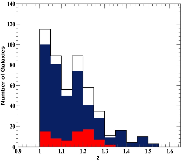
Figure 1. Redshift distribution of the total galaxy sample (black line) used in the coadd to study the outflowing Mg ii gas in bins of Δz = 0.05. Only spectra with coverage of both the Mg ii doublet and the O ii lines are included. This gives us a redshift window of 1.0 ⩽ z ⩽ 1.5. The total sample consists of 486 galaxies with zmedian ∼ 1.1. The redshift distributions of the red galaxies (red histogram) and the blue galaxies (blue histogram) are also shown.
Download figure:
Standard image High-resolution imageEach galaxy is associated with a stellar mass and absolute magnitude as described in the previous section. We divide our sample into blue star-forming and red passive galaxies with their rest frame (U − B) color, which is a weak function of mass. The line dividing red and blue galaxies is given by
where M* is the stellar mass of the galaxy in question and z is the redshift of the galaxy. The color–mass division between blue and red galaxies is shown in Figure 2. The red points are for red galaxies and blue points are for blue galaxies, respectively. After division, we are left with 70 red galaxies and 416 blue galaxies, respectively. The redshift distribution of the red and blue galaxies are shown in Figure 1. The red and blue galaxies essentially have the same N(z). A two-sample KS test cannot rule out the null hypothesis that they are drawn from the same parent distribution at 5% significance.

Figure 2. Target galaxies divided into red and blue galaxies. The red points are for red galaxies and blue points are for blue galaxies, respectively. The galaxies are divided into red and blue galaxies using Equation (1). The horizontal line shows the division between red and blue galaxies.
Download figure:
Standard image High-resolution imageStellar masses (and the SFR) for these galaxies have been estimated by spectral energy distribution (SED) fitting at the known spectroscopic redshifts of the galaxies, using the Hyperzmass code, a modified version of the photo-z code Hyperz (Bolzonella et al. 2010). We refer the reader to Bolzonella et al. (2010) for a detailed technical description of this mass estimation. The absolute magnitudes used in this study were computed as in Zucca et al. (2009). We use the ZEST morphological classification (Scarlata et al. 2007) to estimate the morphologies of the galaxies. This classification is based on the HST/ACS F814W images in the COSMOS field. We compute the flux-averaged star formation rate surface density ( ) of the galaxies by dividing their star formation rates with the area enclosed within their half light radii (R1/2). To study the dependence of galactic outflow on the apparent inclination of the host galaxies, we select only disk dominated galaxies. We identify disk galaxies classified as ZEST type 2, exclude the bulge dominated systems, and divide the sample of galaxies into three bins of inclination angles (i), the face-on galaxies (0° ⩽ i ⩽ 40°), the intermediately inclined galaxies (40° ⩽ i ⩽ 55°), and the edge-on galaxies (55° ⩽ i ⩽ 90°), respectively. This yields a total of 218 disk galaxies. Furthermore, we probe the outflows in the galaxies classified in ZEST to have irregular morphologies, i.e., galaxies with ZEST type 3 which gives a sample of 174 galaxies. The various samples used are shown later in Table 1.
Table 1. Measurements of the Coadded Spectra
| Sample | Wflowa | Woutb | Wallc | 〈Vflow〉d | 〈Vout〉e | 〈Vall〉f | Nog |
|---|---|---|---|---|---|---|---|
| All | 2.52 ± 0.25 | 2.7 ± 0.23 | 4.4 ± 0.22 | −226 ± 32 | −203 ± 63 | −167 ± 51 | 486 |
| Blue log M* ⩾ 10.45 | 3.84 ± 0.42 | 3.72 ± 0.43 | 5.30 ± 0.48 | −244 ± 78 | −213 ± 92 | −196 ± 62 | 126 |
| Blue 10 < log M* < 10.45 | 2.75 ± 0.56 | 2.2 ± 0.51 | 4.80 ± 0.34 | −199 ± 66 | −208 ± 88 | −126 ± 45 | 236 |
| Blue log M* ⩽ 10 | 2.35 ± 0.52 | 2.7 ± 0.53 | 4.8 ± 0.53 | −142 ± 44 | −128 ± 82 | −110 ± 50 | 98 |
| Red | <0.9 | <0.78 | 6.12 ± 0.86 | <−52 | <−45 | 60 ± 80 | 70 |
| log SFR ⩾ 1.5721 | 3.8 ± 0.53 | 3.66 ± 0.56 | 6.02 ± 0.45 | −213 ± 50 | −216 ± 75 | −172 ± 56 | 119 |
| 1.0396 < log SFR < 1.5721 | 2.5 ± 0.42 | 2.9 ± 0.37 | 5.0 ± 0.39 | −153 ± 65 | −140 ± 80 | −120 ± 90 | 237 |
| log SFR ⩽ 1.0396 | 1.8 ± 0.71 | 1.9 ± 0.68 | 4.1 ± 0.74 | −83 ± 58 | −29 ± 85 | −45 ± 50 | 119 |
| 0 ⩽ inc ⩽ 40 | 2.9 ± 0.65 | 2.88 ± 0.73 | 4.38 ± 0.47 | −223 ± 70 | −178 ± 67 | −161 ± 37 | 77 |
| 40 < inc ⩽ 55 | 2. ± 0.64 | 1.95 ± 0.52 | 4.92 ± 0.42 | −83 ± 80 | −59 ± 106 | −50 ± 40 | 87 |
| 55 < inc ⩽ 90 | <0.9 | <0.83 | 4.77 ± 0.50 | < − 23 | < − 12 | 107 ± 146 | 54 |
| Irregulars | 2.95 ± 0.35 | 2.77 ± 0.32 | 5.15 ± 0.35 | −213 ± 79 | −193 ± 62 | −140 ± 35 | 174 |
| log ΣSFR ⩽ −1.04 | <0.79 | <0.83 | 4.72 ± 0.73 | ⋅⋅⋅ | ⋅⋅⋅ | 118 ± 57 | 103 |
| −1.04 < log ΣSFR < −0.25 | 3.0 ± 0.79 | 2.9 ± 0.46 | 4.83 ± 0.41 | -156 ± 101 | −183 ± 102 | −150 ± 60 | 207 |
| log ΣSFR ⩾ −0.25 | 3.6 ± 0.56 | 3.83 ± 0.51 | 5.65 ± 0.47 | −190 ± 51 | −187 ± 92 | −172 ± 55 | 103 |
Notes. aOutflow equivalent width from the decomposition method, in Å. bOutflow equivalent width from boxcar method, in Å. cTotal equivalent width, in Å. dMean outflow velocity from decomposition method, in km s−1. eMean outflow velocity from boxcar method, in km s−1. fMean absorption velocity, in km s−1. gNumber of galaxies.
Download table as: ASCIITypeset image
3. COADDING THE SPECTRA
The spectra of all the galaxies in a particular subsample, are coadded as follows: the systemic redshift of each individual galaxy is redetermined in a uniform way using the [O ii] emission line. Since the spectral resolution of zCOSMOS spectra (R ∼ 600) is not good enough to resolve the [O ii] 3726 Å, 3729 Å doublet, we estimate the systemic redshift of each individual galaxy with detected [O ii] emission at the mean wavelength of the [O ii] doublet weighted by their line ratios (j3729/j3726 = 1.5). This gives a line ratio weighted mean wavelength of the [O ii] line as 3727.7 Å. This line ratio implies that we are assuming a low electron density (ne ≈ 10 cm−3). The bracketing case of assuming a high electron density (ne ≈ 104 cm−3) will put the [O ii] line ratio at ∼0.35 (Osterbrock 1989). This, in turn, implies an offset in the systemic redshift of ≈70–80 km/second, which is comparable to the measured outflow velocity uncertainties. Each spectrum is shifted to its rest frame using the new [O ii] based systemic redshifts. The rest frame spectra are then resampled on a linear wavelength grid with Δλ = 0.6 Å, placing all spectra on a common wavelength scale. Each spectrum is then smoothed with a running median box-car filter with a 39 Å smoothing window and a fifth order polynomial is fitted to determine the continuum level, but excluding the ∼40 Å region around the Mg ii 2796, 2803 doublet and the [O ii] 3727 lines. Each resampled galaxy spectrum is continuum normalized by dividing the galaxy spectrum by this smooth continuum fit described above. Throughout the paper, we use the air wavelengths for all species.
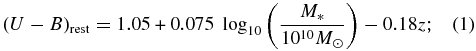
To create the final coadd, a given subset of redshifted, resampled, continuum normalized spectra are coadded by taking the median flux in each wavelength bin. Figure 3 shows the coadded spectrum of a subsample of ∼200 high z (1.15 ⩽ z ⩽ 1.5) galaxies used in this study, these being chosen here because they also show the Fe ii 2600, 2587 lines. The coadded spectrum is dominated by strong [O ii] 3727 emission. There are prominent Balmer absorption lines and the [Ne iii] 3869 emission line is visible. The Ca ii H (3969 Å) and Ca ii K (3934 Å) lines are also visible. The spectrum blueward of the [O ii] 3727 line is relatively featureless except for strong absorption from Mg i at 2852 Å and the Mg ii doublet at 2796, 2803 Å. At the bluest end of the spectrum, the Fe ii 2626 Å emission line is visible and the Fe ii λλ2586 Å, 2600 Å doublets are also seen. In Figure 4, we extract the regions of the coadded spectrum around the Mg ii 2796 Å, 2803 Å doublet and the Mg i 2852 Å line, and plot them on rest frame velocity scales estimated from the [O ii] emission line. The vertical dashed lines give the systemic rest frame zero velocity of each individual line. The first visible signature of outflow can be seen here in the sense that, both the Mg ii and Mg i lines are asymmetric and blueshifted by a few hundred km s−1 with respect to the systemic velocity defined by the rest frame redshift of the [O ii] line.
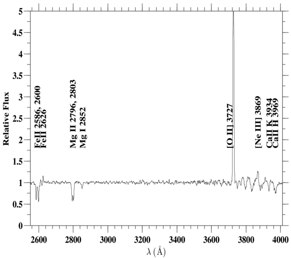
Figure 3. Coadded spectrum of a sample of 207 1.15 ⩽ z ⩽ 1.5 zCOSMOS galaxies in their rest frame. All the galaxies are continuum normalized to one. The spectrum is smoothed with a 5 Å boxcar.
Download figure:
Standard image High-resolution image
Figure 4. Mg ii 2796, 2803, and Mg i 2852 lines in the coadded spectrum of the full sample of 486 zCOSMOS galaxies. The Mg ii 2803 and Mg i 2852 lines are shifted to their systemic zero velocities. The systemic zero velocities are defined by the galaxy redshifts derived from their [O ii] emission lines. The Mg ii and the Mg i lines show blueshifted and asymmetric absorption profiles. The vertical dashed lines show the systemic zero velocities for each transition respectively.
Download figure:
Standard image High-resolution image4. MEASURING THE OUTFLOWING COMPONENT TRACED BY Mg ii ABSORPTION
In this section, we describe two methods that are used in the rest of the paper to assess the absorption strength of the blueshifted outflowing gas and the mean velocities. In both methods, we estimate the absorption strength of the systemic component by analyzing the red side of the Mg ii 2803 Å line. We then estimate the total absorption strength due to the systemic component in the Mg ii doublet and "recover" the absorption strength of the outflowing gas by comparing the systemic component with the observed absorption profile. This "recovered" outflowing component is corrected for low spectra resolution effects to yield the final outflow absorption strength. The two methods are described as follows.
4.1. Decomposition Method
This method is based on the decomposition method described in Weiner et al. (2009). We first remove the systemic ISM absorption component from the coadded spectra and then proceed to identify the strength of the outflowing gas in the coadd. The outflowing gas lying between the observer and the light source (the galaxy) will absorb photons at blueshifted negative velocities with respect to the systemic redshift of the galaxy. This outflowing gas could have some velocity dispersion (generally much lower than the thermal broadening of individual clouds) and even complex kinematic structures. However, due to the low resolution of the zCOSMOS spectra, such kinematic complexities can be neglected for the present purposes. The model describing the final observed absorption line is


where Fobs(λ) is the observed flux density from the coadded spectra, C(λ) is the fit to the local continuum of the coadded spectra, Fem(λ) describes any emission above the continuum level and for simplicity is set to unity. [1 − Asym(λ)] describes the systemic absorption component and [1 − Aflow(λ)] describes the absorption profile due to outflowing (blueshifted) gas. The symmetric absorption component is taken to be the sum of two Gaussians centered at the rest frame wavelength of each component of the Mg ii λλ2796 Å, 2803 Å doublet.
The decomposition of the symmetric and the outflowing component can be a complex problem due to the doublet structure of the absorption profile. We, therefore, infer the symmetric component by fitting a Gaussian on the red side of the 2803 Å line (within 0 km s−1 ⩽ v ⩽ 1500 km s−1). Since the Mg ii doublet is partially blended in our coadd, assuming symmetry, we impose the Gaussian fitted to the 2803 line onto the 2796 line as well. We keep the depth of these two Gaussians the same (A2796 = A2803), as the individual Mg ii lines are likely to be saturated. If these absorption lines are not completely saturated, then it may happen that the 2796 Å line is slightly deeper than the 2803 Å line. In that case, we will underestimate the systemic component in that line.
The results of this approach are illustrated in Figure 5. The black line is the observed spectrum, the red dashed double Gaussian is the symmetric component [1 − Asym(λ)], and the blue line is the detected outflowing component [1 − Aflow(λ)].
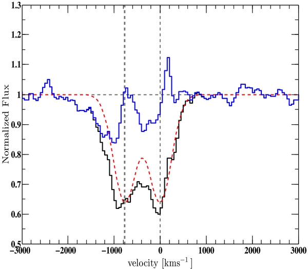
Figure 5. Mg ii absorption doublet in the coadded spectrum of the full sample of 486 galaxies (solid black line). The vertical dashed lines show the systemic zero velocities for each transition, respectively. The dashed red line shows the Gaussian systemic absorption model profile fit given by Equation (3). The solid blue line shows the outflowing absorption profile inferred from Equation (2).
Download figure:
Standard image High-resolution imageThe total outflow equivalent width is the equivalent width of the outflowing component measured between −1500 km s−1 ⩽ v ⩽ 0 km s−1 with respect to the 2803 Å line and, therefore, include both the components of the doublet. It should, therefore, be noted that the quoted outflowing equivalent width throughout the paper is the total equivalent width of the outflowing components from both the 2796 Å and the 2803 Å lines. The mean outflow velocity (〈vflow〉) is the mean velocity of the outflowing gas blueward of the zero velocity of the 2803 Å line up to a velocity adaptively chosen to be the point at which the absorption is absent or minimized and never greater than −768 km s−1. We also calculate the mean outflow velocity with respect to the 2796 Å line, and the measured outflow velocities from both the Mg ii 2796 and 2803 lines are consistent within the uncertainties. Throughout the paper, we quote the outflow velocity with respect to the 2803 Å line.
The errors on the equivalent width as well as the outflow velocities are estimated using a bootstrap approach. For each set of galaxy spectra to be coadded, a thousand coadded spectra are generated by randomly selecting spectra from that sample. For each of these coadds, the outflow equivalent width and the mean outflow velocities are estimated. The width of the distribution of the measured equivalent widths and the outflow velocities in these thousand coadds are taken as representative of the error in the original measurements and should also account for sample variance, continuum uncertainties, and the error in fitting the decomposition model.
This method assumes that the outflowing profile described in Equation (2) is only due to absorption from outflowing gas. Any redshifted emission in the 2803 Å line will change the amplitude and the width of the Gaussian fitted to the symmetric component. Emission to the red side of the 2796 Å line will effectively cause us to underestimate the equivalent width of the outflowing gas. It is very hard to account for the emission filling because the strength of Mg ii emission lines will depend on the galaxy mass as well as the dust content of the galaxy (see Kornei et al. 2013 and Martin et al. 2012 for a more detailed description of Mg ii emission lines). We are also assuming that there is a negligible amount of gas falling into the galaxy. Infalling gas can also contribute to the red wing of the 2803 Å absorption. However, recent observations of individual galaxy spectra have shown that the covering fraction of infalling gas is quite low, approximately ∼6 % (Rubin et al. 2012; Martin et al. 2012). Moreover, the equivalent widths of the inflowing component is always lower than that of the outflowing component, and hence it can only be observed when there is little or no outflow. Because of these considerations, we shall neglect the inflowing component in the reminder of this study.
It should be noted that this method works optimally for high S/N spectra, as for such cases the symmetric component can be modeled accurately and hence gives a better estimate of the outflowing gas.
4.2. Boxcar Method
To estimate the equivalent width of the outflowing gas, we also use a second method similar to the method used by Rubin et al. (2010). This method is more accurate for low S/N coadds as compared to the decomposition method. We make an assumption that the Mg ii doublet is saturated near the systemic velocities, in our spectra, such that the systemic components of 2796 Å and 2803 Å lines have the same depths at v = 0 km s−1. This is a reasonable assumption because the Mg ii absorption line becomes saturated at column densities ∼1014 cm−2, which correspond to relatively low hydrogen column densities >1019 cm−2 at solar abundance (Rubin et al. 2010). The contribution from the ISM and the stellar atmosphere, which likely makes the dominant contribution to the systemic absorption, typically have column densities exceeding these values.
We measure the outflow equivalent width as follows

where
and Fobs(λ) is the observed coadded spectra and C(λ) is the local continuum around the absorption feature. W2803 Å, red is the amount of absorption due to gas that is not outflowing, this is subtracted from W2796 Å, blue to avoid overestimating the outflow absorption strength due to inclusion of the systemic component of absorption. This difference is multiplied by two to give the total equivalent width of the outflowing component in the doublet Wout. This method is more reliable for low S/N spectra because, as opposed to the decomposition method, this method does not directly rely on modeling the systemic component.
To estimate the mean outflow velocity in this second method, we consider the mean absorption weighted outflow velocity
since we can assume that the mean velocity of the systemic component (〈vsym〉) is zero. Wall is the total equivalent width of the Mg ii 2796, 2803 doublet and 〈vall〉 is the mean absorption weighted velocity of the observed absorption line Fobs(λ) with respect to its systemic velocity.
The errors of measurement in this method are estimated similar to the decomposition method. Out of the sample of galaxies under study, randomly selected spectra are coadded one thousand times. For each coadd equivalent widths and velocities are measured as described above. The width of the distribution of the measured equivalent widths and the velocities in these thousand coadds are taken as representative of the error in the original measurements.
4.3. Correction for Spectral Resolution
Both methods described above assume that there is no redshifted absorption from the outflowing gas. However, we are dealing with finite spectral resolution, which effectively puts some of the absorption from the outflowing gas into the redshifted absorption. This implies that we will overestimate the systemic component and as a result the outflow equivalent widths will be underestimated as the spectral resolution is degraded.
To estimate the typical magnitude of this effect, we set up a simple empirical model, similar to the model described by Equations (2) and (3). We set up a systemic absorption component described as [1 − Asym(λ)] centered on the Mg ii 2796, 2803 absorption doublet. The depths of the two Gaussians are ∼40% of the continuum (we assume that the systemic component is saturated and hence the line ratio is 1:1) and σsym = 100 km s−1 is chosen. The outflowing component [1 − Aflow(λ)] can be of any arbitrary shape, but we assume that it can also be described by two Gaussian profiles that are blueshifted from the systemic velocity by an arbitrary velocity offset Δv, which is varied. The Gaussians describing the outflowing components are truncated at zero velocity. The depth of the outflowing absorption profile is also varied and the width of the outflowing component varied to be Δv/2 ⩽ σout ⩽ Δv. We again assume that there is no emission and get an ideal absorption profile  . To account for finite spectral resolution
  is convolved with a Gaussian window function W to give the observed flux F(λ) as follows
Here, W is a Gaussian with an FWHM that is changed to mimic the effect of varying resolution. The equivalent width of the outflow component is then estimated from F(λ) using both the decomposition and the boxcar method. Figure 6 shows the observed equivalent width of the outflow component for a set of models with a fixed systemic component and varying outflow component chosen to span an outflow velocity range of −326 km s−1 ⩽ 〈vout〉 ⩽ −195 km s−1. For a model with an intrinsic outflow equivalent width of ∼2.7 Å, the observed outflow equivalent width is ∼1.55 Å for an instrument with an FWHM of 500 km s−1. This correction needs to be applied to the measurements done with both the decomposition and the boxcar method to estimate the true outflow equivalent width corrected for resolution effects.

Figure 6. Variation in estimating the outflow equivalent width as the resolution of the spectra is degraded. Five models with different outflow velocities (〈Vout〉) are considered. The intrinsic outflowing equivalent width (Wflow at FWHM=0) is underestimated as the spectra are convolved with the instrumental FWHM.
Download figure:
Standard image High-resolution imageThe Mg ii absorption doublet from the coadd of all the 486 galaxies was shown in Figure 5. Before correcting for resolution, the outflow equivalent width measured from the decomposition method is Wflow = 1.42 Å and the outflow equivalent width measured from the boxcar method is Wout = 1.6 Å. Since the resolution of zCOSMOS spectra corresponds to an FWHM of ∼500 km s−1, the resolution corrected outflow equivalent widths are Wflow = 2.52 ± 0.25 Å and Wout = 2.7 ± 0.23 Å, respectively. The outflow velocities inferred by both the methods are 〈vflow〉 = − 293 ± 32 km s−1 and 〈vout〉 = − 270 ± 63 km s−1, respectively. 〈vout〉 is estimated using Equation (7). It should be noted that Wall and 〈vall〉 are not affected by the degradation in resolution and hence are robustly estimated from the observed absorption feature without any corrections. As a result, the use of Equation (7) to deduce 〈vout〉 only requires the correction of Wout. These outflow velocities are not taking into account, emission filling because of redshifted backscattered Mg ii emission. We account for this effect by applying an average correction of 67 km s−1 to all the outflow velocity estimates. This correction gives emission corrected 〈vflow〉 = − 226 ± 32 km s−1 and 〈vout〉 = − 203 ± 63 km s−1, respectively. The average correction for emission filling is obtained by comparing the Mg ii and Fe ii outflow velocities at higher redshifts as described below. Throughout the paper, all of the outflow velocities quoted were found after correcting for an average emission filling.
4.4. Fe ii 2586, 2600 Absorption
In this section, we measure outflow velocities using the Fe ii 2586, 2600 lines and check that these velocities are indeed consistent with that measured with the blueshifted Mg ii doublet. Fe ii lines have the added value that they will suffer less from redshifted emission filling, allowing a robust characterization of the systemic component (Prochaska et al. 2011). However, they are too blue to be observed in our spectra at all redshifts. The Fe ii 2586, 2600 doublet can only be analyzed with our sample at z > 1.15. We select a subsample of 207 galaxies with z > 1.15, which are coadded and used to analyze the Fe ii doublet. We continuum normalize and coadd the spectra as before. Figure 7 shows the coadded Fe ii 2586, 2600 lines as well as the corresponding Mg ii 2796, 2803 doublet, respectively. The Mg ii doublet is offset vertically for presentation. We model the systemic components of the Fe ii 2586, 2600 lines by fitting a single Gaussian on the red side of both lines independently (Figure 7, red lines). The blue lines show the estimated outflowing component for both the transitions. The Fe ii 2586, 2600 outflow equivalent widths are almost the same for both lines (W2586 = 0.85 ± 0.30 Å, W2600 = 0.98 ± 0.29 Å), indicating that the outflowing gas is optically thick in the coadd. We compute for the same coadded spectra the Mg ii outflow equivalent width, Wflow = 2.1 ± 0.36 Å. We obtain the mean outflow velocity for each species as before and find for the Fe ii 2586 line 〈Vflow〉(2586) = −223 ± 62 km s−1 and for the Fe ii 2600 line 〈Vflow〉(2600) = −259 ± 75 km s−1. For the Mg ii transition, we estimate the mean outflow velocity 〈Vflow〉(2803) = −290 ± 47 km s−1 and 〈Vflow〉(2796) = −285 ± 53 km s−1. Hence, the measured mean outflow velocities are consistent within the uncertainties for both Mg ii and Fe ii doublets. However, the inferred mean Fe ii outflow velocities are slightly lower than the mean outflow velocities inferred from the Mg ii absorption. This is owing to the fact that emission filling in the Mg ii doublet will systematically create bias, leading us to underestimate the systemic absorption components. The difference between 〈Vflow〉(2803) and 〈Vflow〉(2586) is 67 km s−1. However, the general trends seen regarding dependence of galactic outflows with galaxy properties will remain the same for both the absorption species. We compensate the effect of emission filling by applying an average correction of 67 km s−1 to all Mg ii traced outflow velocity estimates. Throughout this study, all of the outflow velocities are offset by 67 km s−1 to compensate the effect of backscattered redshifted emission filling.

Figure 7. Estimating outflow velocities for Fe ii 2586, Fe ii 2600, Mg ii 2796, and Mg ii 2803 lines from the coadded spectrum of the z > 1.15 subsample. The Mg ii doublet has been offset vertically for presentation. The coadded spectra for both Mg ii and Fe ii (black lines) are shown here. The decomposed systemic(red) and outflowing(blue) profiles are also shown. Both the Mg ii doublets and the Fe ii lines exhibit outflow velocities consistent within the uncertainties.
Download figure:
Standard image High-resolution image5. RESULTS
In the following section, we discuss the variation of equivalent widths and velocities of outflowing gas traced by the Mg ii absorption with the different properties of the host galaxies, examining the dependence on rest frame color, mass, star formation rate, star formation rate surface density (ΣSFR), and, for the disk galaxies, the apparent inclination. The measurements are tabulated in Table 1.
5.1. Dependence on Color and Mass
We first investigate the variation of the outflow equivalent width and outflow velocity with the rest frame color and stellar mass of the host galaxies. The galaxy sample is divided into red and blue galaxies as described before. To study the mass dependence, we divide the blue galaxies into three stellar mass bins. The low-mass blue galaxy sample consists of galaxies with M* ⩽ 1010M☉, the intermediate-mass blue galaxy sample consists of galaxies with stellar masses 1010M☉ < M* ⩽ 1010.45M☉ and the high mass blue galaxy sample is defined as galaxies with M* > 1010.45M☉
The high mass blue galaxy sample has a mean stellar mass 〈M*〉 = 1010.71 ± .22M☉, which is reasonably close to the mean mass of the red galaxy sample 〈M*〉 = 1011 ± .24M☉ to compare the dependence of outflowing properties with color. Figure 8 shows the variation of outflow equivalent width as a function of rest frame color and stellar mass. It can be seen that both the decomposition method (filled circles), and the boxcar method (open diamonds) give similar outflow equivalent widths within the uncertainties. Among the blue galaxies, the high-mass blue galaxies exhibit higher outflow equivalent widths as compared to the low mass blue galaxy samples. At similar stellar mass ranges, the blue galaxies exhibit significantly higher outflow equivalent widths as compared to the red galaxies. In the sample of red galaxies, very little outflow absorption is observed. This color and mass dependence in the equivalent width of the outflowing component hints at a dependence of the outflowing gas on the star formation rate of the host galaxy. This trend is also similar to the trend observed in Bordoloi et al. (2011) for impact parameters within 50 kpc of 0.5 ⩽ z ⩽ 0.9 galaxies, seen in the spectra of background galaxies.

Figure 8. Variation of the outflow equivalent width as a function of color and mass of the host galaxies. The blue galaxies (blue points) exhibit a rise in equivalent width with stellar mass. At similar stellar mass ranges, the blue galaxies have significantly higher outflow equivalent widths as compared to red galaxies (red point). The measurements done with the decomposition method are represented by (red and blue) filled circles and the measurements done with the boxcar method are represented by (red and blue) open diamonds. The gray open circles are measurements from Weiner et al. (2009) and the gray open diamonds are measurements taken from Rubin et al. (2010). The error bars on the x axis are standard deviations of the masses in each bin. The blue diamonds are offset in mass by 0.1 dex for clarity.
Download figure:
Standard image High-resolution imageThe gray points are data points taken from the literature, the gray open circles are taken from Weiner et al. (2009) and the gray open diamonds are taken from Rubin et al. (2010). The study done in Weiner et al. (2009) used 1406 spectra of blue star forming galaxies at z ∼ 1.4 from the DEEP2 galaxy survey. They estimated the outflow equivalent width of the 2796 Å line only and we have multiplied that value by two to compare with our estimates of the total outflow equivalent width of the doublet. The study done in Rubin et al. (2010) used a sample of 468 galaxies in the TKRS survey in the GOODS-N field at 0.7 ⩽ z ⩽ 1.5 with a median redshift of 0.9. Both of these studies have a higher spectral resolution than the zCOSMOS bright survey. Although these studies were done in different redshift ranges, their general trends are consistent with our finding of a general increase of outflow equivalent width with stellar mass. We perform a Pearson linear rank correlation test, which rules out the null hypothesis that there is no correlation between stellar mass and outflow equivalent width among blue galaxies at a 95% confidence level. Our own analysis highlights the importance of incorporating color in interpreting the trends with mass and/or luminosity.
Figure 9 shows the outflow velocity estimates done with both the decomposition and the boxcar method as a function of stellar mass. For the red galaxies, only an upper limit for outflow velocity is measured. The gray points are again taken from Weiner et al. (2009). We find that, within the error bars, there is no significant trend in outflow velocity as a function of stellar mass, although the low mass blue sample gives a lower estimate of outflow velocity in the boxcar method as compared to the decomposition method. In general, we find a typical range of outflow velocity ranging approximately from −150 to −200 km s−1 among these galaxies.

Figure 9. Variation of outflow velocity as a function of mass of the host galaxies. The measurements done with the decomposition method are represented by filled circles and the measurements done with the boxcar method are represented by open diamonds. The gray open circles are measurements from Weiner et al. (2009). The error bars on the x axis are standard deviations of the masses in each bin. The blue diamonds are offset in mass by 0.1 dex for clarity.
Download figure:
Standard image High-resolution image5.2. Dependence on SFR
In this section, we investigate the correlation between the star formation rates and the outflow properties of the galaxies. The galaxy sample is subdivided at the 25th and 75th percentile values of star formation rates. The lowest star forming sample consists of galaxies with log10(SFR/M☉ yr−1) ⩽ 1.0396. The intermediate star forming sample consists of galaxies with 1.0396 < log10(SFR/M☉ yr−1) ⩽ 1.572. The highest star forming sample is made out of galaxies with log10(SFR/M☉ yr−1) > 1.572.
Figure 10 shows the variation of outflow equivalent width as a function of the star formation rate of the galaxies. There is a general trend of steady increase in outflow equivalent width with increasing star formation rates. This trend is seen in both the decomposition method estimates and the boxcar estimates. These trends are consistent with the trends found in the literature (gray points) though the other studies were done at different redshift ranges.

Figure 10. Variation of outflow equivalent width as a function of the star formation rate of the host galaxies. The measurements done with the decomposition method are filled circles and the measurements done with the boxcar method are open diamonds. The gray open circles are measurements from Weiner et al. (2009) and the gray open diamonds are measurements from Rubin et al. (2010). The blue diamonds are offset in SFR for clarity.
Download figure:
Standard image High-resolution imageFigure 11 shows the variation of outflow velocity with varying star formation rates. We find that the mean velocity of the total Mg ii absorption (〈vall〉) increases with the increase of SFR (see Table 1), the inferred outflow velocities also show a very weak trend of increasing with SFR. Owing to large uncertainties in our measurements, both estimates are broadly consistent with the observations of Weiner et al. (2009; gray circles), who found a weak correlation between increasing outflow velocity with increasing star formation rates. The outflow velocity estimates in Weiner et al. (2009) are not corrected for emission filling, which accounts for the small offset with our outflow velocity estimates. Combining our measurements with that from Weiner et al. (2009), we perform a Pearson linear rank correlation test and find a 2.7σ correlation between log SFR and equivalent width/outflow velocity.

Figure 11. Variation of outflow velocity width as a function of star formation rate of the host galaxies. The measurements done with the decomposition method are filled circles and the measurements done with the boxcar method are open diamonds. The gray open circles are measurements from Weiner et al. (2009) and the gray open diamonds are measurements from Rubin et al. (2010). The blue circles are offset in SFR for clarity.
Download figure:
Standard image High-resolution image5.3. Dependence on ΣSFR
In this section, we test for dependence of outflow strength on the SFR surface density (ΣSFR). We estimate a flux-averaged SFR surface density ( ), for each object assuming that star formation is distributed like the (observed frame) i-band light (i.e., half the star forming regions of the host galaxies are within their half light radius (R1/2)). The left panel of Figure 12 shows the distribution of log SFR and
  for the sample used in this section. The red and cyan lines indicate the 25th and the 75th percentile values of log ΣSFR (−1.04, −0.25), which are used to subdivide our sample.

Figure 12. Left panel:  vs. log SFR for the target galaxies. Lines show subdivision in log ΣSFR. Right panel: variation of outflow equivalent width as a function of ΣSFR. The measurements done with the decomposition method are represented by filled circles and the measurements done with the boxcar method are represented by open diamonds. The blue diamonds are offset in SFR for clarity. The vertical dashed line shows the canonical threshold in star formation surface density for driving winds (ΣSFR = 0.1 M☉ yr−1 kpc−2). Galaxies above this threshold have strong outflow equivalent widths, but, below this threshold, we detect only an upper limit for outflowing equivalent width.
Download figure:
Standard image High-resolution imageIn Figure 12, the right panel shows the outflow equivalent width versus log ΣSFR. The filled circles are measurements done with the decomposition method and the open diamonds are estimated with the boxcar method. The subsample with the lowest log ΣSFR exhibits very little outflow equivalent width and as we probe the higher log ΣSFR subsamples the measured outflow equivalent width increases.
It is interesting to discuss these results in the context of the canonical star formation rate surface density "threshold" (ΣSFR = 0.1 M☉ yr−1 kpc−2). It has been suggested that it is the minimum ΣSFR required for driving outflows in local starbursts (Heckman 2002). By chance, this threshold corresponds to the ΣSFR between the first and the second bin in this study, and it is noticeable that the lowest bin has only an upper limit for outflowing equivalent width. The Pearson linear rank correlation test shows a 2.9σ correlation between log ΣSFR and outflow equivalent width.
At higher redshifts, Rubin et al. (2010) and Steidel et al. (2010) have reported weaker correlations of outflow absorption strength with ΣSFR. Recently, Kornei et al. (2012) reported a 3.1σ correlation of outflow velocity with ΣSFR at these redshifts. At z ∼ 2, Newman et al. (2012) reported a correlation between outflow strength (quantified via the broad flux fraction of the Hα line) and ΣSFR of star forming galaxies. They reported a ΣSFR threshold of 1 M☉ yr−1 kpc−2, above which M* > 1010M☉ galaxies might have stronger outflows as compared to the low mass galaxies.
5.4. Dependence with Apparent Inclination Angle of Disk Galaxies
In this section, we present the variation of Mg ii outflow kinematics with the apparent inclination of the associated disk galaxies. We select the galaxies to be disk-dominated, as described before. We divide the disk galaxies into three bins in inclination angles, with 0° ⩽ i ⩽ 40°, 40° < i ⩽ 55°, and 55° < i < 90°. The definition of the inclination angle is such that i = 90° represents an edge-on system and i = 0° represents a face-on system. Some examples of the typical galaxies selected are shown in Figure 13. We also investigate the distribution of mass, SFR, and ΣSFR in each inclination bin and find that they are consistent with having the same parent distribution according to a two-sample KS test at a 10% significance level. The cumulative distributions of the stellar mass, SFR, and ΣSFR of the galaxies in each inclination bin are shown in Figure 14.

Figure 13. HST/ACS images of the galaxies with different inclination angles. The inclination angles are shown in the top left corner of the stamps. The extreme right galaxy is classified as having an irregular morphology with ZEST type 3. The disk galaxies are chosen not to include bulge dominated systems.
Download figure:
Standard image High-resolution image
Figure 14. Cumulative distribution of mass, SFR, and ΣSFR of the galaxies with different inclinations and irregular morphologies. The two-sample KS test performed on the different distributions show that the null hypothesis that the disk galaxies are drawn from the same parent distributions cannot be ruled out at a 10% significance level. The mass, SFR, and ΣSFR distribution of irregular galaxies, when compared with that of the disk galaxies, shows that the null hypothesis that they are drawn from the same parent mass distribution can be ruled out at a 5% significance level.
Download figure:
Standard image High-resolution imageFigure 15 shows the variation of outflow equivalent width (left panel) with inclination and outflow velocity (right panel) with inclination. The error bars in inclination angles are the standard deviation of the inclination angles within that bin. The face-on systems show the strongest outflow absorption equivalent width and this decreases with increasing inclination. The edge-on systems show the weakest outflow equivalent width and only a 1σ upper limit was measured in both the decomposition (filled circles) and the boxcar (open diamonds) methods. The face-on systems also exhibit the highest outflow velocities and the observed outflow velocities decrease as we probe galaxies with higher inclinations. The Pearson linear rank correlation test shows a 3σ correlation between galaxy inclination and outflow equivalent width/outflow velocities.
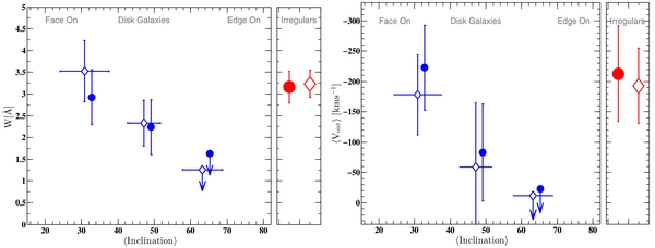
Figure 15. Variation of outflow equivalent width (left panel) and outflow velocity (right panel) as a function of the apparent inclination of the disk galaxies. Open diamonds are boxcar measurements and the filled circles are decomposition measurements. Error bars on the x-axis are standard deviations in the inclination bin. The face-on galaxies clearly exhibit higher outflow equivalent widths and outflow velocities as compared to the edge-on galaxies. The red points are measurements for galaxies with irregular morphologies. The irregular galaxies exhibit outflows as strong as the face-on galaxies. The blue diamonds are offset in inclination angle for clarity.
Download figure:
Standard image High-resolution imageThe galaxies with irregular morphologies, classified as ZEST type 3 have similar outflow equivalent widths as the face-on disk galaxies and similar outflow velocities (∼ − 200 km s−1, red points Figure 15). Since no inclination can be assigned to the galaxies with irregular morphologies, their outflow estimates are essentially averaged over all possible orientations. However, it should be noted that the mass distribution of these galaxies is not the same as that of the disk galaxies. A two-sample KS test performed on the distribution of mass, SFR, and ΣSFR of the irregular and disk galaxies rules out the null hypothesis that they are drawn from the same parent distribution at a 5% significance level. To the first order, they are shifted to lower mass by about 0.15 dex in mass and 0.3 dex is SFR.
The trend of variation of outflow velocity with galaxy inclination is similar to the trends observed for low-redshift samples. Chen et al. (2010) studied a sample of ∼150,000 SDSS galaxies and created stacks of galaxy spectra as a function of apparent disk inclination and studied the outflow properties of the Na D absorption doublet. They found a strong increase in outflow velocity as the galaxies became more and more face-on, which is consistent with the picture of galactic winds escaping along the disk rotation axis. Furthermore, Heckman et al. (2000) observed Na D absorption in 18 local starbursts and found that a higher fraction of the face-on galaxies exhibit outflows as compared to the edge-on systems. These low-redshift studies were feasible because of relatively bright targets and high resolution spectroscopy.
Recently, Weiner et al. (2009) examined 118 galaxies at z ∼ 1.4 with HST I-band imaging and did not find a correlation between apparent inclination and wind strength or outflow velocity. They inferred that this might be due to uncertainties in estimating axis ratios of irregular galaxies imaged in the rest-frame U band. Kornei et al. (2012), using a sample of 72 z ∼ 1 galaxies, divided their sample at i = 45° and found that the coadded spectra of the face-on systems exhibit higher outflow velocity as compared to the more edge-on systems.
Our results for inclination dependence of outflowing gas in the "down the barrel" spectra of disk galaxies are entirely consistent with the azimuthal dependence (around edge-on galaxies) of the distributed strong Mg ii absorbers, seen against the spectra of background galaxies in Bordoloi et al. (2011).
The new results tie directly to the picture that the azimuthal asymmetry of strong Mg ii absorption line systems around galaxies, observed in the spectra of background galaxies or quasars, are primarily due to cool Mg ii gas entrained in star-formation-driven bipolar winds, especially at low impact parameters (Bordoloi et al. 2011, 2014).
6. MASS OUTFLOW RATE
The amount of gas ejected in galactic outflows is of great interest because it allows us to understand its importance in galaxy evolution (see, e.g., Lilly et al. 2013). This is, however, not trivial to estimate. The Mg ii lines observed are optically thick and would be approaching the flat part of the curve of growth. Hence, their column densities cannot be inferred from their equivalent widths. We will, therefore, estimate their apparent optical depths and hence their apparent column densities, which will give a conservative lower limit of the column density of Mg ii gas. The apparent optical depth of the line is given as
The apparent column density per velocity element, Na(v) is given as

where log fλ0 = 2.933 for the Mg ii 2803 line (Morton 1991). We compute τa(v), between 0 and −768 km s−1 of the Mg ii 2803 line.
The integrated apparent column density Na, which we take as the lower limit of the true column density of the outflowing gas, is obtained as
We apply this procedure to estimate the column density of outflowing gas for the full sample of 486 galaxies and find log N(Mg ii) > 13.63, and, for the sample with the highest ΣSFR, we find log N(Mg ii) > 13.87.
To estimate a conservative lower limit to NH in the outflow, we assume no ionization correction (N(Mg) = N(Mg ii)), and take the minimum column density for Mg ii with no correction for saturation. We assume a solar abundance of Mg, log Mg/H = −4.42 and assume a factor of −1.3 dex of Mg depletion onto dust (Jenkins 2009). This gives a column density of log NH ⩾ 19.34 for the whole sample and log NH ⩾ 19.6 for the highest ΣSFR bin. We stress that this estimate of column density of outflowing gas is a lower limit because we are neglecting ionization correction and underestimating any effects of saturation. Moreover, any redshifted emission from the Mg ii 2796 line will also reduce any blueshifted absorption from the Mg ii 2803 line, further reducing the computed column densities here. On the other hand, dust depletion might be less for high velocity outflows.
The mass outflow rate for a wind with opening angle Ωw is given as

where CΩ is the angular covering fraction and Cf is the clumpiness covering fraction, μmp is the mean atomic weight, R is the minimum radius of the outflowing gas, and v is the mean velocity of the outflowing gas. Since the composite spectra of galaxies are viewed from all angles and the composites integrate over all small-scale line-of-sight clumpiness as well as the partially and fully covered lines. Hence, we set CΩCf = 1 and Ωw = 4π (thin shell approximation). Setting μ = 1.4, we rewrite the mass outflow rate as (see Weiner et al. 2009)
We do not have any constraints on the spatial extent of the outflowing gas. However, it must be at least of the order of the size of the galaxies, since the covering factor is large. Hence, we use the median half light radius of our galaxy sample as the minimum radial extent of the winds (R ∼ 4.1 kpc).
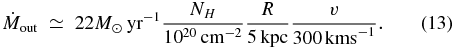
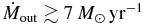
Putting in all the values, we find that, for the whole sample, the mass outflow rate is  and for the highest ΣSFR sample it is
  . These values are consistent with previous works (Weiner et al. 2009; Rubin et al. 2010; Martin 2005; Newman et al. 2012) and we find that
  is of the order of the star formation rate of the sample. Assuming that mass outflow rates are directly proportional to the star formation rate of the galaxies (
 ), we can put lower limits on the mass loading factor η. We find that, for the whole sample, the average mass loading factor is η ≳ 0.24. Again these values are conservative lower limits and better measurements on R and NH are needed to constrain the mass outflow rates further.
7. CONCLUSIONS
In this work, we have analyzed the coadded spectra of (R ∼ 600) 486 zCOSMOS galaxies at 1 < z < 1.5 to study the properties of galactic outflows using Mg ii absorption lines as tracers. We divided our sample in terms of the rest frame color, mass, and star formation rates of the galaxies and studied the properties of outflow equivalent width and outflow velocity. Finally, we examined how outflow kinematics depend on the apparent inclination of disk galaxies and compared the findings to those of galaxies with irregular morphologies. The main findings of this study are as follows.
- 1.We find that the whole sample of 486 galaxies exhibits blueshifted absorption with a mean outflow velocity of vflow = −226 ± 32 km s−1 and vout = − 203 ± 63 km s−1 measured with the decomposition and the boxcar method, respectively. The total outflow equivalent width for the stacked spectrum is measured to be Wflow = 2.52 ± 0.25 Å and Wout = 2.7 ± 0.23 Å, respectively.
- 2.We find that the blue galaxies are associated with a much stronger outflowing component as compared to the red galaxies in terms of their rest frame equivalent widths. At similar mean stellar masses, the blue galaxies exhibit almost four times higher outflow equivalent width as compared to the red galaxies.
- 3.Among the blue galaxies, the outflow equivalent width also increases with increasing stellar mass. The uncertainties in outflow velocity estimates do not allow us to firmly establish an increase in outflow velocity with stellar mass of the host galaxies. Our findings also emphasize the need to consider the color of the galaxy in examining outflow trends with stellar mass or luminosity (as massive red galaxies show little outflow).
- 4.We find that galaxies with higher star formation rates exhibit higher outflow equivalent widths. There may be a correlation between outflow velocity with star formation rate, but due to large uncertainties in outflow velocity estimates this is of weak statistical significance.
- 5.Galaxies with high ΣSFR exhibit strong outflow equivalent widths as well as mean outflow velocity. We detected no outflow in the sample with ΣSFR ⩽ 0.1 M☉ yr−1 kpc−2 consistent with the canonical ΣSFR threshold found at low redshifts.
- 6.Among the disk galaxies, the galaxies that are seen close to face-on (inclination i ⩽ 40°) are found to have ∼2.5 times higher outflow equivalent widths as compared to the galaxies that are more close to being edge-on (inclination i ⩾ 55°). In terms of outflow velocities, the face-on systems are also found to have higher outflow velocities (∼ − 200 km s−1) as compared to the edge-on systems, where only an upper limit of ⩽ − 23 km s−1 was detected. This dependence on inclination suggests that for the disk galaxies, the galactic outflow is bipolar in nature and is primarily perpendicular to the disk of the galaxy.
- 7.For galaxies with irregular morphology, we find a relatively high outflow equivalent width and outflow velocity comparable to that of the face-on galaxies.
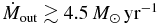
- 8.We also present lower limits on mass outflow rates (
 ), which, for the whole sample, is and, for the highest ΣSFR sample, it is . Assuming , we find that the average mass loading factor η for the whole sample is η ≳ 0.24.


R.B. thanks Jason Tumlinson for stimulating discussions and for carefully reading through the draft and giving insightful comments. This work has been partly supported by the Swiss National Science Foundation and is based on observations undertaken at the European Southern Observatory (ESO) Very Large Telescope (VLT) under Large Program 175.A-0839.
Footnotes
- *
Based on observations undertaken at the European Southern Observatory (ESO) Very Large Telescope (VLT) under Large Program 175.A-0839.