


ABSTRACT
We present new insights into the physical nature of coronal mass ejections (CMEs) and associated shock waves within the framework of the three-dimensional (3D) structure. We have developed a compound model in order to determine the 3D structure of multiple fronts composing a CME, using data sets taken from STEREO, SDO, and SOHO. We applied the method to time series observations of a CME on 2012 March 7. From the analyses, we revealed that a CME could consist of two different fronts: one is represented well with the ellipsoid model, implying that CMEs are bubble-shaped structures, and the other is reproduced well with the graduated cylindrical shell model, indicating that CMEs are flux rope-shaped structures. The bubble-shaped structure is seen as the outermost front of the CME, and the flux rope-shaped structure is seen as the bright frontal loop or three-part morphology. From our results, we conclude that (1) a CME could consist of two distinct structures, a bubble-shaped structure and a flux rope-shaped structure, (2) the bubble-shaped structure is a fast magnetosonic shock wave, while the flux rope-shaped structure is the mass carried outward by the underlying magnetic structure, (3) the driven shock front could be either a piston-shock type or a bow-shock type, (4) the observed EUV wave in the low corona is the footprint of the bubble-shaped wave, and (5) the halo CME is primarily the projection of the bubble-shaped shock wave but not the underlying flux rope.
Export citation and abstract BibTeX RIS
1. INTRODUCTION
Coronal mass ejections (CMEs) are the most spectacular eruptive phenomenon from the Sun. They release a mass around 1015 g and magnetic flux around 1021 Mx into the interplanetary space (e.g., Emslie et al. 2004). The released mass with the magnetic flux is observed in white light scattered by free electrons (Thomson-scattering; e.g., Billings 1966) in the solar corona (see review papers, e.g., Chen 2011; Webb & Howard 2012; Vourlidas et al. 2013). The so-called "three-part structure," the bright frontal loop, dark cavity, and bright core, has been considered as the representative morphology of CMEs (Illing & Hundhausen 1985) and is often interpreted as a signature of the mass carried outward by a magnetic flux rope, projected on the image plane (Chen et al. 1997, 2000; Thernisien et al. 2006, 2009).
On the other hand, CMEs could be considered as a physical process that releases the energy stored in a local area but results in multiple forms of activity (Emslie et al. 2004). The energy may be released not only in the form of the kinetic acceleration of the mass but also in the form of waves; in the latter case, fast magnetosonic shock waves are observed as Moreton and EUV waves (Delannée & Aulanier 1999; Chen et al. 2002; Warmuth et. al 2004; Chen 2009; Warmuth & Mann 2011; Asai et al. 2012; Cheng et al. 2012; Liu et al. 2012; Kwon et al. 2013b), white light waves (Kwon et al. 2013a, 2013b), and type II radio bursts (Uchida 1960; Wagner & MacQueen 1983). As shown in Kwon et al. (2013b), CME-driven fast magnetosonic shock waves can be observed in white light directly as propagating fronts in the azimuthal direction and/or indirectly as successively deflecting coronal streamers (Sheeley et al. 2000). In addition, there may be bow-shock fronts driven by the outgoing CMEs moving faster than the local characteristic speed. These shock wave fronts would be parts of the observed features associated with CMEs in white light images, and they may affect the morphology and geometric parameters of CMEs. Thanks to the significantly improved spatial and temporal resolution and sensitivity of white light observations, it has been recently suggested that CMEs may have another component, a faint front followed by diffuse emission, as well as the CME ejecta itself (bright frontal loop or three-part structure); this is the so-called "two-front structure (Vourlidas et al. 2013).
To date, the three-dimensional (3D) geometry and the physical nature of the outermost fronts, seen as the faint front of diffuse emission, have not been studied well and their geometric relationship with CME ejecta has not been fully understood. Motivated by these facts, we aim to reconcile conflicting interpretations of the nature of multiple fronts associated with a CME by determining the 3D structure of the outermost front, the CME ejecta front, and coronal EUV wave simultaneously and by examining their evolutions.
To do this, we have developed a compound model to reconstruct the 3D structure of these fronts and applied the model to complementary observations of a CME on 2012 March 7; the observations show the complete structure spanning from the low solar corona to the extended outer corona from three different viewing perspectives. We use an ellipsoid model to determine the 3D structure of the outermost front, since the outermost front is usually seen as a circular or elliptical shape in projection. In order to determine the 3D structure of the CME ejecta, we use the well-known graduated cylindrical shell model (GCS; Thernisien et al. 2006; Thernisien 2011). In Section 2, we present our compound model that can determine simultaneously the 3D structure of both the outermost front and the CME ejecta front. In Section 4, we present the results of the determined 3D structures of the two fronts. In Section 5, we discuss the physical implications of our results. A summary and conclusion are given in Section 6.
2. METHODS
To construct our compound geometric model, we define two coordinate systems: one is the reference coordinate system (xref, yref, zref) and the other is the local coordinate system (x, y, z) as seen in Figure 1. The origin of the reference coordinate system, Oref, is located at the solar center, and the zref-axis is defined as the solar rotational axis. In addition, the xref-axis intersects with the central meridian seen from the Earth. In Figure 1, a circle with gray color represents the outline of a sphere having a radius of h. Two great circles on the surface of the sphere are shown: the latitudinal great circle lying on the xref–yref plane and the longitudinal great circle passing through the zref-axis. The parts with dashed lines refer to those in the backside of the image plane. The origin of the local coordinate system, O, is located at the surface of the sphere. The x-axis is tangent to the longitudinal great circle passing through O and the zref-axis. The z-axis is toward the radial direction of the sphere. The local coordinate system is co-moving with the radial motion of CMEs.
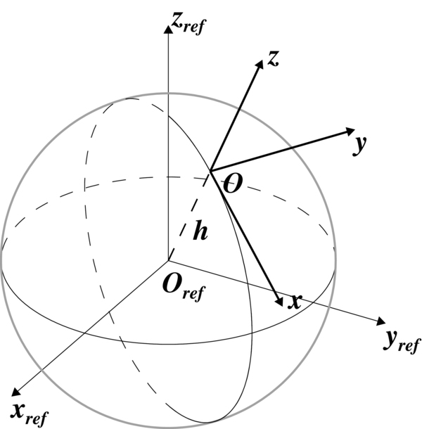
Figure 1. Schematics of coordinate systems. One schematic is the reference coordinate system (xref, yref, zref). Origin, Oref, is located at the solar center and the zref-axis is defined as the solar rotational axis. The xref-axis intersects with the central meridian seen from the Earth. Thick arrows refer to the axes of the local coordinate system (x, y, z). In the local coordinate system, origin O is located at a spherical surface with height h, and the z-axis is defined as the radial direction passing Oref and O. The x-axis is tangent to the longitudinal great circle at O. Dashed lines represent the parts of the lines in the backside of the image plane.
Download figure:
Standard image High-resolution imageFigure 2 shows how we create the ellipsoid model (left) and the GCS model (right) in the coordinate systems defined above. In both panels, the reference coordinate system is shown at the bottom-right corners. To define the ellipsoid model, we use seven geometric parameters: three parameters for the origin of the local coordinate system in the reference coordinate system, OE ( ,
,  ,
,  ) in the Cartesian system or OE (hE, θE, ϕE) in the Spherical system, where hE, θE, and ϕE are height, latitude, and longitude respectively. The other three parameters are for the ellipsoid model, a, b, and c, the length of the three semi-principal axes. The last one is the rotation angle γE around the zE-axis, i.e., the angle between the direction of the principle axis a with respect to the xE-axis. As seen in Figure 2(a), an ellipsoid is determined in the local coordinate system as follows:

where 0° ⩽ μ ⩽ 180° (co-latitude) and 0° ⩽ ν ⩽ 360° (longitude). In case a = b = c, the ellipsoid degenerates into a sphere.

Figure 2. Schematics of the ellipsoid and GCS models. Panel (a) shows the ellipsoid model in the local coordinate system (xE, yE, zE). Parameters a, b, and c are the distances from origin OE to the surface along xE, yE, and zE-axes, respectively. The surface is represented by longitudinal and latitudinal curves. The surface on the zE–xE plane is represented with blue (xE ⩾ 0) and cyan (xE ⩽ 0), and the surface on the yE–zE plane is red (yE ⩾ 0) and orange (yE ⩽ 0). The intersection of the ellipsoid with the xE–yE plane is represented with blue (xE ⩾ 0 and yE ⩾ 0), red (xE ⩽ 0 and yE ⩾ 0), cyan (xE ⩽ 0 and yE ⩽ 0), and orange (xE ⩾ 0 and yE ⩽ 0) colors. Dashed lines represent the parts of the lines in the backside of the image plane. In Figures 5–7, we present the determined ellipsoids in the same way, but the latitudinal circles are on the intersections of the ellipsoids with the solar surface, instead of the xE–yE plane. Panel (b) shows the GCS model in the local coordinate system (xG, yG, zG). In both panels, the origin of the reference coordinate system is located at the bottom-right corners.
Download figure:
Standard image High-resolution imageIn addition to the ellipsoid model, Figure 2(b) shows the GCS model. Note that the local coordinate system could be defined independently for the ellipsoid and the GCS models depending on the shape of CME structures. Subscripts "E" and "G" stand for the terms of ellipsoid and GCS. In order to define the GCS model, we use seven geometric parameters, the origin OG( ,
,  ,
,  ) or OG(hG, θG, ϕG) in the reference coordinate system, half angle α, aspect ratio κ, height H, and rotation angle γG around the zG-axis. We adopt the GCS model in Thernisien et al. (2006) and Thernisien (2011) with two modifications. One modification is that the axis of GCS lies on the x–z plane, not on x–y plane as shown in Thernisien (2011), for the sake of clarity in our compound model. Second, the origin of the GCS model is not necessarily located at the solar center, as shown in Figure 2(b) (more details will be given later). See Thernisien et al. (2006) and Thernisien (2011) for the detailed descriptions of the GCS model.
In practice, the construction of the model is a multiple and iterative process. We make an initial guess of the free parameters and construct the ellipsoid and GCS models in the reference coordinate system. Then, we calculate the viewings of the structure on 2D planes, which correspond to the actual image planes as observed by spacecraft. Then next, through visual inspection, we compare the calculated viewings with the actually observed fronts. To do this, the geometries of the constructed structures in the reference coordinate system are transformed to the observational coordinate systems, (Xsc, Ysc, Zsc), where the subscript "sc" refers to spacecraft that are used. See Kwon et al. (2010) for the explanation of the coordinate transformation method from the reference coordinate system to multiple observational coordinate systems. See also Thompson (2006) and Thompson & Wei (2010) for the detailed explanation of how to use FITS keywords for coordinate systems. As for the observational coordinate systems, the origin Osc is located at the solar disk center in observed images and the Xsc-axis is toward the observer. Ysc and Zsc axes are the westward and northward directions on the image (CCD) plane.
If we could assume that the light paths (to all CCD pixels) are parallel to each other, the transformed coordinates (Ysc, Zsc) correspond directly to the CCD planes (cf. Kwon et al. 2010, 2012). However in this study, our purpose is to reconstruct the large-scale structures in 3D space, thus we should consider the actual light path corresponding to each CCD's pixel. To do this, the coordinates of the constructed 3D structures are transformed to the angular distances (u, v) from the CCD centers in the directions of the west and north of the CCDs, respectively. The angular distances of a point (X', Y', Z') in an observational coordinate system are defined as follows:
where Y'' = Y' − ΔY, Z'' = Z' − ΔZ, and d = D − X'. The parameters ΔY and ΔZ are the offsets between the image center and the solar center on the image plane. In addition, D is the distance of the observer from the Y–Z plane, that is,

where d☉ is the distance of the observer from the solar center. We repeat these processes iteratively until the modeled geometries can represent well the observed features seen from all instruments. Note that we determine the 3D morphology using time series observations, usually assuming the self-similarity with time of the structures. In this context, one of the important constraints to determine the directional geometric parameter is to smooth the variation of the parameters with time. After we determine the 3D morphologies for all time steps, we repeat the fittings until all parameters have smooth variations with time.
3. DATA
The key of this study of the 3D structure is to use observations from multiple viewing perspectives. The Solar Terrestrial RElations Observatory (STEREO; Kaiser et al. 2008) consists of twin spacecraft, named Ahead and Behind, and they move nearly along the Earth orbit followed by and following the Earth, respectively. The two spacecraft provide us simultaneous observations of the Sun from two viewing perspectives. In addition to STEREO, we use the third eye, providing nearly the Earth view, such as from SOlar and Heliospheric Observatory (SOHO; Domingo et al. 1994) and Solar Dynamics Observatory (SDO; Pesnell et al. 2012).
In this paper, we study a CME that occurred on 2012 March 7 and was observed by multiple instruments from four different spacecraft. First of all, we use the Extreme UltraViolet Imager (EUVI; Wülser et al. 2004) of the Sun Earth Connection Coronal and Heliospheric Investigation (SECCHI; Howard et al. 2008) on board STEREO. EUVI provides full-disk imaging observations in EUV passbands, up to 1.7 R☉. We use 195 Å passband images that contain 2048 × 2048 pixels and have a spatial resolution of 1 6. COR1 and COR2 coronagraphs of STEREO SECCHI provide white light observations with fields of view of 1.4–4 R☉ and 3–15 R☉, respectively. The COR1 image contains 512 × 512 pixels and the spatial resolution of the image is 15 The COR2 image contains 2048 × 2048 pixels and the spatial resolution is 15''. We also use 193 Å passband image of the Atmospheric Imaging Assembly (AIA) of SDO, which contains 4096 × 4096 pixels and has a spatial resolution of 06. SOHO Large Angle Spectroscopic COronagraph (LASCO) C2 and C3 coronagraphs (Brueckner et al. 1995) provide white light images of the extended solar corona from 2 to 6 R☉ and from 3.7 to 30 R☉, respectively. The SOHO LASCO C2 image consists of 1024 × 1024 pixels with a spatial resolution of 12''. The image of SOHO LASCO C3 consists of 1024 × 1024 pixels with a spatial resolution of 56''. At the time of the CME of interest occurring, the separation angles of STEREO Ahead and Behind with the Earth were 109° and 118°, respectively, and the three different viewing perspectives provide the observations of any features from all surrounding the solar corona. Table 1 lists all time steps of the observations we analyze.
Table 1. Determined Geometric Parameters of the Ellipsoid Model for All Time Steps We Analyzed
| Time (UT) | θE | ϕE | hE | a | b | c | γE | ||
|---|---|---|---|---|---|---|---|---|---|
| STEREO B | SOHO/SDO | STEREO A | (°) | (°) | (R☉) | (R☉) | (R☉) | (R☉) | (°) |
| 00:10:57e | 00:10:22a | 00:10:52e | 71 | −35 | 1.0 | 0.4 | 0.4 | 0.4 | 30 |
| 00:15:57e | 00:15:25a | 00:15:52e | 71 | −35 | 1.1 | 0.6 | 0.6 | 0.6 | 30 |
| 00:20:26r1 | 00:20:22a | 00:20:21r1 | 69 | −35 | 1.5 | 0.9 | 0.8 | 0.8 | 30 |
| 00:25:26r1 | 00:25:25a | 00:25:21r1 | 66 | −35 | 2.0 | 1.8 | 1.6 | 1.5 | 30 |
| 00:30:26r1 | 00:30:22a | 00:30:21r1 | 65 | −35 | 2.5 | 2.8 | 2.2 | 2.3 | 30 |
| 00:35:26r1 | 00:36:55c2 | 00:35:21r1 | 65 | −35 | 2.9 | 3.7 | 2.8 | 3.0 | 30 |
| 00:39:26r2 | 00:40:22a | 00:39:21r2 | 65 | −35 | 3.2 | 4.4 | 3.4 | 3.6 | 30 |
| 00:50:26r1 | *00:48:54c2 | 00:50:21r1 | 65 | −35 | 4.2 | 5.9 | 4.5 | 4.8 | 30 |
| 00:54:26r2 | 00:54:54c3 | 00:54:21r2 | 65 | −35 | 4.7 | 6.8 | 5.3 | 5.8 | 30 |
| 01:24:26r2 | ... | 01:24:21r2 | 65 | −35 | 6.0 | 11.0 | 9.0 | 11.0 | 30 |
| 01:54:26r2 | 01:54:54c3 | 01:54:21r2 | 65 | −40 | 8.0 | 14.0 | 13.0 | 16.0 | 30 |
Notes. The listed times are the corrected times based on the times in FITS headers, supposing that the spacecraft are located at 1 AU (Astronomical Unit) from the Sun. Since we used composite images, the times correspond to the images of the largest fields of view. θE and ϕE are the latitudes and longitudes of the zE-axis in the reference coordinate system. hE is the heliocentric distance of origin of the local coordinate system, OE. a, b, c, and γE are the geometric parameters of the ellipsoid model defined in the local coordinate system. Superscripts "e," "a," "r1," "r2," "c2," and "c3" refer to the instruments, EUVI, AIA, COR1, COR2, C2, and C3, respectively. We took the corrected time of STEREO Behind as the time of the array of observations, except the time 00:50 (*).
Download table as: ASCIITypeset image
4. RESULTS
Figure 3 shows composite images right before the eruption of the CME event on 2012 March 7, showing the solar corona from the solar disk center to the extended corona up to 6 R☉. The composite images in panels (a) and (c) consist of images taken from EUVI 195 Å, COR1, and COR2 of STEREO Behind and Ahead, respectively. Arrows in these panels point to the outer boundaries of the images of EUVI and COR1. Panel (b) shows the composite image of SDO AIA 193 Å, SOHO LASCO C2, and C3. The three arrows in this panel indicate the boundaries of AIA, the occulting disk of C2, and C3 images. The latitudes and longitudes of the flare site (θsc, ϕsc) are (26°, 81°), (25°, −37°), and (25°, −146°) in the three observational coordinate systems of EUVI of STEREO Behind, AIA of SDO, and EUVI of STEREO Ahead, respectively; a plus symbol in each panel refers to the flare site. In the case of the observations of STEREO Ahead in panel (c), the flare site is located on the back side of the Sun. Since each spacecraft observed the Sun at a different distance, we corrected the time in the FITS header of raw image files, supposing that each spacecraft is located at the distance of 1 AU (Astronomical Unit) from the solar center. At the bottom-left corner of each panel, the corrected time of the image of the largest field of view is given. The time in the FITS header is also given in parenthesis. The corrected times of the images taken from STEREO Behind serve as the time of events observed from the three different viewing perspectives.

Figure 3. Composite images showing the solar corona from the solar disk center to the extended corona up to 6 R☉, observed from STEREO Behind (a), SOHO and SDO (b), and STEREO Ahead spacecraft (c). At this time, the separation angles of STEREO Behind and Ahead spacecraft with the Earth are 118° and 110°, respectively. Panel (a) consists of images taken from EUVI 195 Å, COR1, and COR2 of STEREO Behind. Panel (b) shows the composite image of SDO AIA 193 Å, SOHO LASCO C2, and C3. Panel (c) shows the composite image of EUVI 195 Å, COR1, and COR2 of STEREO Ahead. The black circle in each panel represents the solar disk. In panels (a) and (c), arrows denote the outer boundaries of images taken from different instruments, EUVI and COR1. In panel (b), three arrows indicate the boundaries of AIA, the occulting disk of C2, and C3. A plus symbol in each panel refers to the flare site on the solar surface. In the case of panel (c), the flare site is located on the back side of the Sun and the site is represented with a black plus symbol. The latitudes and longitudes of the flare site (θsc, ϕsc) are (26°, 81°), (25°, −37°), and (25°, −146°) in the three observational coordinate systems of EUVI of STEREO Behind, AIA of SDO, and EUVI of STEREO Ahead, respectively. The time at the bottom-left corner of each panel shows the corrected time of the observation having the largest field of view. The time in the FITS header is also given in parenthesis. A composite image is synthesized by images of the closest times.
Download figure:
Standard image High-resolution imageFigures 4 and 5 show selected time series observations of the CME. Three columns show the different perspectives of the event observed from STEREO Behind (left), SOHO/SDO (middle), and STEREO Ahead (right). While the white light observations in Figure 4 are shown as intensity images, Figure 5 provides their running difference images with our fitting results. Thanks to the three viewing perspectives, the combined observations show nearly the side view, top view, and bottom view of the CME, thus the full 3D structure from the footprints to the leading fronts.
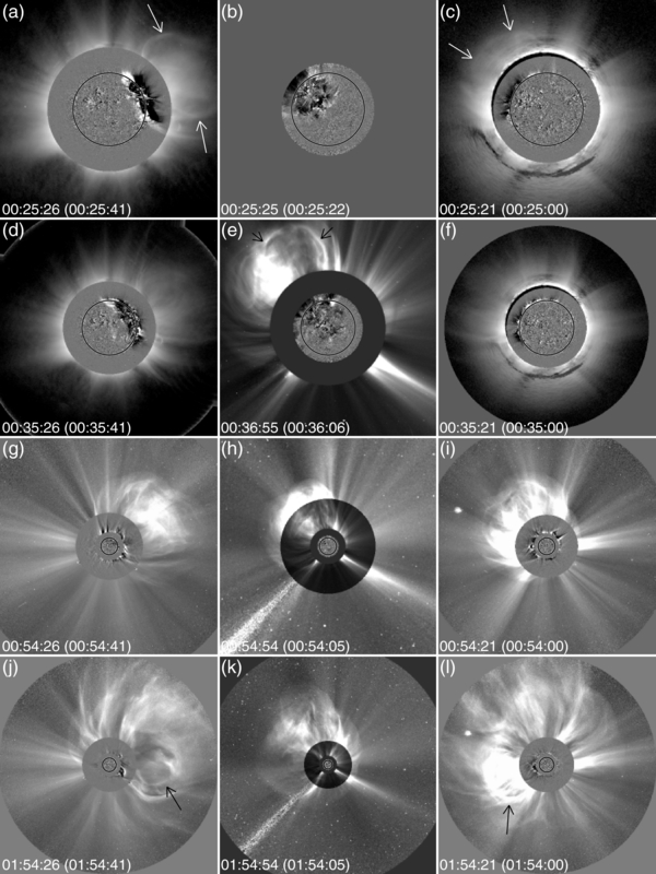
Figure 4. Selected time series observations of the analyzed CME on 2012 March 7. Left, middle, and right columns show the composite images observed from STEREO Behind, SDO and SOHO, and STEREO Ahead, respectively. The solar center is located at the center of each panel, and the solar rotational axis is the north of each image. The black circle in each panel refers to the solar disk. Panels (a)–(c) show the solar corona from the solar center to 3 R☉, (d)–(f) are 4 R☉, and (g)–(i) are 13 R☉. Panels (j) and (l) show the solar corona up to 18 R☉, and panel (k) shows the solar corona up to 30 R☉. The images of EUVI 195 Å are the running difference images, and the images of AIA 193 Å are the running ratio images. White light observations are presented as the intensity images. Dark gray parts in panels (b) and (f) are the regions where the corresponding observations are not available at those time steps. The time at the bottom-left corner of each panel shows the corrected time (FITS header time) of the observations of the largest fields of view.
Download figure:
Standard image High-resolution imageFigure 5. Representations of the constructed 3D structures of the CME on 2012 March 7 as observed over the time series as seen in Figure 4. Different from Figure 4, white light images are shown as the running difference images. Yellow curves represent the ejecta front with the GCS model, and the others represent the outermost front with the ellipsoid model. All time steps of observations and the fitting results are available as Movie 1 in the online journal: left, middle, and right panels show the composite images taken from STEREO Behind, SDO and SOHO, and STEREO Ahead, respectively. Top panels show the intensity images, while bottom panels show the running difference or running ratio (AIA) images. The time at the bottom of each top panel shows the corrected time of the images of the largest field of view.
(An animation and a color version of this figure are available in the online journal.)
Download figure:
Video Standard image High-resolution imageThe top panels in Figures 4 and 5 show the corona up to 2 R☉. The CME in Figure 4(a) appears as the typical three-part structure—the bright frontal loop (arrows), the dark cavity, and the bright core. On the other hand, in Figure 4(c), the three-part structure is not clear but rather a looplike front, possibly the bright frontal loop, is seen (arrows). The bright frontal loop on COR1 image in panel (a) seems to have the trailing edges that are connected to the dark region of the running difference image of EUVI Behind, implying that the bright frontal loop has the legs rooted on the dimming region. In the running difference images of EUVI and AIA shown in panels (a) and (b), the EUV wave front emerges outside of the dimming region and the EUV wave front in Figure 5(a) seems to be connected to the outermost front in the extended solar corona observed with COR1 Behind. In Figure 4(b), the size of the CME is still small enough that the CME is not observed in LASCO C2 at this time. The images of COR1 Behind (in panels (a) in Figures 4 and 5) and Ahead (in panels (c) in the figures) show that the trailing edges of the bright frontal loop interact with streamers.
Panels (a)–(c) in Figure 5 show the representations of the outermost front and the bright frontal loop of the CME with the ellipsoid and GCS models, over the observed images. The determined GCS model is represented by yellow curves, and the outermost front is denoted by white, blue, red, cyan, and orange colors, as seen in Figure 2(a). At this time step, LASCO C2 is not available, so we fitted the GCS model to the bright frontal loop observed by COR1 Behind and Ahead, which is denoted by arrows. In the intensity images in Figure 4 and the running difference images in Figure 5, it is seen that the coronal streamers adjacent to the CME fronts are deflected. In addition, the outermost front is extended to the ambient corona in the azimuthal direction more than that of the bright frontal loop. In contrast, we were not able to find the difference in the height of the two fronts. Through the iterative fittings, we found that the outermost front is reproduced well with an oblate spheroid (a = b and a > c).
Panels (d)–(f) in Figures 4 and 5 show composite images with a field of view of 4 R☉. Figure 4(e) shows the most part of the CME, and the CME is observed as the bright frontal loop, cavity-like dark region, and corelike bright region. In comparison with Figure 3(b), the corelike bright region may be the preexisting streamer deflected by the CME. Using the bright frontal loop in panel (e) and the part of the trailing edges seen in panels (d) and (f), we determined the geometric parameters of the GCS model. Figures 5(d)–(f) show the best fit of the GCS model. As for the fuzzy outermost front, we found that a > b and a > c. It is interesting to note that a ≠ b, unlike that in the previous time step.
The field of view of composite images in panels (g)–(i) in Figures 4 and 5 is 13 R☉. Different from the previous time steps, the outermost front and the bright frontal loop are clearly separated in all directions (see Figure 9(a)). On the other hand, similar to the two previous time steps, the bright frontal loop seems to be connected to the solar surface through the lower solar corona observed with COR1 and EUVI of STEREO Behind (Figure 4(g)). It is interesting to note that the shape of the outermost front is best approximated to a sphere (a ∼ b ∼ c), and the bottom part of the sphere does not intersect with the solar surface anymore.
Panels (j)–(l) in Figures 4 and 5 show composite images with the full fields of view of COR2 (15 R☉) and C3 (30 R☉). There was another CME occurred at ∼01:05 (UT) and the newly outgoing CME is seen in panels (j) and (l), but close to the Sun (arrows). At this time step, the outermost front and the bright frontal loop are much larger than the ones in the previous time steps and may be larger than the field of view of COR2. Since the bright frontal loop cannot be clearly seen in the images of this time step, we did not reproduce the bright frontal loop. As for the outermost front, LASCO C3 shows the whole structure appearing as a full halo shape, and the COR2 Behind and Ahead images show the lateral and the rear part of the structure, respectively. Different from the previous steps, the geometric parameter c is now larger than a and b, resulting in a prolate shape (c > a ∼ b). Movie 1 shows the animation of the observations and measurements in all time steps.
Figure 6 shows EUV observations of STEREO EUVI Behind (left panels) and SDO AIA (right) in the initial stage of the CME. The CME is observed as expanding loops in EUVI images, and the top part is shown in COR1 observations, simultaneously. This leading front is observed to be the bright frontal loop in the later white light observations (see Movie 1). The expanding loops in the EUVI image and the leading bright front in the COR1 image are represented with a single GCS model as shown in panel (c). At this time step, we were not able to find the orientation of the GCS model because we have only one viewing perspective from STEREO Behind, so we simply used the same orientation determined on the next time step. As for the outermost front, the running difference of the EUVI image and the running ratio of the AIA image bring out a fuzzy and extended front that runs ahead of the expanding bright frontal loop in the lateral direction, as shown in panel (c). In the radial direction, the difference in height of the two fronts is small enough to be noticed.

Figure 6. Simultaneous observations of the CME on 2012 March 7 by EUVI 195 Å of STEREO Behind and AIA 193 Å of SDO at 00:15 UT. Top panels show the intensity images of EUVI (a) and AIA (b), and bottom panels are the running difference and the running ratio images, respectively, with determined shapes of the ellipsoid and GCS models. In the bottom-left corners, the simultaneous STEREO COR1 Behind observation is given as the intensity (a) and the running difference image (c). The two arrows in the EUVI images point at the lateral flanks of expanding loops, and an arrow in COR1 images points at the front presumed to be the top part of the expanding loops. The corrected times (FITS header times) of the images are given in top panels. See the text for detailed descriptions.
Download figure:
Standard image High-resolution imageFigure 7 shows the solar disk observed with EUVI 195 Å Behind (running different images; left panels) and SDO AIA 193 Å (running ratio images; right panels). The representations of the outermost front and the bright frontal loop are overplotted in the same way as seen in Figures 4 and 5. But now, this Figure clearly shows the intersection of the determined ellipsoids with the solar surface. It is found that, spatially, the intersection of the ellipsoid coincides well with the EUV wave front. The EUV observations and the fitting results of all time steps are available in Movie 2.
Figure 7. Selected time series observations of the CME on 2012 March 7 by EUVI 195 Å of STEREO Behind and AIA 193 Å of SDO. Left and right panels show the running difference and running ratio images of EUVI and AIA, respectively. The corrected times (FITS header times) of the images are given at bottom-left corners. Panels (a), (b), (c), and (d) correspond to panels (a), (b), (d), and (e) in Figures 4 and 5, respectively. The determined shapes of the ellipsoid and GCS models are presented in the same way as in Figure 5. All time steps of EUV observations and the fitting results are available as Movie 2 in the online journal left, middle, and right panels show the running difference/ratio images of EUVI 195 Å of STEREO Behind, AIA 193 Å of SDO, and EUVI 195 Å of STEREO Ahead, respectively.
(An animation and a color version of this figure are available in the online journal.)
Download figure:
Video Standard image High-resolution imageTo characterize the evolution of the outermost front of the CME, Figure 8 shows the variation of the geometric parameters of the ellipsoid model. From top to the bottom, these panels show the parameters, the height of the center of the ellipsoid (hE), a, b, c, and ratios of the geometric parameters, c/a (circle symbols), and a/b (diamond symbols). Error bars in panels (a)–(d) show the errors in the parameters, which are estimated to be ± 8% of the determined values (see Appendix). Error bars in panel (e) represent the propagation errors calculated with the errors in a, b, and c. These values are also listed in Table 1. Panel (e) shows a geometric characteristic of the outermost front. The ratio, c/a shows the shape of the cross-section of the ellipsoid on the xE–zE plane, while the ratio a/b shows the cross-section on the xE–yE plane. At the beginning stage of the CME, the ellipsoid is found to be almost a sphere. As time goes by, the parameter a increases at a faster rate than the one of c. Around 01:20 UT, the cross-section becomes a circle again. It then evolves into an ellipsoid of a < c. Similarly, the cross-section on the xE–yE plane starts as a circle, but the increase rate of a is faster than b. The ratio increases until ∼00:40 UT and then starts to decrease.
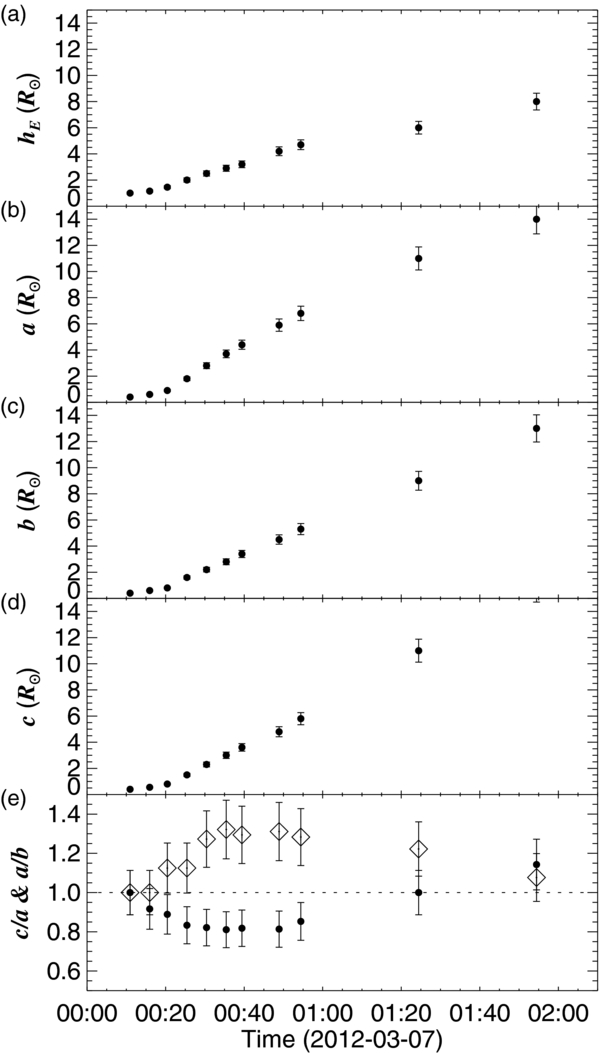
Figure 8. Geometric parameters of the ellipsoid model representing the outermost front of the CME. The panel (a) shows the height of the center of ellipsoid (hE). Panels (b)–(d) show the lengths of the three semi-principal axes, a, b, and c, respectively. Panel (e) shows the ratios of c with a (filled circles) and a with b (diamonds).
Download figure:
Standard image High-resolution imageFigure 9 shows the geometric characteristics of the bright frontal loop determined with the GCS model. The error in the GCS model is estimated to be ± 7% of the determined structure (see Appendix). Panel (a) shows the heights of the leading edge of the GCS with open circles; as a comparison, the heights of the leading edge of the ellipsoids are shown with filled circles. Panel (b) shows the widths of the GCS model (open circles) and the ellipsoid model (filled circles). The heights of the leading edge of the GCS model were derived from the sum of the height of the origin, hG, and the height of the GCS, H. In the case of the ellipsoid model, the heights of the leading edge were determined by the sum of the heights of the origin, hE, and parameter c. The difference in heights of the two leading edges ΔH are presented in panel (d) with error bars. As seen in panels (a) and (d), the two leading edges are very close to each other in the beginning, and they appeared apparently detached only after 00:30 UT. Considering the error bars, we could not conclude that the heights of the two leading edges are different in the first three data points in panel (d). The error bar of the fourth point at 00:30 UT implies that the difference now became noticeable. It is interesting to note that ΔH tends to increase with time, which is consistent with previous results on the standoff distances (e.g., Gopalswamy & Yashiro 2011; Gopalswamy et al. 2012; Poomvises et al. 2012). In a simple geometry, the difference in height ΔH is proportional to the standoff distance between a shock front and the driver. The width of the GCS model can be determined by the half maximum separation of the GCS model, while the width of the ellipsoid model can be determined from the parameter a. Panel (e) shows the difference in width of the GCS model and the ellipsoid model. It is evident as shown in panel (e) that the two fronts were detached immediately in the beginning of the eruption. The difference in width is much larger than that in height.
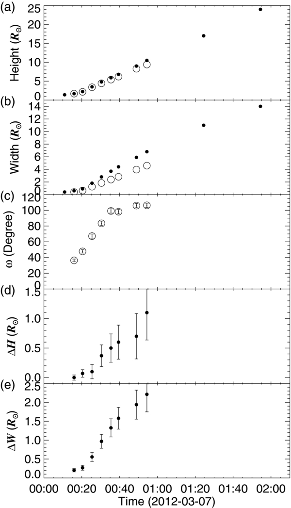
Figure 9. Geometric characteristics of the bright frontal loop represented with the GCS model and comparisons with the ones of the outermost fronts determined with the ellipsoid model. Since we focused on the outlines of the bright frontal loop, rather than the internal structures, we present the geometric characteristics of the outlines of the bright frontal loop, such as height of the leading edge determined as hG+H (a), the half width (b), and the angular width defined as the separation angle of the full width at the solar center (c). In panels (a) and (b), the height of the ellipsoid determined as hE+c and geometric parameter a is given, respectively, as filled circles for the comparisons. In these panels, the error bars are omitted from the plots for the comparisons. Panel (d) shows the differences between the two heights shown in panel (a). Panel (e) shows the differences between the two half widths shown in panel (b).
Download figure:
Standard image High-resolution imageFigure 10 shows the velocity evolution of the two leading fronts determined from the GCS model (open circles) and the ellipsoid model (filled circles). In panel (a), we show the velocity along the radial direction, while in panel (b) we show the velocity along the lateral direction. The solid curve in panel (a) shows a temporal profile of the GOES X-ray flux that indicates the flare. The velocities along the radial direction were derived from the height measurement in Figure 9(a), while those along the lateral direction were determined from the results in Figure 9(b). In both cases, the significant acceleration occurred during the rise phase of the GOES X-ray flare. It is interesting to note that the velocities of the two fronts along the radial direction are identical, considering the error bars. On the other hand, the velocities of the two fronts along the lateral direction are significantly different. After 00:20 UT, the outermost front is more than 500 km s−1 faster than the bright frontal loop along the lateral direction, indicating the different nature of the two fronts.

Figure 10. Speeds of the outermost front and the bright frontal loop determined with the ellipsoid and GCS models. Panel (a) shows speeds of the leading edges of the outermost front (filled circles) and the bright frontal loop (open circles) in the radial direction. On the other hand, panel (b) shows speeds of the leading edges of the outermost front and the bright frontal loop in the lateral direction. The solid curve in panel (a) refers to a GOES X-ray flux.
Download figure:
Standard image High-resolution imageThe sketch in Figure 11 summarizes the determined 3D morphology of the outermost front and the bright frontal loop in the viewing perspective of STEREO Behind. In the initial stage, the leading front of the bright frontal loop is very close to that of the outermost front. However, the distance between the two fronts increases with time. In contrast, in the lateral direction, the two fronts are separated well from the initial stage. The outermost front in the initial stage is close to a sphere in shape, then it appears as a squashed ellipsoid (approximated to an oblate), and then it evolves into an elongated ellipsoid (approximated to a prolate) at the last time step we analyzed. Contrary to the bright frontal loop, the outermost front propagates in all directions above the solar surface. As it expands in all directions, the ellipsoid intersects with the solar surface, forming the footprint that is observed as the EUV wave front in the EUV images. Eventually, the ellipsoid becomes large enough and does not intersect with the solar surface anymore, but encloses the whole solar corona (see also Movie 3).
Figure 11. Temporal evolutions of the outermost front and the bright frontal loop determined with the ellipsoid and GCS models, respectively. This illustration shows the STEREO Behind views. A circle with a black solid line refers to the solar disk. Gray solid lines followed by yellow solid lines show the outlines of ellipsoids representing the outermost fronts. The yellow solid lines refer to the bright frontal loop determined with the GCS model. These outlines are taken from the observations at 00:25, 00:35, 00:54, and 01:54 (UT). The outline of an ellipsoid determined at 01:54 (UT) is much bigger than this image, so that the only part of the outline is shown in the bottom-left and top-left corners of this figure. Dotted circles represent the heliocentric distance from the solar center at 4, 8, and 12 R☉ on the image plane. The temporal evolutions of the 3D morphologies are also available as Movie 3 in the online journal: A circle in each panel represents the solar disk. The three panels have been made, assuming that the observers are located at (0, −1 AU, 0), (1 AU, 0, 0), and (0, 0, 1 AU), where AU is the Astronomical Unit, in the reference coordinate system. By the definition, the middle panel shows the Earth view of the temporal evolutions of the 3D morphologies.
(An animation and a color version of this figure are available in the online journal.)
Download figure:
Video Standard image High-resolution image5. DISCUSSION
5.1. Insights into the Nature of CMEs
By applying our compound geometric model (consisting of both the ellipsoid and the GCS models) to the CME event observed from the three different viewing perspectives, we revealed the presence of two distinct CME fronts: the outermost front (faint front of diffuse emission) that can be well reproduced with the ellipsoid model, and the bright frontal loop (in a classical three-part structure) that can be reproduced with the GCS model. The simultaneous fitting of the two fronts with the two distinct geometries demonstrates that they are not the projection of a single 3D structure in the plane of the sky, but they have an intrinsically different 3D morphology.
To date, it has been thought that identifying shock waves in white light observations is very difficult or impossible because of the lack of knowledge about magnetic field topology and density in the corona (Ciaravella et al. 2006; Webb & Howard 2012; Vourlidas et al. 2013). However, Kwon et al. (2013b) pointed out that coronal streamers are the proxy of the global magnetic separatrix. While the trailing edges of the underlying magnetic structure could not pass through the open magnetic field lines observed as coronal streamers, the fast magnetosonic shock wave fronts may pass freely through the open magnetic field lines. The bright frontal loop is found to have the fixed legs rooted on the solar surface, and their trailing edges are found to be confined to a region surrounded by coronal streamers as they move outward. On the other hand, the outermost front is found to pass through the surrounding deflected coronal streamers. The EUV wave front is found to be the footprint of the outermost front. These facts indicate that the outermost front is in fact a fast magnetosonic shock wave front, while the bright frontal loop is the outline of the underlying magnetic structure, possibly a magnetic flux rope.
It is interesting to note that the 3D morphology of the shock wave (the outermost front) can be well represented by the ellipsoid model. It has been regarded that the outermost front is a bow-shock with the shape of a hyperbolic surface (e.g., Vourlidas et al. 2013). It is obvious that, while the hyperbolic surface may reproduce well the top part of the outermost front, it is difficult to explain the lower part that is connected to the EUV wave front. Furthermore, the shock wave front is seen to propagate in all directions above the solar surface, even in the opposite direction of the CME propagation, as pointed by arrows in Figures 5(j) and (k). Our results highly suggest that the 3D shape of the fast magnetosonic shock wave front is a bubble that could be fairly reproduced with the ellipsoid model.
Note that the hyperbolic surface and the bubble-shaped front are not mutually exclusive. Associated with flares and/or CMEs, there may be two shock formation mechanisms (e.g., Vršnak & Cliver 2008). One mechanism is the bow-shock in that a shock propagates ahead of the driver in the shape of a hyperbolic surface and the speed of the shock is equal to that of the driver. The other is the piston-shock in that the shock speed is faster than that of the driver. In this case, a wave is driven to propagate freely in all directions in the shape of a bubble. Interestingly, our results show both characteristics simultaneously. Figure 10 shows the speeds of the outermost front (filled circles) and the bright frontal loop (open circles) in the radial direction in panel (a) and in the lateral direction in panel (b). While the speeds in the lateral direction are significantly different from each other, the difference in speeds in the radial direction is considerably small, or the same within the error bars. These facts demonstrate that the observed shock wave front could be associated with the piston-shock in all directions and the bow-shock in the radial direction. In this case, the leading edge of the CME ejecta would catch up with the wave bubble ahead in the radial direction and modify the shape of the wave bubble.
This idea is consistent with the shock theory and the accepted evolution history of CMEs. It has been known that the expansion is dominant in the initial phase, and then the outward motion in the radial direction becomes dominant in the later phase (e.g., Patsourakos et al. 2010). The rapid and temporary expansion in the initial phase may result in the piston-shock, while the persisting radial motion of the CME ejecta may be responsible for the bow-shock. Note that the CME we studied here shows the general evolutionary history; the rapid acceleration (Figure 10(a)) and expansion (Figure 10(b)) of the bubble-shaped wave and the bright frontal loop all occurred during the impulsive phase of the flare (Zhang et al. 2001).
In the case that a freely propagating fast magnetosonic wave is driven from a pointlike source in a homogeneous medium, the wave front will propagate in all directions and the shape will be a sphere, supposing the Alfvén speed is much larger than the sound speed. However, in reality, the coronal medium is highly inhomogeneous (e.g., Kwon et al. 2013a). Even if a wave is triggered to propagate in all directions, the solar surface will interrupt its spherical expansion and the wave front would be found only above the source region. At this point, a question naturally arises of how the wave propagates to the opposite side of the Sun, sweeping the solar surface and then becoming such a big bubble enclosing the Sun, as shown in Figures 5(j)–(l). There is an important characteristic of coronal medium that may allow us to answer to the question; the local fast magnetosonic speed in quiet Sun and coronal holes increases with height in the low solar corona until a certain height (3–4 R☉) and then starts to decrease (Gopalswamy et al. 2001; Mann et al. 2003; Evans et al. 2008; Kwon et al. 2013a, 2013b). The increasing local fast magnetosonic speed in the low corona would result in the wave refraction toward the solar surface, and then the refracted wave would form the front that faces the opposite side of the source region, as seen in Figure 11 (see also, Figure 4 in Uchida 1968).
5.2. Insights into EUV and Moreton Waves
To date, the co-moving EUV waves with the lateral flanks of CMEs have been often interpreted as the footprints of the stretched magnetic field lines overlying expanding CME flux rope (Chen et al. 2002; Chen 2009; Dai et al. 2010; Warmuth & Mann 2011) or successive magnetic reconnections (Attrill et al. 2007). These interpretations may be because all observed lateral flanks of CMEs have been simply presumed to be the trailing edges of the expanding flux rope or the stretched magnetic field lines. However, we found that the co-moving "lateral flank" is the bubble-shaped fast magnetosonic shock wave.
Our results imply that EUV waves are a bubble-shaped 3D phenomenon (Cheng et al. 2012; Liu et al. 2012; Kwon et al. 2013b), rather than a circular-shaped 2D phenomenon propagating in a specific atmospheric layer. Patsourakos et al. (2009) estimated the height of an EUV wave front using a triangulation method and concluded that the EUV wave propagates in the low coronal layer with a height of about 90 Mm, which is comparable to the coronal scale height. Note that, however, this result could be explained by an alternative way; the lower part of a bubble-shaped wave front within the coronal scale height would be observed effectively in the EUV passbands because of the dense medium. When the refracted wave front passes through the dense coronal medium within the coronal scale height, the wave front would be shocked and observed as the EUV wave in the EUV passbands. In case the energy of the refracted wave is enough to reach the chromosphere through the low coronal medium, the wave will be shocked in the chromosphere and observed as a Moreton wave in Hα observations. It may be the reason why Moreton waves are observed to propagate in shorter distances than the associated EUV waves (Warmuth et. al 2004; Asai et al. 2012).
5.3. Insights into Halo CMEs
Our results and interpretations above may reconcile the conflicting conclusions on the general morphology of CMEs. Halo CMEs have been thought to be the CMEs that are traveling nearly along the lines of sight (e.g., Howard et al. 1982). The difference in the morphologies between halo CMEs and the other classes of CMEs has been believed to be only due to the viewing perspectives without any differences in the physical nature. However, the circular shape of halo CMEs implies that CMEs are in the shape of a bubble (Howard et al. 1982; Crifo et al. 1983; Sheeley et al. 1999; Michałek et al. 2003; Xie et al. 2004; Xue et al. 2005) while at the same time, the 3D structure of CMEs has been often thought to be a flux rope (Mouschovias & Poland 1978; Munro et al. 1979; Pneuman 1980; Chen et al. 1997, 2000; Thernisien et al. 2006, 2009) because of observations of the bright frontal loop or three-part structure. As we discussed above, the bubble-shaped structure implies that the physical nature of CMEs is a fast magnetosonic shock wave (Steinolfson & Nakagawa 1977; Wu et al. 1983; Vourlidas et al. 2013), while the flux rope-shaped structure indicates that the observed fronts are formed by mass carried by erupting magnetic structure. Because of these conflicting morphologies and the inferred physical nature from the morphologies, the general 3D structure of CMEs and the physical nature have had different interpretations in the past.
The CME we analyzed here has been recorded as a halo CME in the SOHO LASCO CME catalog (Yashiro et al. 2004). Note that this CME appears as a halo CME from all viewing perspectives, as seen in Figures 5(g)–(l). Furthermore, the fronts seen as a halo CME are the ones observed as the outermost front, which is found to be a fast magnetosonic wave front. Figure 11 shows how the bubble-shaped wave front could be observed as the circular front surrounding the solar disk (or occulting disk), even if the viewing perspective is normal to the direction of the CME propagation. The wave front propagates in all directions, even in the opposite direction of the CME propagation, and forms a circular front surrounding the solar disk at 00:54 UT and the occulting disk at 01:54 UT. At 01:54 UT, the bubble-shaped wave front would be observed as a halo CME from all viewing perspectives, covering all around the Sun.
Note that the flux rope can propagate only in the radial direction with the expansion and cannot form a front on the opposite side of the Sun. In case the propagating direction is nearly along a viewing direction, the mass carried by the flux rope may be observed as an elongated shape in the image plane, rather than the circular shape, as shown in middle panels in Figure 5. Furthermore, the mass far ahead of the Sun could not be well observed with white light observations, since Thomson scattering gives the most effective result when the electrons lie on the plane of the sky, that is the Ysc–Zsc plane in our definition. On the other hand, in the same situation, the rear side of the bubble-shaped wave can intersect with the plane of the sky and the cross-section would be observed through Thomson scattering as the circular front of a halo CME.
Dash-dotted curves in Figures 5(j)–(l) refer to the cross-sections of the bubble-shaped wave front in the planes of the sky. While the outlines of the bubble-shaped wave front (solid or dashed curves) are close to the cross-sections in the planes of the sky of STEREO Behind (Figure 5(j)) and Ahead (Figure 5(l)), the outline seen from SOHO (Figure 5(k)) is significantly larger than the cross-section because the outline of the bubble-shaped wave is far ahead of the cross-section. Note that the cross-section is closer to the observed bright circular fronts than the outline of the bubble-shaped wave, suggesting that the scattering light mostly comes from the plane of the sky. This idea is supported by a study of CME fronts with ultraviolet spectra in Ciaravella et al. (2006). They found that Doppler speeds of halo CME fronts are significantly slower than the speeds of the fronts in the planes of the sky and concluded that the fronts may be a shock or a compression wave.
It is interesting to note that above discussions imply that only the CMEs associated with bubble-shaped fast magnetosonic waves could be seen as full halo CMEs, regardless of the propagating direction. On the other hand, the CMEs propagating toward the observers without the wave fronts would not be observed as full halo CMEs. This interpretation may explain the discrepancy between average speeds of halo CMEs and the other CMEs, found by statistical studies in Yashiro et al. (2004); the average speed of halo CMEs is found to be 957 km s−1 and is much faster than that of the other CMEs, which is found to be 428 km s−1. In addition, they found that wide CMEs tend to have high speeds. These facts may be because it is highly possible that high speed CMEs are accompanied by bubble-shaped fast magnetosonic shock wave fronts and these CMEs would be observed as the wider CMEs.
5.4. Insights into Lateral Flanks of CMEs
This work may help clarify what we have seen from white light observations associated with a CME. In particular, it may provide answers to questions such as: What is the physical nature of lateral flank of a CME? And what is the angular width? According to our results, first of all, white light observations of CMEs may show outgoing mass and a freely propagating fast magnetosonic wave front, simultaneously. These two fronts interact with the ambient magnetic structures, coronal streamers, and thus the deflected coronal streamers may be one of the prominent features of running difference images of white light observations. In this context, the lateral flanks of a CME could be the mass carried outward by an expanding flux rope, the wave front, or the deflected streamers. Next, we found that the angular width of the bright frontal loop is about 120°, while the angular width of the outermost front is 360°. To date, it has not been clear what the angular width of CME is, while the angular width is thought to be an important factor for type II radio bursts and gradual solar energetic particle events (e.g., Gopalswamy et al. 2001; Kahler et al. 2003). Since the angular widths have been usually determined as the maximum separation angles of CMEs on the image planes, the angular widths may be the widths of the bubbled-shaped fast magnetosonic waves, when the CMEs are associated with fast magnetosonic waves.
6. SUMMARY AND CONCLUSION
To date, the morphology of CMEs has not been fully understood. In order to reconcile conflicting interpretations of the observations of CMEs within the framework of the 3D structure, we developed a compound model and applied the model to complementary data sets of a CME event on 2012 March 7, obtained from STEREO Behind, SOHO and SDO, and STEREO Ahead. The data sets provide observations of the solar corona from the coronal base to the extended corona up to 30 R☉ with three different viewing perspectives. Associated with the event, EUV images taken from EUVI 195 Å of STEREO Behind and AIA 193 Å of SDO showed the impulsive brightening of the flare and circularly propagating EUV wave. In particular, EUVI observations of STEREO Behind showed a dome-shaped front followed by expanding loops. White light images taken from COR1/COR2 of STEREO and C2/C3 of SOHO showed a faint front of diffuse emission, which is observed to compose the outermost front of the observed CME. In addition to the outermost front, the bright frontal loop was observed as the outline of the three-part structure, following the outermost front. As these multiple fronts were expanding and propagating outward, coronal streamers were deflected.
From the fittings, we found that the outermost front (faint front of diffuse emission) in white light observations and the EUV wave front in EUV observations are represented well with a single ellipsoid model, implying that the outermost front of the CME is a bubble-shaped structure. On the other hand, the expanding loops in EUV observations and the bright frontal loop in white light observations were found to be represented well with the GCS model, suggesting that the CME ejecta front is a flux rope-shaped structure. Our results may provide new insights into the nature of CMEs and the associated shock waves as follows.
- 1.Morphology. A CME could comprise two distinct structures, the outermost bubble and the internal flux rope, forming the observed outer and inner fronts of a CME, respectively.
- 2.Nature. The front observed as the outermost front is in fact a fast magnetosonic shock wave front, while the front observed as the bright frontal loop is the mass carried by flux rope. In other words, the bubble-shaped morphology of CMEs refers to the aspect of the fast magnetosonic wave, and the flux rope-shaped morphology indicates the aspect of the mass carried by flux rope.
- 3.Shock formation mechanism. The observed shock wave could be associated with two different shock formation mechanisms: the piston-shock and the bow-shock. A freely propagating wave is driven in the form of the piston-shock in the initial stage of a CME. The wave propagates in all directions with refractions and forms the bubble-shaped front observed as the outermost front. The bright frontal loop propagates mainly in the radial direction, while its expansion is restricted by the adjacent coronal streamers and then the bow-shock is triggered to propagate with the driver (the leading edge of the bright frontal loop) in the radial direction.
- 4.EUV wave. EUV wave is the footprint of the bubble-shaped fast magnetosonic shock wave, which is refracted toward the solar surface.
- 5.Halo CME. The circular fronts surrounding occulting disks of white light images are the observations of the bubble-shaped fast magnetosonic shock wave, rather than the projection of the three-part structure.
In this paper, we presented the 3D morphology of a CME and the temporal evolution. While we may expect that the overall geometric characteristic, such as the relationship among the outermost front, bright frontal loop, and EUV wave front, is more or less a general feature of CMEs accompanied by the "two-front" morphology, the detailed geometric characteristics, such as the shapes (e.g., ratios of the geometric parameters of the models) and kinematics of the two fronts, may vary depending on certain conditions. In this context, it needs to be extended to a large number of events in order to study and generalize the detailed morphology, kinematics, and nature of CMEs and driven shock waves.
We are grateful to the referee for the constructive comments that helped to improve the manuscript. This work is supported by NSF ATM-0748003 and NSF AGS-1156120. SDO is a mission of NASAs Living With a Star Program. The AIA data used here are courtesy of SDO (NASA) and the AIA consortium. The SECCHI data are produced by an international consortium of the NRL, LMSAL and NASA GSFC (USA), RAL and Univ. Bham (UK), MPS (Germany), CSL (Belgium), IOTA and IAS (France). SOHO is a project of international cooperation between ESA and NASA. The SOHO/LASCO data are produced by a consortium of the Naval Research Laboratory (USA), Max-Planck-Institute für Aeronomie (Germany), Laboratoire d'Astronomie Spatiale (France), and the University of Birmingham (UK).
APPENDIX: ERROR IN 3D GEOMETRY
The uncertainty in the 3D geometry of CMEs and driven shock waves may be mostly caused by the fact that the true shapes of a CME and driven wave are different from the geometric models. This uncertainty may be much larger than the measurement errors caused by resolution, point spread function, and signal-to-noise ratio of images, as shown in Figure 12. In this figure, ellipses refer to the modeled outermost front projected on image planes, and plus symbols represent the actual location of the front. In this work, we are only interested in the error in the overall shape of the modeled structures, rather than the geometric parameters of the models. Basically, the error in the modeled geometry at ith point in 3D space can be defined as

where xi and xmodel, i are coordinates of the true and modeled position in 3D space, respectively. Since the true 3D coordinates xi(xi, yi, zi) are unknown, the error would be estimated in 2D planes, approximately. In this context, the error can be determined with the true and modeled 3D structure projected on a 2D plane, namely,

where λj and λmodel, j are the distances of the points from the geometric center of points consisting of λmodel on the 2D plane. Figure 12 shows how δj can be estimated in the observed image planes. An ellipse represents the series of the points, λmodel, j, on each image plane, and the center of radial lines is the geometric center of λmodel. As a matter of fact, Equation (A2) gives an approximation of δj projected on a 2D plane, rather than the actual error in 3D space. Note that, however, the error determined in 2D planes may let us know how well the model represents the actual 3D structure. We define a ratio,  , by taking an average of the ratios of δj to λmodel, j, considering all observed image planes.
where N is the total number of the points and the subscript k refers to the observed image plane. In this way, the error at jth point on an arbitrary 2D plane can be written as

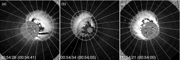
Figure 12. Differences between the modeled outermost front and the observed outermost front from the three different perspectives. Each panel shows the same composite image shown in panels (g), (h), and (i) in Figures 4 and 5, respectively. The solid ellipse in each panel refers to the outline of the modeled outermost front, and plus symbols are the observed outermost front. The plus symbols are nearly on solid lines that spread out radially from the center of the projected ellipsoid in an interval of 15° on image planes. The differences between the modeled front and the actual front are used for determining error in modeled geometry.
Download figure:
Standard image High-resolution image
Figure 12 shows the error in the ellipsoid model at a selected time step. Assuming the self-similar expansion, the ratio , which was estimated with a time step,can be used for all time steps. Applying this method to the ellipsoid model and the GCS model, we found that E = 0.08 and G = 0.07, respectively.