


ABSTRACT
We study the statistics of coherent current sheets, the population of X-type critical points, and reconnection rates in a coronal loop geometry, via numerical simulations of reduced magnetohydrodynamic turbulence. Current sheets and sites of reconnection (magnetic X-points) are identified in two-dimensional planes of the three-dimensional simulation domain. The geometry of the identified current sheets—including area, length, and width—and the magnetic dissipation occurring in the current sheets are statistically characterized. We also examine the role of magnetic reconnection, by computing the reconnection rates at the identified X-points and investigating their association with current sheets.
Export citation and abstract BibTeX RIS
1. INTRODUCTION
Magnetic reconnection is a fundamental process that is critical for many laboratory, space, and astrophysical phenomena (Parker 1963; Yamada et al. 2010). Turbulence, another fundamental process in space and astrophysics, is often studied as a separate topic. However, turbulence can complicate, and in some cases, accelerate the reconnection process (Matthaeus & Velli 2011). When reconnection proceeds from a smooth, laminar, and possibly equilibrium starting point, turbulence effects may be negligible. But in a highly dynamic driven case, such as a coronal loop with magnetic footpoints constantly displaced by photospheric motions, the same stresses that induce the formation of current sheets (Parker 1972) may also drive a turbulent cascade (Einaudi et al. 1996) and strongly contribute to sustain the high-energy radiative losses (X-ray, EUV) of the million degree closed corona (Reale 2010; Bingert & Peter 2011; Dahlburg et al. 2012). This is the essence of the nanoflare scenario (Dmitruk & Gómez 1997; Nigro et al. 2004). It is also possible that magnetic field fluctuations and nonlinear turbulent interactions may shape and reform magnetic flux tubes in interplanetary space, causing exchange of connectivity and particles (McComas et al. 1989). This would necessarily involve formation of boundary regions organized around current sheets. Such boundaries may be sites of heating and reconnection.
The association between reconnection and turbulence may be a common occurrence in highly dynamic magnetized plasmas (Servidio et al. 2010). The character of this association may depend on many factors, including dimensionality, strength of the mean magnetic field (if one is present), and the source and nature of driving and turbulence. Previous studies have examined mainly the simpler and more tractable two-dimensional (2D) case (Servidio et al. 2009, 2010), although it is clear that the three-dimensional (3D) case is more relevant and also richer (e.g., Zhdankin et al. 2013). Here we further examine current sheets and reconnection in a weakly 3D model of a coronal loop driven by low-frequency boundary motions.
In the coronal loop geometry with a strong axial mean magnetic field, it is appropriate to use a representation based on reduced magnetohydrodynamics (RMHD; Einaudi et al. 1996; Rappazzo & Velli 2011). The RMHD equations can be derived from the full MHD equations with a strong DC magnetic field (Montgomery 1982). In RMHD, the magnetic field can be decomposed as  , where
  , and the mean magnetic field is chosen here to be along the
  axis, namely
  . We can then write the magnetic fluctuations in terms of a vector potential a(x, y, z),
  . Given the vector potential field a, we can identify the magnetic reconnection sites, or X-points, using the method we developed in 2D MHD (Servidio et al. 2009, 2010, 2011; Wan et al. 2010, 2013). Note that in RMHD, the electric current density is
  where ∇⊥ = (∂x, ∂y, 0).
In a recent paper (Rappazzo et al. 2012), we employed RMHD simulations to examine the driven turbulent evolution of a coronal loop in order to demonstrate that changes in connectivity of the magnetic field occur due to component interchange reconnection even in the statistically steady state. In that case, we examined the outcome of these reconnections but did not quantify in any detail the properties of the current sheets and reconnection events that underlie the interchange process. Here we will provide a statistical study of these elementary MHD properties and reconnection events that occur in a simple coronal loop geometry.
2. NUMERICAL SIMULATIONS AND METHOD
We numerically solve the reduced magnetohydrodynamic equations


where  and
and  are the velocity and magnetic field components orthogonal to the axial field
  , assumed to lie in the Cartesian z-direction. The total (plasma plus magnetic) pressure is P. The gradient and Laplacian operators have only transverse (x, y) components, as do the velocity and magnetic field vectors, i.e., uz = bz = 0. This reflects the well-known tendency of MHD to acquire a high degree of spectral anisotropy, with gradients almost perpendicular to the applied magnetic field (Shebalin et al. 1983), and also the tendency for the fluctuation polarizations to lie in the transverse plane. The latter effect is seen in nearly incompressible MHD theory (Zank & Matthaeus 1992) and in compressible MHD simulations (Matthaeus et al. 1996). Polarization anisotropy is also assumed in some theories of MHD spectral evolution (Goldreich & Sridhar 1995) where it may be called the Alfvén mode, or simply Alfvénic turbulence. Here, since we adopt an RMHD description, we are in effect restricting ourselves to low-frequency motions (Montgomery 1982; Zank & Matthaeus 1993), which is appropriate for solar flux tubes that are driven by low-frequency photospheric stirring of the magnetic footpoints (Parker 1972; Einaudi et al. 1996). Note that in the above equations
  is the Alfvén velocity of the axial field, with the plasma assumed to have uniform density ρ0. The essence of the RMHD approximation may be expressed by allowing the (unscaled) mean magnetic field to become very strong, for example by letting cA → cA/
 for a small parameter , while the gradients along
  become weak, so that ∂z → ∂z. The contribution to the time derivatives due to the influence of the wave propagation, (cA/)(∂z), then remains of the same order as the nonlinear turbulence effects,
  in the limit of arbitrarily strong magnetic field → 0; see Montgomery (1982) and Oughton et al. (2004).
In the RMHD simulations, the lengths are expressed in units of the perpendicular length of the computational box, which has an aspect ratio of 10 and spans

The simulation is performed on a 4096 × 4096 × 1024 grid, using a pseudospectral method in the transverse planes, and a second-order finite difference scheme in the parallel direction. Some parameters for the simulation are given in Table 1. To avoid boundary effects, we do not consider regions too close to the bounding z-planes, z = 0 and z = 10. Statistics are obtained using data from the region with 3 < z < 7. Additional analysis (not shown), including a visualization of the 3D structure across the entire domain, indicates that in this region the current sheet properties are rather homogeneous and that rms values of physical quantities are approximately constant there. (See also Figure 5 of Rappazzo et al. 2008). Only outside of the region 3 < z < 7 are the fields influenced strongly by the boundaries.
Table 1. Parameters for the Reduced MHD Simulation
| Grid | Box Sizes | ν, η | ℓη | ℓT | L⊥ |
|---|---|---|---|---|---|
| 40962 × 1024 | 12 × 10 | 1/1600 | 6.4 × 10⁻⁴ | 0.036 | 0.13 |
Note. L⊥ is the integral (correlation) length scale in the perpendicular plane, ℓT is the Taylor microscale, and ℓη is the Kolmogorov dissipation scale based on magnetic field. For definitions of length scales, see the Appendix. The mean magnetic field is very strong with cA = 1000 and brms = 23.77.
Download table as: ASCIITypeset image
3. STATISTICS OF ELECTRIC CURRENT DENSITY AND DISSIPATION
To set the context, in Figure 1 we illustrate the 3D structure of the strength of the electric current density |j(x, y, z)| in 1/16 of the simulation domain (0.25 × 0.25 × 10) at t ∼ 30τA. The numerical simulation is started with a uniform axial field, line-tied at the top and bottom plates (z = 0 and 10), where a velocity field mimicking photospheric motions shuffles the field-line footpoints. The physical properties of the velocity field are as close as possible to those of solar convective motions, with rms velocity ∼1 km s−1, correlation scale of the same order of the typical convective granulation scale ∼1000 km, and it is kept constant in time to mimic the low frequency of photospheric motions, with lifetimes of ∼8 minutes, with respect to the fast Alfvén crossing time along a coronal loop τA ∼ 20 s (τ = Lz/vA with vA ∼ 2000 km s−1 and Lz ∼ 40 × 103 km in typical coronal loops). The boundary motions increasingly intertwine the field lines until at time t ∼ 30τA the system transitions to a fully turbulent state, where total dissipation and the energy injected by photospheric motions balance each other on average. Lower resolution simulations with similar parameters show that once the transition to fully developed turbulence occurs a statistically steady state develops where magnetic and kinetic energies fluctuate around their average values, and with total dissipation and Poynting flux balancing each other on average and fluctuating around a common average value (e.g., see Rappazzo et al. 2008, Figures 3 and 4). Therefore dissipation exhibits many maxima and minima in time. Given the demands of the high resolution used here, the present simulation has been carried out until the first maximum of dissipation is reached at t ∼ 30τA.
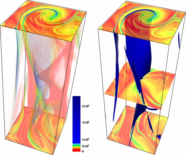
Figure 1. Two renderings of the 3D electric current density at t ∼ 30τA, when the simulation has attained a statistically steady state. Left: 3D translucent shading of the current density. Right: iso-surfaces of electric current density at a near-peak value. In both plots color contours of the current density are shown in selected cross sectional 2D planes. The legend indicates corresponding numerical values. Only 1/16 of the simulation box (0.25 × 0.25 × 10) is shown.
Download figure:
Standard image High-resolution imageIn Figure 2 we plot the PDF of the out-of-plane current density j, normalized by its rms value jrms. In this run, jrms = 1572. Recall that in RMHD the electric current density has only a z-component. Note the strongly non-Gaussian tails.
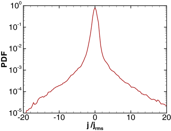
Figure 2. PDF of the current density j, normalized by its rms value (jrms = 1572).
Download figure:
Standard image High-resolution imageConditional statistics are useful to describe the extent to which the strong currents and regions of strong dissipation are space-filling. Thus let us define a cumulative density function (CDF) for the physical variable f(x, y, z) on a discrete sampling of real space points (x, y, z) as  , where ∑' includes only points where the current density is larger than a threshold value
  . Figure 3 displays the cumulative density function for the volume V and the (resistive) dissipation = ηj2. The meaning of the former quantity,
  , is the fraction of the volume for which the absolute value of j is larger than the chosen
  . The latter quantity
  is equivalent (for scalar resistivity, as employed here) to the percentage of total resistive dissipation occurring in regions with current density greater than the specified threshold
  . For example, one can infer from Figure 3 that regions with |j| > 6jrms occupy only about 0.4% of the total volume but contribute more than 50% to the total resistive dissipation. To illustrate this in a complementary way, we show in the bottom panel of the same figure the percentage of total resistive dissipation due to regions where the current exceeds
  as a function of the percentage of the volume occupied by the regions where the current exceeds the same threshold
  . One can observe that the strongest currents occupying only 0.1% of the volume contribute over 30% to the total resistive dissipation. Similarly, the top currents occupying 1% of the volume contribute about 65% to the total resistive dissipation. The dissipation in this snapshot of RMHD turbulence is therefore highly intermittent. Furthermore, from Figure 1 there is the suggestion that this dissipation is occurring in sheet-like structures that are extended in the direction parallel to the imposed mean magnetic field.
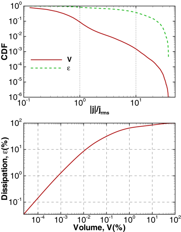
Figure 3. Top: cumulative density functions (CDF) of the volume V and the resistive dissipation = ηj2, conditioned on exceeding the normalized current density threshold |j|/jrms. Bottom: the percentage of total resistive energy dissipation in regions exceeding a current density threshold, as a function of the fractional volume (in percent) occupied by regions exceeding that current density threshold.
Download figure:
Standard image High-resolution image4. CURRENT SHEETS AND DISSIPATION
How do we define current sheets? This seemingly simple question involves several practical and subtle issues that may vary in different applications. For example, in observations from interplanetary spacecraft, current sheets are associated with tangential discontinuities, and one may wish to distinguish these from other idealized classifications of classical discontinuities. Various techniques have been employed for this purpose (Burlaga & Ness 1968; Tsurutani & Smith 1979; Neugebauer 2006). The related issue of non-Gaussian fluctuations in intermittent turbulence has motivated development of methods such as PVI (Veltri 1999; Bruno et al. 2001; Greco et al. 2008, 2009), which has a different emphasis, although it still captures both rotational and tangential discontinuities (Wang et al. 2013). More elaborate methods have also been devised to identify the hierarchy of weaker discontinuities and current structures that are expected in turbulence (Vasquez et al. 2007). For yet other methods, the angular jump of the magnetic field (rotation angle) across the current sheet is the focus (Li et al. 2011), and this approach is particularly valuable in related techniques for the identification of reconnection sites (Gosling et al. 2005). In simulations one has the advantage that the turbulent fields are known everywhere on the grid, so one can use more direct methods while also comparing the events identified with those emerging from use of the other more observationally oriented approaches (Servidio et al. 2010, 2011). Here we will adopt a simple approach in which a threshold in current density is used to find strong currents in the simulation domain. For the weakly 3D RMHD case at hand, as well as 2D cases, this approach, as we see here, identifies mainly sheet-like structures. However, in fully 3D turbulence, and especially less anisotropic 3D turbulence (Clyne et al. 2007), current structures may be more convoluted and spatially complex. In such cases a threshold based method may select a much broader class of strong current structures.
Here the specific threshold algorithm we apply for identifying structures in a high-resolution RMHD simulation will focus on finding structures in planes orthogonal to the mean field. Referring to Figure 1 one readily sees that the structures we select are predominantly cross sections of sheet-like or filamentary structures.
The algorithm begins with an interpolation of the data onto a higher resolution grid using a zero-padding technique in Fourier space which does not introduce any artificial correlation (interpolation error). (For details of the technique, see Servidio et al. 2010). Specifically, for the simulation reported on herein, each 2D plane is interpolated from its 4096 × 4096 simulation grid to an 8192 × 8192 analysis grid. This step is important for attaining the desired accuracy of our results, such as identifying the correct number of X-points and their accurate locations, as well as the statistics of current sheets including their volume, length, and width.
To locate the current sheets in a given 2D snapshot, we first scan through the data to locate all points with current density |j| above a specified threshold Jthr. In our calculation we employ Jthr ≈ 6jrms since it is empirically found to identify all the strong sheet-like current structures. We can then find both the location and the value of the maximum of |j| in each identified current sheet. A sheet is then defined as a contiguous set of points above the threshold.
Figure 4 provides an example, displaying contours of j for the midplane in the z-direction, and, in the lower panel, the identified strong current sheets. As noted above, although these strong current sheets only occupy about 0.4% of the total area, their contribution to the energy dissipation exceeds 50%.
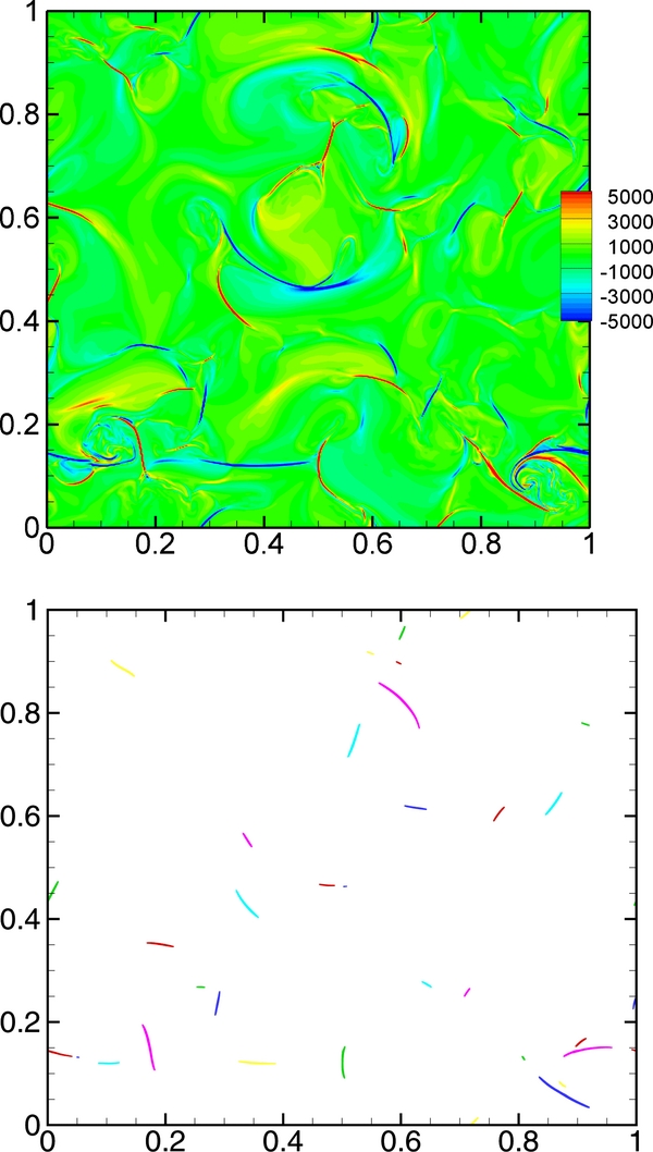
Figure 4. Top: color contour of current density field; bottom: identified strong current sheets, where |j| > 6jrms.
Download figure:
Standard image High-resolution image5. STATISTICS OF CURRENT SHEETS
We now wish to study statistical properties of the current sheets identified in the 2D (relative to  ) cross-sections of the simulation, focusing on in-plane length scales and the associated resistive dissipation rates. Recall that for RMHD models the electric current density is strictly in the parallel direction, and therefore the dissipation—controlled by
  —depends only on the two perpendicular (i.e., in-plane) coordinates. For this reason we describe here the statistical distributions of energy dissipation cs, length ℓ, and width δ, where cs is the average magnetic energy dissipated by individual current sheets per unit time, and current sheet length ℓ and width δ are measured perpendicular to the mean field. See Zhdankin et al. (2013) for discussion of the distribution of the parallel extent of the current sheets (which by definition is much larger than the perpendicular scales for RMHD). Most of our discussion will concern resistive dissipation in current sheets, although in a later section we will also remark on the statistical association of viscous and resistive contributions to dissipation.
The aspect ratio of the current sheets is of special importance in MHD models due to its connection to the theory of quasi-steady magnetic reconnection (Parker 1957). It has also been noted that current sheets and reconnection play an important role in turbulence (Matthaeus & Montgomery 1980; Matthaeus & Velli 2011); therefore, the size and aspect ratio of the current sheets that are produced by turbulence represent a key dynamical feature that controls nonlinear evolution, as has been shown recently in some detail for 2D MHD turbulence (Servidio et al. 2009, 2010). The present results are of relevance to the problem of dissipation and reconnection in the weakly 3D RMHD case.
To begin our analysis, we identified current sheets in 21 selected planes of the simulation, employing a threshold method as described above. Having selected all points within a given current sheet, the length ℓ is defined as the greatest distance between any two points in that sheet. The width δ is then the area of the current sheet divided by the length. (This is essentially identical to one of the two methods described by Zhdankin et al. 2013.)
Figure 5 illustrates a result from this method of analysis, in the form of a scatter plot of log (ℓ) versus log (δ) of the identified current sheets. For comparison, we also plot a dashed line with a slope of 0.5. Zhdankin et al. (2013) found this to be the best fit to a linear regression for these quantities.
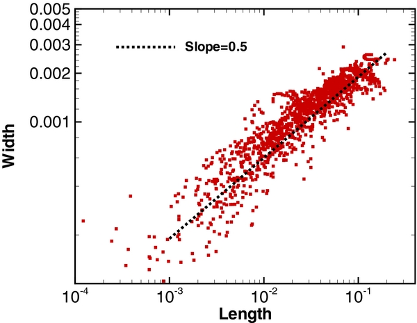
Figure 5. Scatter plot of the length vs. width of the strong current sheets. A reference line with slope 1/2 indicates scaling suggested by Zhdankin et al. (2013).
Download figure:
Standard image High-resolution imageAn interesting finding due to Servidio et al. (2010) is that in 2D turbulence, the distribution of in-plane lengths and widths of current sheets is related to the fundamental length scales associated with the turbulence cascade. A similar finding emerges here for RMHD: Figure 6 shows the PDFs of the computed lengths ℓ (in green, right side) and widths δ (in red, left side) of the identified current sheets. Also shown are the Kolmogorov dissipation scale (red dashed line, left), Taylor micro-scale (green dashed line), and correlation scale (black dashed line, right). It is readily seen that the current sheets have broadly distributed lengths ℓ, typically of the order of the Taylor microscale, but extending from the correlation scale to much smaller scales. The widths are more tightly distributed and are of the order of the Kolmogorov scale. Note that this distribution differs in a subtle way from that seen in 2D by Servidio et al. (2010). However, this may be expected in an RMHD model of coronal flux tubes (Dmitruk et al. 2003; Rappazzo et al. 2007) in which the Alfvén crossing time and line-tying are influential factors. Recently, decaying turbulence simulations of a similar setup have shown that at the peak of dissipation, the Taylor microscale is larger and total dissipation smaller for the line-tied case, when compared to the periodic case (see Figure 3 of Rappazzo & Parker 2013). Moreover, these two differences become increasingly pronounced for larger values of B0/b. Note that when there is line-tying, larger B0/b leads to stronger axial field-line tension. Indeed, for sufficiently strong values of the guide field, dissipation can be inhibited entirely. Given the strong influence of the line-tying boundary conditions on dissipation, it is therefore crucial to study the characteristics of the dissipative structures in the boundary-forced case and compare to the 2D case as done here. We note that for the relatively steep inertial range energy spectra associated with this variety of turbulence, the Taylor scale is much closer to the correlation scale (or energy-containing scale) than it is for shallower spectra. We review the relevant physics in the Appendix.
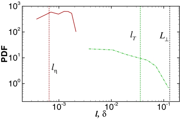
Figure 6. PDFs of the length ℓ (green dash-dotted line) and width δ (red solid line) of the identified current sheets. Also shown are the Kolmogorov dissipation scale, ℓη (red dashed vertical line at left), Taylor micro-scale, ℓT (green dashed vertical line at center) and correlation scale, L⊥ (black dashed vertical line at right). The widths are distributed about the Kolmogorov scale, while the lengths are broadly distributed about the Taylor scale, ranging from correlation scale to much smaller scales.
Download figure:
Standard image High-resolution imageThe average dissipation rate cs computed within a current sheet (cross-section) as a function of the area of the current sheet is shown in Figure 7. (Note that as defined, cs × area = the total Ohmic dissipation in the current sheet cross-section.) Also shown is the average Ohmic dissipation rate computed over the entire simulation domain. It is clear that current sheets in general have an average dissipation rate much higher than the global average dissipation rate, as expected. It is also readily seen that the current sheets that are of smaller area have an average dissipation rate that is roughly independent of size. The larger current sheets however have larger average dissipation rates. This appears to be compatible with the finding of Servidio et al. (2010) that the fastest reconnection rates are found among the population of 2D current sheets that have the largest lengths ℓ. A reasonable interpretation is that the formation of the most intense current sheets occurs as a consequence of the collision between larger magnetic islands (or flux tubes) which produces a larger region of interaction. Sweet (1958) described this phenomenon as "analogous to the flattening of a motor tyre when loaded." This also causes closer encounters and therefore smaller thickness δ and larger current density.

Figure 7. Scatter plot of the average dissipation of the current sheets cs vs. the cross-sectional area of the current sheets. The global average dissipation of the whole field, 〈〉, is shown as the black dashed line. A level line is also shown corresponding well to the behavior of the average dissipation for small area current sheets. The blue solid line indicates a power law index of 0.1, as found by Zhdankin et al. (2013) using a somewhat different method of current sheet identification.
Download figure:
Standard image High-resolution imageAnother result is shown in Figure 8, which displays the locations of strong current sheets and strong vortices. It is apparent that enhancements of both vorticity and current are roughly sheet-like, and that they are also nearly co-located. This is consistent with the known association of quadrupolar vorticity distributions with active, reconnecting current sheets in 2D MHD (Matthaeus 1982). Note that in this perspective the vorticity is generated by the circulation of the Lorentz force near the current sheet. Vorticity generated in this way is expected to be located very near current sheets—more precisely, near positions in which the local magnetic field overlaps regions of strong gradients of the current density. A close-up illustration of the region near one selected current sheet is shown as an inset within Figure 8. The signed vorticity is plotted, confirming that the distribution is indeed quadrupolar, centered around the current sheet. The preference for this spatial relationship between current and vorticity is revealed quantitatively by analysis of the two-point correlation function of the out-of-plane components of vorticity and current density. The interpretation of these correlations provides a consistent picture. Shown in Figure 9 is the "Type I" correlation  of the signed vorticity and current density, and the "Type II" correlation
  for the absolute values of the same quantities. Both correlations are normalized by the product of the respective rms values of the fields used in the correlations.
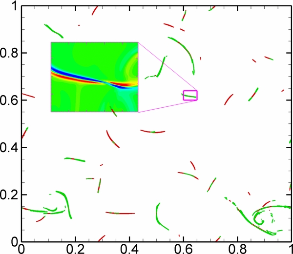
Figure 8. Scatter plot of strong current sheets (in red) and vortices (in green), demonstrating that these regions are often nearly co-located. The inset shows a magnification of one such region, showing the signed vorticity. It is clear that this vorticity enhancement, like most of the others, has a quadrupolar character.
Download figure:
Standard image High-resolution image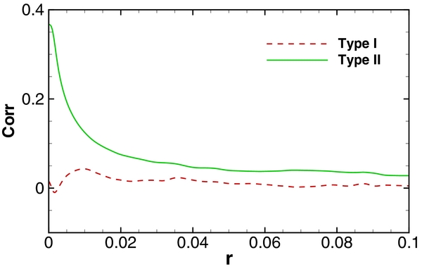
Figure 9. Correlation of the out-of-plane components of vorticity and current density. Type I:  for the signed vorticity and current density; Type II:
  for absolute values of the same quantities. Both quantities are normalized by the rms values of vorticity and current density.
Download figure:
Standard image High-resolution imageFrom Figure 9 it is readily seen that the signed correlation hovers near zero, indicating that whatever correlation exists is nearly the same for positive and negative vorticity. Meanwhile the absolute value correlation remains nonzero out to a distance of the order of r = 0.01 to 0.02.
6. RECONNECTION AND CRITICAL POINTS IN REDUCED MHD
The highly localized sheet-like current structures described above are immediate causes of intermittency and enhanced dissipation in driven RMHD, consistent with analogous effects in two dimensions. Indeed these properties are central in the turbulence interpretation of the statistics of nanoflares (Einaudi & Velli 1999; Rappazzo et al. 2013). The status of reconnection association with these current sheets is less certain. Indeed, although RMHD has some 3D effects (and eliminates the extra constraints present in the strictly 2D case), it is nonetheless possible to have strong current sheets that have weak reconnection rates. This is a direct consequence of the fact that in the RMHD model the magnetic potential does not in general define magnetic surfaces (Servidio et al. 2014). One implication is that (component) magnetic X-points have a far weaker association with current sheets (Zhdankin et al. 2013) than is found in the standard 2D paradigms of reconnection (Sweet 1958; Parker 1957; Petschek 1964). To quantify the features of reconnection in the present RMHD model, we proceed to directly analyze the properties of the computed critical points.
Using the method developed in Servidio et al. (2009, 2010, 2011), we can identify potential reconnection sites in the RMHD simulation, which are the X-points of the in-plane magnetic field, i.e., saddle points of the magnetic potential in the selected x–y plane. Current sheets may or may not coincide with magnetic X-points (Rappazzo & Velli 2011; Zhdankin et al. 2013). An example from the simulation is shown in Figure 10, which displays in-plane magnetic field lines along with contours of j. Identified reconnection sites (X-points) are shown with the symbol "X."
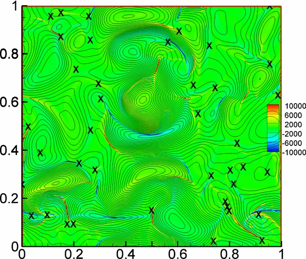
Figure 10. Color contour of current density with in-plane magnetic field lines. Identified magnetic X-points, which are potential reconnection sites, are shown with symbol "X." It is evident that many X-points are not located at strong current sheets, as noted by Zhdankin et al. (2013).
Download figure:
Standard image High-resolution imageHaving obtained the positions of the X-points, we may then compute the reconnection rates as (minus) the electric field at the X-point, or equivalently the rate of change of the magnetic flux in the strong field regions adjoining the X-point:
Here EX is an abbreviation for the electric field measured at the (X-point) saddle point. Clearly, the reconnection rate at the X-point is EX = −ηJX, where JX is the current density at the X-point. The PDF for |EX|, in Alfvén units, is shown in Figure 11. This indicates that low reconnection rates are the most likely. However, there are a substantial fraction of cases in which |EX| > 0.1, which may nominally be viewed as a "fast" rate of reconnection when referred to the global Alfvén speed. The average value of reconnection rate in this distribution is 0.039 in the Alfvén units we employ.

Figure 11. PDFs of three different samples of the electric field. Solid red line: PDF of the reconnection rate at X-points, |EX| in Alfvén units. Note that the reconnection rate EX = −ηJX, where JX is the current density at the X-points. Also shown are the PDFs of  and η|j|, from all grid points with 3 < z < 7. The large values of electric fields at X-points that produce large reconnection rates are more probable than the same values in the Ohmic electric field accumulated from the entire simulation. However, similarly large values of ambient induced electric field are more probable.
Download figure:
Standard image High-resolution imageTo study the relation of current sheets and X-points, we ask whether each X-point lies within an identified current sheet, and then, how far are the outlying X-points from the nearest current sheets. To answer these questions, we computed the shortest distance between an X-point and any point in a nearby current sheet. We show the PDF of this distance from X-points to the closest current sheet, normalized by the Kolmogorov dissipation scale ℓη, in the top panel of Figure 12. An X-point is considered to lie inside a current sheet when the distance is smaller than one grid length, Δx = 1/4096 ≈ 2.5 × 10⁻⁴, which is indicated by the vertical dashed line in Figure 12. In this simulation, we do find some X-points lying inside current sheets, although the exact number depends on the particular threshold value Jthr employed in defining the current sheets.

Figure 12. Top: PDF of the distance (r) from X-points to the closest current sheet (region with |j| ≳ 6jrms), normalized by the Kolmogorov dissipation scale ℓη. Bottom: conditional average of electric field at the X-points, conditioned on the distance from the X-point to the closest current sheet. Grid length, Δx, is indicated in both panels by vertical dashed lines.
Download figure:
Standard image High-resolution imageHaving established that both the reconnection rates and the distances of X-points from current sheets are widely distributed, the next question of interest concerns the possible association of the reconnection rates with the distance between X-points and current sheets. In the lower panel of Figure 12 we plot the conditional average of reconnection rates at the X-points EX, conditioned on the distance of the X-point to the closest current sheet. Again, EX is in Alfvén units. A remarkable feature of these distributions is that they are very broad, with distances between X-points and the nearest current sheet ranging from less than a Kolmogorov scale (meaning the X-point is effectively within the current sheet), to more than 100 Kolmogorov scales. It is interesting, and physically appealing, to recognize that the reconnection rates are on average much higher when the X-points and current sheets have greater propinquity, while distant X-points have systematically weaker reconnection activity. In fact beyond two or three Kolmogorov scales the reconnection rates are already very weak, and fall off only very slowly for greater distances. For 3D reconnection this effect may help explain why reconnection in solar contexts is not always very fast, so that energy may be built up and stored for a significant period of time, prior to release by rapid reconnection.
Having identified all the X-points in 2D planes, it is useful to illustrate the positions of the X-points in the 3D domain, which then permits a visual interpretation of the extent of component X-lines in the direction of the strong mean magnetic field. This is shown in Figure 13. This rendering clearly suggests the extent of X-lines in the 3D geometry, even though the tracing was not carried out in three dimensions. Close inspection suggests that some X-lines bifurcate, and in other instances, X-lines merge. The color of the points represents the value of current density at the X-points, which reveals that a given X-line may coincide with a strong current sheet for only part of its parallel extent. The red color represents X-points with current density larger than Jthr = 9240, which indicates that those X-points are lying inside what we have defined as a strong current sheet. It is clear that some X-lines have a moderately strong (but subthreshold) current density along their entire extent.

Figure 13. 3D picture of X-lines in the simulation box. X-points are color-coded according to the value of |j| there. Red points represent X-points with current density larger than Jthr = 9240 ≈ 6jrms, which indicates that those X-points are lying inside the current sheets.
Download figure:
Standard image High-resolution imageFinally, as noted above, the magnetic potential does not define field lines in RMHD, so it is not expected that the apparent trajectories of the X-points (Figure 13) in 3D space would coincide with field lines. In addition, the current is not constant along field lines, so the spatial extension of the strong current sheets is still another independent feature. Figure 14 demonstrates the independence of current sheets and X-lines by illustrating one selected case from the simulation. The independence of these features represents a complexity of the 3D problem that is evidently already appearing in the weakly 3D RMHD model.

Figure 14. Zoom-in of the simulation box, showing the iso-surfaces of the current density field and a line of identified X-points in black dots. Color bar is for the current density.
Download figure:
Standard image High-resolution image7. DISCUSSION AND CONCLUSIONS
The present analysis of current sheets, vortex structures, and reconnection rates in RMHD, along with the recent complementary study by Zhdankin et al. (2013), serves to extend analysis of the statistics of 2D MHD reconnection (Servidio et al. 2009, 2010) and current sheets (Greco et al. 2008, 2009; Li et al. 2011) to the weakly 3D RMHD case. It is clear that there is much in common between the weakly 3D case and the 2D case. Both of these have been characterized here for the familiar special case that includes only polarizations that are transverse to a mean magnetic field. This case, known as the "Alfvén mode," involves only one potential function, the toroidal one (see, e.g., Oughton et al. 1997). The fully 3D case requires two scalar potentials to describe a general solenoidal magnetic field, and may be expected to admit more complex correlations (Oughton et al. 1997), more complex topologies (e.g., Priest & Pontin 2009), and more complex coherent structures (e.g., Mininni et al. 2008). Nevertheless the RMHD case remains of interest, mainly because of its relevance to low plasma beta, nearly incompressible, strong guide field applications such as coronal loops and coronal hole flux tubes and some laboratory and astrophysical plasmas (e.g., Strauss 1976; Zank & Matthaeus 1992, 1993; Einaudi et al. 1996; Hendrix & van Hoven 1996).
The present analyses have shown that in a model relevant to coronal loops, many reconnection sites are established, consistent with the nanoflare scenario (Parker 1972; Einaudi & Velli 1999; Dmitruk et al. 1998; Rappazzo et al. 2013). The sizes of the current sheets are widely distributed, with the perpendicular lengths and widths related to the turbulence characteristic scales, as they were found to be in the 2D case (Servidio et al. 2010). The reconnection rates are also similarly found in a broad distribution (for the 2D case, see Servidio et al. 2010) with some fast reconnection rates >1/10 (Alfvén units) found. However the average reconnection rate is somewhat reduced by the interesting finding (see Zhdankin et al. 2013) that the component X-points (which form the center of reconnection activity) and the current sheets are often displaced spatially from one another. This is evidently a 3D effect. It can occur (in a mathematical sense) in RMHD because the magnetic potential is not constant along field lines or flux surfaces (Servidio et al. 2014), whereas it is constant in 2D. The physical effect that drives the separation of X-points and current sheets in RMHD is evidently the long wavelength wave propagation that occurs here but not in 2D. Only when the current sheets and X-points do coincide does one find the strongest resistive electric fields at X-points and therefore the strongest reconnection rates. This effect appears to be a fundamental feature that impacts the intermittent nature of reconnection and heating in the turbulence picture of nanoflares (Dmitruk et al. 1998; Einaudi et al. 1996).
The strong current sheets associated with reconnection are also found here to be accompanied by strong enhancements of vorticity. This is consistent with the quadrupolar picture of vorticity generation near current sheets (Matthaeus 1982). These vortices are the characteristic small-scale structures responsible for intermittency in the velocity field, just as current sheets are the coherent structures related to intermittency of the magnetic field. This picture, familiar in 2D (Matthaeus & Montgomery 1980; Biskamp 1986; Carbone et al. 1990; Veltri 1999), is evidently found also in the weakly 3D case. Again, as with the current structures, the fully 3D case is expected to be more complex (Mininni et al. 2008).
Both vorticity and current enhancements are sites of enhanced dissipation in RMHD and are likely also sites of dissipation in the kinetic plasma regime (not studied here). The results also show that the current and vorticity enhancements are widely distributed in size. However it is also found that the average Ohmic heating rate in current sheets is relatively insensitive to the size of the current structure for small structures. The average heating rate increases with increasing size for the larger current sheets. This appears to be associated with the driving of current enhancements and reconnection due to collisions between flux tubes, as it is in the 2D case. This feature stands in contrast to the expectations of reconnection when viewed as a spontaneous rather than a driven process. For example, in the simplest interpretation of Sweet–Parker theory, the reconnection rate goes as  where Rm = cAL⊥/η, and longer current sheets would have slower reconnection rates. However, as we have seen, this is not the case in turbulence.
This research is supported in part by the NSF Solar Terrestrial Program Grant AGS-1063439 and SHINE grant AGS-1156094, NASA Heliophysics Grand Challenges program (NNX14AI63G), Delaware NASA/EPSCoR Program NNX13AB30A, the MMS Theory and modeling project, the Solar Probe Plus ISIS project. Part of the computational resources were provided by the NASA High-End Computing (HEC) Program through the NASA Advanced Supercomputing (NAS) Division at Ames Research Center. S.S. acknowledges funding from the European Communitys Seventh Framework Programme (FP7/2007-2013) under grant agreement no. 269297/"TURBOPLASMAS" and POR Calabria FSE 2007/2013. A.F.R. is supported in part by a subcontract with JPL.
APPENDIX: SPECTRUM SLOPE AND RMHD LENGTH SCALES IN CORONAL LOOPS
When the omnidirectional energy spectrum  is of the Kolmogorov type—here meaning it has a power-law inertial range—one expects that the correlation scale L⊥, Taylor scale ℓT, and Kolmogorov dissipation scale ℓη are related as ℓT = L⊥/R1/2 and ℓη = L⊥/R3/4, where R is the large-scale Reynolds number R = ZL⊥/η with turbulence amplitude Z and dissipation coefficient η. Here the correlation scale is
  with R the standard spatial correlation function, and the upper limit w is taken to be halfway across the simulation box. The Taylor scale is obtained from
  with the brackets denoting a volume average. The Kolmogorov scale is estimated from the standard formula ℓη = (/η3)1/4 with the rate of Ohmic dissipation.
In the strongly turbulent regime, the Taylor scale is much closer to the Kolmogorov scale in that L⊥/ℓT ≫ ℓT/ℓη when R ≫ 1. However this conclusion depends sensitively on the energy spectrum  having a power-law index α ≈ 5/3. In fact when the index is steeper than α = 2, the Taylor scale becomes more sensitive to the correlation scale and less sensitive to the Kolmogorov scale.
Coronal loop models have the interesting property that the correlations that drive the energy cascade may be limited by local nonlinear distortions (as in Kolmogorov theory) but also other effects, such as wave propagation through the loop (Dmitruk et al. 2003; Zhou et al. 2004; Rappazzo et al. 2007). In a loop with a strong axial magnetic field, the lifetime of the higher order correlations may depend essentially only on the Alfvén speed and parallel wavenumber while the nonlinear effects depend only on perpendicular wavenumber. In such cases the energy spectra can behave as k−2 or even k−3. In that limit the Taylor scale may be closer to the correlation scale, with L⊥/ℓT < ℓT/ℓη. This at least partially explains the difference in scaling of current sheet in-plane lengths and widths (ℓ and δ) seen in Figure 6 above for the coronal loop RMHD case shown in this paper and the analogous 2D results evident in Figure 19 of Servidio et al. (2010). This interpretation is supported by the steepness of the energy spectrum in the present simulation, illustrated in Figure 15. For this simulation the in-plane magnetic spectrum is found to have a slope close to −8/3 in the inertial range.

Figure 15. Spectrum of the in-plane magnetic field.
Download figure:
Standard image High-resolution image