


ABSTRACT
In astrophysical plasmas, magnetic field lines often guide the motions of thermal and non-thermal particles. The field line random walk (FLRW) is typically considered to depend on the Kubo number R = (b/B0)(ℓ∥/ℓ⊥) for rms magnetic fluctuation b, large-scale mean field B0, and parallel and perpendicular coherence scales ℓ∥ and ℓ⊥, respectively. Here we examine the FLRW when R → ∞ by taking B0 → 0 for finite bz (fluctuation component along B0), which differs from the well-studied route with bz = 0 or bz ≪ B0 as the turbulence becomes quasi-two-dimensional (quasi-2D). Fluctuations with B0 = 0 are typically isotropic, which serves as a reasonable model of interstellar turbulence. We use a non-perturbative analytic framework based on Corrsin's hypothesis to determine closed-form solutions for the asymptotic field line diffusion coefficient for three versions of the theory, which are directly related to the k−1 or k−2 moment of the power spectrum. We test these theories by performing computer simulations of the FLRW, obtaining the ratio of diffusion coefficients for two different parameterizations of a field line. Comparing this with theoretical ratios, the random ballistic decorrelation version of the theory agrees well with the simulations. All results exhibit an analog to Bohm diffusion. In the quasi-2D limit, previous works have shown that Corrsin-based theories deviate substantially from simulation results, but here we find that as B0 → 0, they remain in reasonable agreement. We conclude that their applicability is limited not by large R, but rather by quasi-two-dimensionality.
Export citation and abstract BibTeX RIS
1. INTRODUCTION
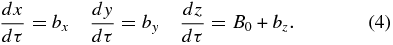
In many astrophysical plasmas, magnetic field lines play a key role in organizing the transport of both the bulk plasma and energetic particles. In many cases, the magnetic field is highly turbulent, which leads to a random walk of magnetic field lines and diffusion of particles distributions both along and perpendicular to the mean field (Jokipii 1966; Jokipii & Parker 1968). These processes underlie numerous astrophysical phenomena, such as the transport of solar energetic particles to Earth (Meyer et al. 1956), solar modulation of Galactic cosmic rays (Rao 1972; Moraal 1976), diffusive shock acceleration (Drury 1983), propagation of cosmic rays and diffuse gamma-ray emission in the Galaxy (Ackermann et al. 2012), and possibly the "moss" emission in the solar transition region (Kittinaradorn et al. 2009).
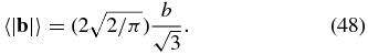
Theoretical concepts of the magnetic field line random walk (FLRW) have mostly been developed in studies that consider the rms fluctuation b to be much weaker than the large-scale field B0 (Isichenko 1991a, 1991b) or for transverse turbulence with b⊥B0, i.e., bz = 0 where  is along B0 (see Matthaeus et al. 1995; Shalchi 2009; Ruffolo & Matthaeus 2013, and references therein). In these cases, characterized by bz ≪ B0, there is a scaling relation by which the asymptotic field line diffusion coefficient depends on the dimensionless ratio (b/B0)(ℓ∥/ℓ⊥), where ℓ∥ and ℓ⊥ are length scales parallel and perpendicular to B0, respectively (Ghilea et al. 2011). For some magnetic fluctuation models, such as the 2D+slab model (Matthaeus et al. 1995), the parallel and perpendicular correlation scales are infinite, so we use the finite coherence scales of individual components for the scaling relation (Ghilea et al. 2011; Snodin et al. 2013a). When the correlation scales are well defined, ℓ∥ and ℓ⊥ can be set to the correlation scales, and the above dimensionless ratio is identified with the Kubo number, R (Kubo 1963). For R ≪ 1, or fluctuations dominated by wave vectors nearly parallel to B0, which can be described as "slab" or quasi-one-dimensional fluctuations, all accepted theories and computer simulation results agree with the quasilinear theory of Jokipii & Parker (1968), with D = (b/B0)2(λc/2) for the parallel correlation scale λc.
In contrast, for fluctuations with bz ≪ B0 and R ≫ 1, there is no general consensus on how to model the FLRW. Such fluctuations are quasi-two-dimensional (quasi-2D), dominated by wave vectors nearly perpendicular to B0. In this case, there are strong trapping effects in which some field lines are trapped in topological structures either temporarily or permanently. Such trapping is associated with conservation of the flux function (for purely 2D fluctuations) or approximate conservation of a related quantity (for quasi-2D fluctuations), leading to (x, y) trajectories that are nearly closed and periodic. Corrsin's hypothesis (Corrsin 1959), a theoretical approximation to be described later in this work, is quite accurate at low Kubo number and even up to R ∼ 10 (Snodin et al. 2013b), but becomes less accurate at higher R because it does not include the "memory" effect of trapping (Vlad et al. 1998; Ruffolo et al. 2008). Other proposed theories have been based on percolation (Gruzinov et al. 1990) or decorrelation trajectory methods (Vlad et al. 1998). None have been conclusively shown to accurately model the asymptotic diffusion coefficient D at very large R values.
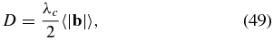
The physical reason for the change in FLRW from the quasi-linear regime (at R ≪ 1) to the quasi-2D regime (R ≫ 1) is that the former has "extrinsic" decorrelation, where the magnetic field changes (decorrelates) because the mean field carries the field line across domains of size ∼ℓ∥ and the latter has "intrinsic" decorrelation, where the field line crosses domains of size ∼ℓ⊥ due to its own random walk. In theories based on Corrsin's hypothesis, for situations with bz ≪ B0, this distinction results in D ∼ (b/B0)2ℓ∥ for the quasilinear regime with extrinsic decorrelation and D ∼ (b/B0)ℓ⊥, known as "Bohm diffusion," for the quasi-2D regime with intrinsic decorrelation (Matthaeus et al. 1995; Ruffolo et al. 2004). However, a random walk with intrinsic decorrelation can be subject to trapping effects, especially in a quasi-2D regime where the projected 2D trajectory is topologically constrained to a nearly closed path (Ruffolo et al. 2008). This leads to the failure of Corrsin's hypothesis in the quasi-2D limit and poses a continuing challenge to other theories as well.
In the present work, we examine a different route to the limit of R = (b/B0)(ℓ∥/ℓ⊥) → ∞: instead of taking ℓ∥/ℓ⊥ → ∞ for finite b/B0 (the quasi-2D limit), we examine the limit of B0 → 0 for finite ℓ∥/ℓ⊥. Physically, when there is little or no large-scale field, there is no preferred direction and it is natural to consider the turbulence to be isotropic in three-dimensional (3D) wave number space. Isotropic 3D turbulence with no mean field provides a reasonable description of magnetic fluctuations in the interstellar medium of our Galaxy, which has a well-developed turbulent cascade (Armstrong et al. 1995) and a fluctuation field of the same order of magnitude as a Galactic field that itself reverses on larger scales (Minter & Spangler 1996) and might be considered to have an average value near zero. To our knowledge, the FLRW has not previously been examined for this case. For basic understanding of FLRW theory, B0 = 0 is a case of infinite Kubo number with purely intrinsic decorrelation that is not quasi-2D. Without an analog to a conserved flux function, this case of isotropic 3D turbulence with zero mean field may not exhibit the strong topological trapping of the quasi-2D limit, although three-dimensionality introduces new possibilities for trapping, e.g., in closed magnetic structures. Here we consider how to parameterize the FLRW in the absence of a large-scale field and examine how the existing theoretical concepts for bz ≪ B0 should scale for the case of low B0. We then develop analytic theories for asymptotic field line diffusion coefficients based on Corrsin's hypothesis. We also perform direct computer simulations of isotropic turbulence with no mean field and trace individual field lines from random initial locations. An example of one such field line is shown in Figure 1. From an ensemble of such field lines, we computationally determine the diffusion coefficient and compare with results from the analytic theories.

Figure 1. Example of a magnetic field line in a realization of isotropic turbulence with a zero mean field. We use statistics from an ensemble of such random walks to determine the field line diffusion coefficient and compare with theoretical expectations.
Download figure:
Standard image High-resolution image2. DESCRIPTIONS OF FIELD LINE DIFFUSION
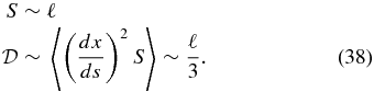
While this study will focus on isotropic turbulence with zero mean field, to relate our results to the previous literature, it is instructive to first examine a more general magnetic field given by 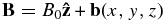 . If the magnetic fluctuation b has a finite correlation length, then the FLRW is expected to exhibit diffusive behavior. We now have a choice of how to parameterize the diffusive process.
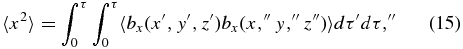
In the cases of transverse turbulence, in which the magnetic fluctuations are always perpendicular to the mean field, it is natural to describe the perpendicular (x, y) motion of a field line as a function of the coordinate along the mean field, z. Such a description has also been used for 3D turbulence in the case that bz ≪ B0 (e.g., Jokipii & Parker 1968). Then the field line trajectory is described by
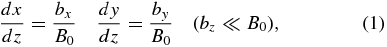
where, for convenience, we set x = y = 0 at z = 0. In an astrophysical plasma, there is typically a finite coherence scale and the distribution of the displacement (x, y) exhibits asymptotic diffusion at large z. In, say, the x direction, the asymptotic diffusion coefficient is limz → ∞〈x2〉/(2z) and a running diffusion coefficient can be defined as (1/2)d〈x2〉/dz.
However, the present study focuses on the case of isotropic 3D turbulence with no mean field, in which case we should avoid special treatment of any coordinate. Indeed, with turbulent fluctuations that are both positive and negative in all directions, the field line trajectory moves back and forth in each direction, so for a given z there may be multiple points in the x–y plane on the same field line. Thus functions such as x(z) and y(z) may not be single-valued, and the z coordinate (or any other Cartesian coordinate) cannot be used to parameterize the field line. In this section, we consider parameterizations that can be used for any value of B0, even B0 = 0.
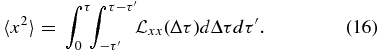
One parameterization describes the motion in each coordinate as a function of the arclength s along the field line, with
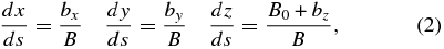
where  . This can also be written as
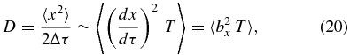
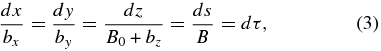
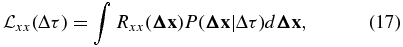
so that the same field line can also be described in terms of a parameter τ defined by dτ = ds/B:
We find this parameterization to be more convenient for analytic calculations and more conducive to theoretical insight. In terms of s, we can define diffusion coefficients by
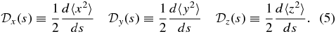
In terms of τ, we define
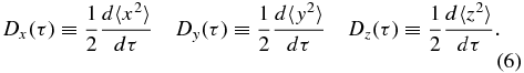
We note that the relationship between τ and s depends on the local magnetic field along the field line trajectory. As an aside, note that Equations (4) describe streamlines in a fluid if the magnetic field B is replaced by a velocity field v and τ is replaced by time.
Previous work on the diffusive FLRW has identified three types of diffusion: quasilinear, Bohm, and percolation/trapping. First, consider the case where bz is negligible and we use dimensionless variables x' = x/ℓ⊥, y' = y/ℓ⊥, and z' = z/ℓ∥. Then Equations (1) become
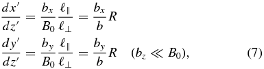
where in this context we may define 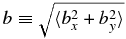 . Most seminal work on the FLRW considered this case (e.g., Jokipii & Parker 1968; Kadomtsev & Pogutse 1979; Isichenko 1991a, 1991b; Matthaeus et al. 1995). If the fluctuations are axisymmetric, so that bx and by are statistically identical, or if they remain comparable and scale with b, then the dimensionless diffusion coefficients depend only on R. For nonaxisymmetric turbulence, dimensionless diffusion coefficients depend on both R and the rms value of bx/b (e.g., Zimbardo et al. 2000; Ruffolo et al. 2006; Weinhorst et al. 2008). For the Kubo number dependence, we may have
  , including the cases
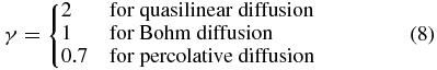
(Jokipii & Parker 1968; Salu & Montgomery 1977; Isichenko 1991b). All authors agree that quasilinear diffusion applies at R ≲ 1 (except that Ruffolo et al. (2006) expect Bohm diffusion for cases of extreme nonaxisymmetry) and the other types of diffusion have been proposed for R ≳ 1, along with some theories predicting that γ depends on the magnetic fluctuation model and its Eulerian correlation function (e.g., Vlad et al. 1998; Vlad & Spineau 2014). In any case, for the values in Equation (8), the dimensional asymptotic diffusion coefficients for the case of negligible bz are
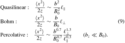
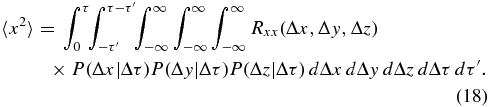
Now consider the generalization of those prior results to the case where bz is not small. We can no longer use z to parameterize the FLRW. Here we consider parameterization in terms of τ and consider diffusion coefficients in terms of τ as in Equation (6). Using τ' = τB0/ℓ∥, we can convert Equations (4) to dimensionless form:
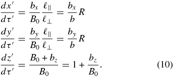
When bz is negligible, these equations imply dz' = dτ' and exactly correspond to Equations (7). Thus we generalize the asymptotic power-law behavior at low bz, 〈x'2〉/(2z') ∼ Rγ, to general bz by using τ' = z', which implies τ = z/B0. Then Equations (9) correspond to diffusion coefficients as
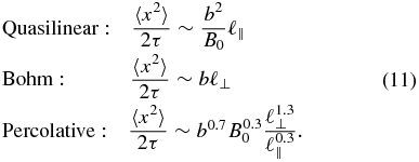
In the present work, we will use analytic and computational techniques to determine which of these forms for asymptotic diffusion coefficients in terms of the parameter τ is applicable in the limit B0 → 0, which represents an alternative route to R → ∞. In this limit, a quasilinear coefficient would diverge, a Bohm coefficient would remain finite, and a percolative coefficient would tend to zero. In other words, the FLRW would be superdiffusive, diffusive, or subdiffusive, respectively.
Finally, to examine 〈x2〉/(2s), in terms of the more common parameterization s, we note that ds = Bdτ and consider the limiting cases of B0 ≪ b and B0 ≫ b. For these, we use ds = bdτ and ds = B0dτ, respectively, to obtain the following asymptotic behavior:
Contrasting Equations (11) and (12), for the s parameterization we should not expect a single power-law scaling of the diffusion coefficients over both high and low b/B0. Indeed, if we attempt to apply distinct scaling in the parallel direction (by ℓ∥) and perpendicular direction (by ℓ⊥), then s itself, which combines parallel and perpendicular motion by 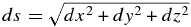 , does not have a simple scaling. Furthermore, theoretical calculation of these diffusion coefficients by integrating Equations (2) would be difficult because they involve
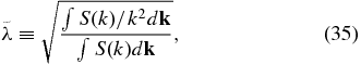
 ![$B^{-1} = [b_x^2 + b_y^2+(B_0+b_z)^2]^{-1/2}$](https://content.cld.iop.org/journals/0004-637X/798/1/59/revision1/apj504699ieqn7.gif) , which is nonlinear in the fluctuation b. In the following section, we will instead derive the field line diffusion coefficients in terms of τ.
, which is nonlinear in the fluctuation b. In the following section, we will instead derive the field line diffusion coefficients in terms of τ.
3. ANALYTIC THEORY FOR ZERO MEAN FIELD
3.1. Basic Theory
We consider the FLRW for homogeneous, isotropic turbulence with no mean magnetic field. With isotropy, we can assume the fluctuations in the x, y, and z directions to be statistically identical, and with no mean field, the diffusion coefficients in each direction are the same:

When we write D or  with no functional dependence, we are referring to the asymptotic limit at large τ or s, respectively. The following derivation is similar to that of Ruffolo et al. (2004).
For zero mean field, we use B0 = 0 in Equations (4). Then following Jokipii & Parker (1968), we express the displacement in, say, the x coordinate of a field line over τ by
The ensemble average variance is then given by
where we introduce the notation x' for x(τ'), x'' for x(τ''), etc. Setting Δτ ≡ τ'' − τ', and with the assumption of homogeneity,
We use the symbol  to denote the ensemble average Lagrangian correlation of bx at two locations along the same magnetic field line separated by Δτ.
The Lagrangian correlation function differs from a standard (Eulerian) correlation function in that the positions themselves depend on the field line trajectory. The Eulerian correlation function is the inverse Fourier transform of the power spectrum, which can often be specified based on physical considerations. It is possible to relate the Lagrangian correlation function  to the Eulerian correlation function Rxx (and thence the power spectrum) using the following approximation:
where P(Δx|Δτ) is the distribution of the displacement  of field lines after Δτ. This approximation is known as Corrsin's independence hypothesis (Corrsin 1959; Salu & Montgomery 1977; see also McComb 1990). Computer simulations have been used to verify that theories based on Corrsin's hypothesis are successful for the FLRW (Gray et al. 1996; Ghilea et al. 2011) and field line separation (Ruffolo et al. 2004) in two-component turbulence and the FLRW in reduced magnetohydrodynamic (RMHD) turbulence (Snodin et al. 2013b), except that limiting quasi-2D cases can be problematic. The limitation of Corrsin's hypothesis is that it accounts for Lagrangian trajectories in terms of the two-point Eulerian correlation, so it does not account for coherent structures or for "memory" in the random walk, which occurs for nearly 2D turbulence because the FLRW can be temporarily trapped in "islands" with closed 2D trajectories (Ruffolo et al. 2003; Chuychai et al. 2007; Seripienlert et al. 2010).
We employ Corrsin's hypothesis and use P(Δx|Δτ) = P(Δx|Δτ)P(Δy|Δτ)P(Δz|Δτ) because of the statistical independence of Δx, Δy, and Δz, which is exact for our present case of isotropic turbulence and mirror symmetry, and also for some other symmetries. Then substituting Equation (17) into Equation (16) yields
3.2. Diffusive Decorrelation
There are different versions of the theory. Here we start by using diffusive decorrelation (DD; Taylor & McNamara 1971; Salu & Montgomery 1977; Matthaeus et al. 1995). The key assumptions of DD are that the magnetic field lines spread diffusively over the decorrelation scale of the random walk and their distributions are Gaussian. Thus the displacement distributions P of the DD model are Gaussian with variances

where D is the asymptotic diffusion coefficient in terms of τ (see Equations (6) and (13)).
Before delving deeper into the mathematical derivation, let us consider a simple conceptual derivation (adapted from Ruffolo et al. 2004):
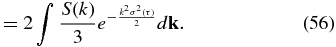
where T represents the τ scale over which bx decorrelates and thus can be considered a "mean free τ." This FLRW is entirely "intrinsic," i.e., the decorrelation depends entirely on the FLRW itself. Suppose the decorrelation occurs over a spatial scale ℓ. Then for DD, we use
where b2 ≡ 〈|b|2〉. Note that in the above, T is expressed in terms of ℓ and D, which are constant for all field line trajectories in the ensemble. We obtain a diffusion coefficient in the form of Bohm diffusion as derived in Section 2 (see Equation (11)).
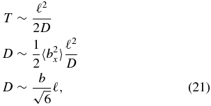
Similarly, for  , the diffusion coefficient in terms of s,
where S is a "mean free s." For DD, we use
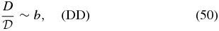
Then the ratio between the two diffusion coefficients is expected to be

the rms fluctuation, a prediction that is independent of the form of the power spectrum.
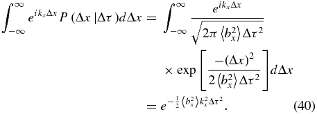
To continue the mathematical derivation of D, we make use of the power spectrum Sxx(k):
Note that for Gaussian P,
which makes use of Equation (19), and with the analogous formulae for the Δy and Δz integrals, we obtain
Note that Sxx(k) as used here follows a different Fourier transform convention than Pxx(k) as used in some of our previous work. The physical results do not depend on the convention used. Effectively, for the determination of the asymptotic diffusion coefficient at large τ, the limits of integration over Δτ in Equation (27) can be taken to be −∞ and ∞ (Jokipii & Parker 1968). In this diffusive regime, we have <x2 > =2Dτ and
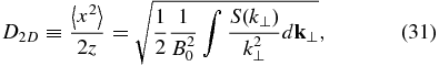
In terms of the modal energy spectral density S(k) = Sxx(k) + Syy(k) + Szz(k), which for isotropic turbulence is a function only of the wavevector magnitude k, we have
In terms of the arclength, parameterized by ds = Bdτ, we can estimate the diffusion coefficient  using Equation (24):
These diffusion coefficients are quite similar to that obtained by Matthaeus et al. (1995) for a 2D axisymmetric component of transverse turbulence with a mean field B0:
where z serves to parameterize the FLRW, k⊥ ≡ (kx, ky), and  . The only differences in these expressions are due to the different dimensionality n (n = 3 for isotropic 3D turbulence, n = 2 for 2D turbulence, which appears in the factor 1/n inside the square root), and the magnetic field component associated with the independent variable (not used for isotropic turbulence in terms of τ; b for isotropic turbulence in terms of s; and B0 for 2D turbulence in terms of z). The reason for the similar expressions is that both diffusion processes are intrinsic, involving random flights in which the magnetic fluctuation along the trajectory decorrelates stochastically due to the random motion itself (not due to B0).
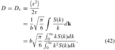
Matthaeus et al. (1995) pointed out that the integral in Equation (31) introduces a new length scale, the ultrascale  . That equation can be expressed as (Ruffolo et al. 2004)
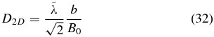
with
These concepts can be generalized to 3D turbulence. For isotropic turbulence, the diffusion coefficients in Equations (28) and (30) can be expressed as
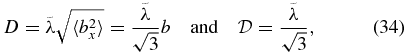
where
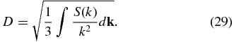
i.e.,  is the k−2 moment of the power spectrum. This form of Bohm diffusion is similar to that anticipated from our heuristic derivation (Equation (21)).
3.3. Random Ballistic Decorrelation
In the random ballistic decorrelation (RBD) version of the theory, instead of the assumption of diffusive spreading as in Equation (19), we assume that the magnetic field lines ballistically spread in random directions over the decorrelation distance. Adapted from Ghilea et al. (2011),

In the conceptual derivation, T depends on the magnitude of the local field b as

so
Since S is determined for a ballistic trajectory over a distance ℓ, we simply use
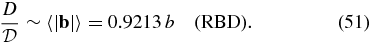
Then the ratio  for RBD is expected to be
The ratio  can help distinguish between DD and RBD, as will be discussed later in this section.
Let us turn to a full mathematical derivation of the asymptotic diffusion coefficient for RBD. With the RBD variance from Equation (36), Equation (26) becomes
Using the analogous results for the Δy and Δz integrals and  from isotropy, we obtain 〈x2〉 for large τ as
Now we can obtain the random ballistic diffusion coefficient as
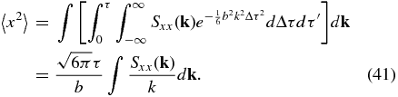
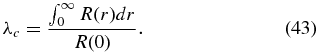
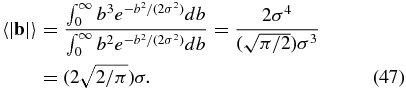
The integrals in Equation (42) are related to the total correlation length λc. To see this, first note that for an isotropic field, we can consider the total correlation function R(r) = 〈b(r0) · b(r0 + r)〉, where r0 is an arbitrary position. The correlation length is then
If we define R(r) in terms of its Fourier transform
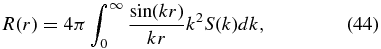
then we get R(0) = 4π∫k2S(k)dk and 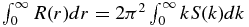 , which when combined give
A similar result for isotropic 2D turbulence was presented by Matthaeus et al. (2007). Thus we obtain
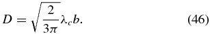
Guided by the heuristic result in Equation (37), we consider how to express Equation (46) in terms of 〈|b|〉. Assuming that the local distribution in b is Gaussian with width σ in each component, which is the case in our simulations, we have
Note that b2 = 3σ2, so  . Then
Thus we can rewrite Equation (46) in terms of 〈|b|〉 as
an expression of Bohm diffusion that is similar to the result of our heuristic derivation (Equation (37)).
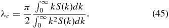
Finally, we note that DD and RBD give different predictions for  . For DD,
and for RBD,
Thus in addition to comparing D versus τ between simulations and different versions of the theory, we can compare the ratio of asymptotic values  between the simulations and DD and RBD predictions.
3.4. Evolution of the Field Line Random Walk
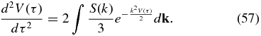
In the previous two subsections, we determined the magnetic field line diffusion coefficients in the asymptotic limit τ → ∞. Here we consider the evolution of diffusion coefficients with τ by using an ordinary differential equation (ODE). To formulate the ODE, we start by considering the running diffusion coefficient, defined by
Substituting Equation (16) into Equation (52),
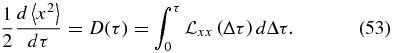
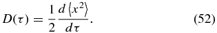
We define V(τ) = 〈x2〉, and the initial condition for Equation (53) is V(0) = 0. Then, differentiating this equation, we obtain
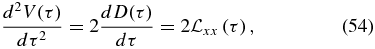
with the initial condition D(0) = 0. Assuming Corrsin's hypothesis and a Gaussian displacement distribution with variance σ2 along each coordinate, the ODE (Equation (54)) becomes
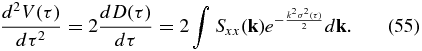
In order to determine the FLRW evolution, one can calculate the running diffusion coefficient D(τ) by integrating Equation (56) from 0 to τ. The asymptotic diffusion coefficient D is obtained by integrating to ∞. For the DD model, one can start by setting σ2(τ) = 2Dτ in Equation (56), using the asymptotic diffusion coefficient D, where τ is assumed to be positive. Then we can determine D by integrating Equation (56) over τ from 0 to ∞ and solving the resulting implicit equation for D, as in Section 3.2. After determining D, one can obtain the evolution of the DD running diffusion coefficient by integrating Equation (56) from 0 to any τ. For the RBD model, we substitute  from Equation (36) into Equation (56). Then we can determine the RBD running diffusion coefficient and RBD asymptotic diffusion coefficient by integrating Equation (56). In addition to the DD and RBD models, in Equation (56), we can identify σ2(τ) = V(τ), which provides self-closure of the ODE. We refer to this as the "ODE model," which was suggested by Saffman (1963) and Taylor & McNamara (1971), and is sometimes simply referred to in the literature as the "Corrsin approximation." We obtain a result equivalent to those obtained by Lundgren & Pointin (1976), Wang et al. (1995), Shalchi & Kourakis (2007), and Snodin et al. (2013a):
Using the definition of the diffusion coefficient in Equation (52), Equation (57) can be rewritten as a system of two first-order ODEs:
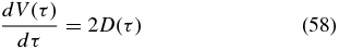
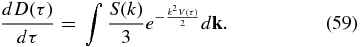
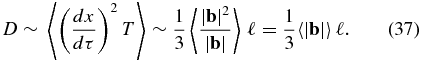
Solving Equations (58) and (59), subject to the initial conditions V(0) = 0 and D(0) = 0, the evolution of the ODE running diffusion coefficient is obtained. At low τ, we obtain V(τ)∝τ2, which is consistent with ballistic field line trajectories. One can obtain the asymptotic diffusion coefficient via a first integral, following Taylor & McNamara (1971). From Equation (57),
Multiplying by dV(τ)/dτ, we obtain
Let us consider the difference between D2(τ = ∞) and D2(τ = 0):
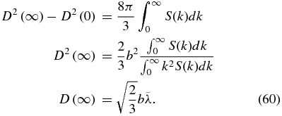
We note that this diffusion coefficient is a factor of  greater than the one obtained for DD. This factor of
  was also obtained by Snodin et al. (2013a) and Ruffolo & Matthaeus (2013) for 2D or quasi-2D axisymmetric transverse turbulence.
4. COMPUTER SIMULATIONS
4.1. Techniques and Testing
To test the validity of our analytic models of magnetic field line diffusion for isotropic turbulence with zero mean field, we performed direct computer simulations to calculate the running diffusion coefficients without using any of the assumptions of the analytic models. The isotropic 3D fluctuating magnetic field is generated on a regular Fourier grid in wave number space (k space). The solenoidal property ∇ · b = 0 in real space implies k · b(k) in wave number space. Therefore, the component b(k) at a given k is given by
where b1 and b2 are unit vectors perpendicular to each other and also to k, which ensures that the constructed field is divergence free. Here ϕ1 and ϕ2 are independent random phases at every k for these two polarization directions and S(k) is the power spectrum, given by
with a normalization constant C, used to control the magnetic field strength b, and where λ is the bendover scale. Note that for 3D isotropic fluctuations at a given magnitude k, the omnidirectional power spectrum is E(k) = 4πk2S(k), which at large k satisfies the scaling E(k)∝k−Γ. For example, when we set Γ = 5/3 we obtain the Kolmogorov scaling E(k)∝k−5/3. At low k, Equation (62) yields S(k)∝k2 as required by homogeneity (Batchelor 1970). To yield a good resolution of the discrete power spectrum, we use a zero padding technique, setting the power to zero for all k above half of the Nyquist value. Taking an inverse fast Fourier transform of b(k) yields the real space magnetic field representation. To simulate the power spectrum covering the energy containing range and the inertial range of turbulence with zero padding, we generate the 3D isotropic field for b = 1 and λ = 1 on a periodic box of size Lx = Ly = Lz = 100 with Nx × Ny × Nz = 1024 × 1024 × 1024 grid points. In this work it is interesting to note that simulation results for diffusion coefficients are essentially unchanged (at least for Γ = 5/3) if we simply use  , instead of the expression in Equation (61).
The above random prescription allows us to generate as many different realizations of a magnetic field with a given spectrum as we wish. In each realization, we trace multiple magnetic field lines, where each line is obtained by solving the system of magnetic field line equations from a random initial location, using Equations (4) up to τ = 125 and Equations (2) up to s = 125. We solve the magnetic field line equations numerically using a fifth-order Runge–Kutta method with adaptive time stepping regulated by a fourth-order error estimate step. We traced 500,000 field lines, using 12,500 lines per field representation, to help ensure sufficient sampling. Collecting displacements for all pairs of points along each field line, the running diffusion coefficients were calculated.
The theories presented earlier predict  or bλc, and
  or λc. When deriving
  and λc from the above spectrum of Equation (62), they are found to be proportional to the bendover scale λ. Therefore, one expects that the diffusion coefficients will scale proportionally with λ. As a basic test of our code, we performed simulations with various values of λ, and confirmed that D∝bλ and
  .
.
4.2. Results
We explore the effect of the power spectrum on the FLRW by considering three values of Γ corresponding to different models of magnetohydrodynamic turbulence phenomenology (for a review, see Zhou et al. 2004). These are Iroshnikov–Kraichnan scaling with Γ = 3/2 (Iroshnikov 1963; Kraichnan 1965), Kolmogorov scaling with Γ = 5/3 (Kolmogorov 1941; Batchelor 1970), and "weak turbulence" scaling with Γ = 2 (Ng & Bhattacharjee 1997; Galtier et al. 2000). The value of Γ is used to specify the power spectrum of fluctuations according to Equation (62), both in the computer simulations and for evaluation of the analytic theory.
After tracing 500,000 field lines for b = 1 and λ = 1, the running diffusion coefficients Di(τ) and  were determined, as shown in Figure 2 for the example case of Γ = 5/3. The simulations are sufficiently accurate that the estimates of diffusion coefficients in each direction are nearly coincident, according to the symmetry of the problem, indicating that a sufficient number of field lines and realizations of turbulence have been simulated. At large values of τ or s, the diffusion coefficients approach asymptotic values. For Γ = 3/2, 5/3, and 2, Table 1 shows the asymptotic diffusion coefficients D and
  , which were calculated by averaging Di(τ) and
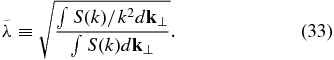
  for i = x, y, and z, weighting according to the number of available pairs of points, over the interval 60 < τ < 80 or 60 < s < 80. The error of the mean, indicated by parentheses, was determined based on the spread among the values along the three directions. Table 1 also shows the diffusion coefficients calculated for the three versions of the theory. For a more precise comparison with computer simulation results, we evaluated the integrals in Equation (33) over a finite k range, from the minimum to the maximum k values in the Fourier grid used in the simulations. Recall that all three versions of the theory predict Bohm diffusion (as generalized to the case of zero mean field in Section 2) as is usual for theories using Corrsin hypothesis at high Kubo number R. The computer simulation results confirm that for this case of R = ∞, the asymptotic diffusion coefficients are consistent with Bohm diffusion (the diffusion coefficients are finite). The simulation results are also numerically close to the results of all three versions of the Corrsin-based theory. We can see that the ratios between all asymptotic diffusion coefficients are very similar when changing the power spectral index in Equation (62) to change the omnidirectional power spectrum at high k from k−5/3 to k−3/2 or k−2, indicating that our results are not sensitive to such details of the power spectrum.
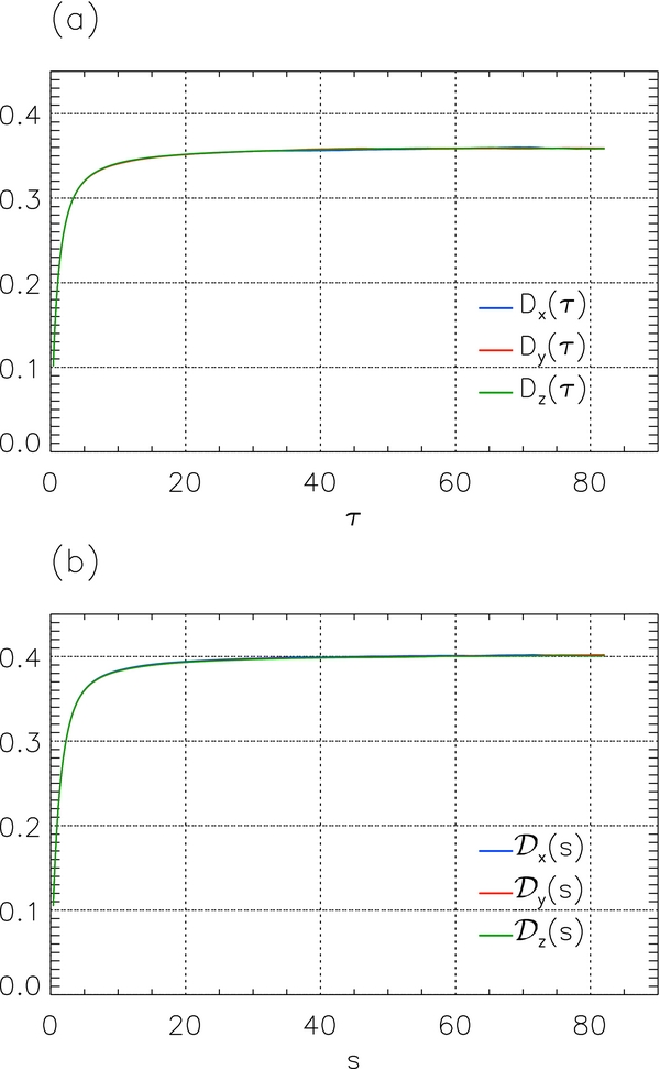
Figure 2. Magnetic field line diffusion coefficients as a function of (a) τ and (b) s from simulations of isotropic turbulence with zero mean field for the example case of Γ = 5/3 (in units of b = 1 and λ = 1). The diffusion coefficients with respect to each coordinate are in very good agreement and almost coincide.
Download figure:
Standard image High-resolution imageTable 1. Asymptotic Field Line Diffusion Coefficients and Their Ratios (b = 1, λ = 1)
| Quantity | Parameters | Evaluation | Value | ||
|---|---|---|---|---|---|
| Γ = 3/2 | Γ = 5/3 | Γ = 2 | |||
| D | τ | Theory:DD | 0.2881 | 0.3094 | 0.3522 |
| Theory:RBD | 0.2680 | 0.2916 | 0.3405 | ||
| Theory:ODE | 0.4075 | 0.4376 | 0.4981 | ||
| Simulation | 0.3357(9) | 0.3600(5) | 0.4069(7) | ||
 |
s | Simulation | 0.3759(1) | 0.3998(5) | 0.4517(9) |
D/ |
τ and s | Theory:DD | 1.0000 | 1.0000 | 1.0000 |
| Theory:RBD | 0.9213 | 0.9213 | 0.9213 | ||
| Simulation | 0.8929(24) | 0.9005(17) | 0.9008(23) | ||
Download table as: ASCIITypeset image
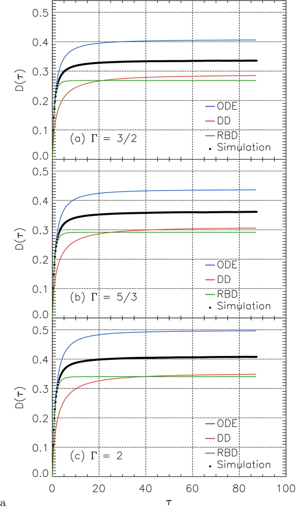
Let us now consider whether the simulation results favor a particular version of the theory. Among the DD, RBD, and ODE versions, the DD result is closest to the simulation result (DD is 14% lower). However, the evolution of running diffusion coefficients as a function of τ as shown in Figure 3 indicates that RBD is more accurate than DD in comparison with computer simulations at small τ and thus better tracks the transition from free streaming to asymptotic diffusion. Moreover, the asymptotic diffusion coefficient predicted by RBD is only slightly lower than the DD result and is 18% lower than the simulation result. In addition to comparing theory and simulation results for D(τ), we also compare the ratio of asymptotic values  between simulations and DD and RBD models. It came as a surprise that tracing the field line diffusion in τ and s at the same time can shed some light on the physical processes. After all, τ and s provide two parameterizations of the same field line trajectories. However, in the RBD calculation of diffusion coefficients, the mean free value T weights the b ensemble differently than the mean free value S, while in the DD calculation the weights are independent of the local field, so the comparison between D and
  helps indicate the dominant FLRW mechanism. The
  ratios from simulations are close to 0.90, and are much closer to the RBD prediction of 0.9213 than to the DD prediction of 1. This may indicate that the RBD version best captures the physics of the FLRW in addition to being physically simplest and easiest to implement.
Figure 3. Magnetic field line diffusion coefficient as a function of τ from simulation (using the average of the three lines shown in Figure 2(a)) and three versions of the analytic theory for b = 1, λ = 1, and different choices for the spectral index of the fluctuation power spectrum: (a) Γ = 3/2, (b) Γ = 5/3, and (c) Γ = 2.
Download figure:
Standard image High-resolution image
5. DISCUSSION AND CONCLUSIONS
In the present work, we have examined the FLRW for isotropic magnetic turbulence with a zero mean field (B0 = 0). In terms of the Kubo number R = (b/B0)(ℓ∥/ℓ⊥), this represents a limiting case of R = ∞. Most previous works considered bz = 0 or bz ≪ B0, in which case R → ∞ is a quasi-2D limit. In that quasi-2D route to R → ∞, theories based on Corrsin's hypothesis have been found to deviate from direct simulation results because of trapping effects (e.g., Vlad et al. 1998; Ghilea et al. 2011). Our work considers a different route to R = ∞ and is thus of complementary theoretical interest. Isotropic magnetic turbulence with no mean field is also of astrophysical relevance for modeling interstellar turbulence.
A key issue in studying such turbulence, where bz is not negligible compared with B0, is that the FLRW can no longer be parameterized in terms of the Cartesian coordinate z along B0. We have developed parameterizations in terms of the arclength s and in terms of τ such that dτ = ds/B, where B is the magnitude of the total magnetic field. The latter is well suited to a theoretical description. We have worked out the analogs to quasilinear, Bohm, and percolative diffusion. For B0 = 0 and parameterizing in terms of either s or τ, a quasilinear field line diffusion coefficient would diverge, a Bohm coefficient would remain finite, and a percolative coefficient would tend to zero. In other words, the FLRW would be superdiffusive, diffusive, or subdiffusive, respectively. A finite diffusion coefficient is only possible for Bohm diffusion.
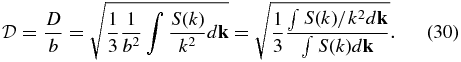
We have developed theories for the field line diffusion coefficient D(τ) based on Corrsin's hypothesis. As is usual for Corrsin-based theories at high Kubo number, they predict Bohm diffusion and hence a finite diffusion coefficient for B0 = 0. They yield an asymptotic diffusion coefficient D ∼ bℓ, where ℓ is a coherence scale of the turbulence. In particular, we obtain expressions in terms of the correlation scale λc (from the k−1 moment of the power spectrum) or the ultrascale  (from the k−2 moment).
By performing direct computer simulations, we have confirmed Bohm diffusion for isotropic magnetic turbulence with a zero mean field. Broadly speaking, all three versions of the theory give asymptotic diffusion coefficients D that are close to the simulation value (within 25%) for a fluctuation spectrum with Γ = 3/2, 5/3, or 2. The good agreement for various Γ values indicates that the theory has some power of generalization. While DD gives a D value that is slightly closer to simulations, there is little difference from the RBD prediction (see Table 1). Figure 3 compares the evolution of D(τ) for the DD, RBD, and ODE versions of theory and the simulation results, and the comparison is consistent with those of previous work on other types of turbulence (Snodin et al. 2013a, 2013b): RBD (assuming ballistic trajectories) fits better at early τ, DD (assuming diffusive trajectories) provides a better match to the later evolution, and ODE overestimates the diffusion coefficient for non-quasilinear cases such as the present work. We also compare the ratio of asymptotic diffusion coefficients for the two parameterizations,  , for simulation and theory results, which seems to favor RBD as a better description of the physical process of field line diffusion. The RBD version was also the version that performed best at high Kubo numbers for noisy RMHD turbulence (Snodin et al. 2013b).
Our overall conclusions are that Corrsin-based theories remain applicable along this route to high Kubo numbers, and limitations found in previous work with bz ≪ B0 were due to the quasi-2D limit and resulting trapping effects, not the high Kubo number per se. For astrophysical applications, the field line diffusion coefficient can be scaled from our simulation results, and for physical understanding and theoretical modeling, the RBD model based on random ballistic trajectories is simple to apply and best captures the physics.
W.S. and D.R. thank the University of Delaware for their hospitality while part of this work was carried out. This research was partially supported by a study grant from the Panyapiwat Institute of Management, the Thailand Research Fund, the US National Science Foundation under the Solar-Terrestrial research program (AGS-1063439) and the SHINE program (AGS-1156094), NASA under the Heliospheric Theory Program (NNX11AJ44G), the Solar Probe Plus/ISIS Project, a Postdoctoral Fellowship from Mahidol University, and a Sritrangthong Scholarship from the Faculty of Science, Mahidol University. We thank the anonymous reviewer for useful suggestions to improve the breadth and clarity of our work.