


ABSTRACT
We analyzed light curves of seven relatively slower novae, PW Vul, V705 Cas, GQ Mus, RR Pic, V5558 Sgr, HR Del, and V723 Cas, based on an optically thick wind theory of nova outbursts. For fast novae, free–free emission dominates the spectrum in optical bands rather than photospheric emission, and nova optical light curves follow the universal decline law. Faster novae blow stronger winds with larger mass-loss rates. Because the brightness of free–free emission depends directly on the wind mass-loss rate, faster novae show brighter optical maxima. In slower novae, however, we must take into account photospheric emission because of their lower wind mass-loss rates. We calculated three model light curves of free–free emission, photospheric emission, and their sum for various white dwarf (WD) masses with various chemical compositions of their envelopes and fitted reasonably with observational data of optical, near-IR (NIR), and UV bands. From light curve fittings of the seven novae, we estimated their absolute magnitudes, distances, and WD masses. In PW Vul and V705 Cas, free–free emission still dominates the spectrum in the optical and NIR bands. In the very slow novae, RR Pic, V5558 Sgr, HR Del, and V723 Cas, photospheric emission dominates the spectrum rather than free–free emission, which makes a deviation from the universal decline law. We have confirmed that the absolute brightnesses of our model light curves are consistent with the distance moduli of four classical novae with known distances (GK Per, V603 Aql, RR Pic, and DQ Her). We also discussed the reason why the very slow novae are about ∼1 mag brighter than the proposed maximum magnitude versus rate of decline relation.
Export citation and abstract BibTeX RIS
1. INTRODUCTION
A classical nova is a thermonuclear runaway event on a mass-accreting white dwarf (WD) in a binary. When the mass of the hydrogen-rich envelope on the WD reaches a critical value, hydrogen ignites to trigger a nova outburst. Optical light curves of novae have a wide variety of timescales and shapes (e.g., Payne-Gaposchkin 1957; Duerbeck 1981; Strope et al. 2010; Hachisu & Kato 2014). Hachisu & Kato (2006) found that in terms of free–free emission, optical and near-infrared (NIR) light curves of several novae follow a universal decline law. Their time-normalized light curves are almost independent of the WD mass, chemical composition of ejecta, and wavelength. Hachisu & Kato (2006) also found that their UV 1455 Å model light curves (Cassatella et al. 2002), interpreted as photospheric blackbody emission, are also time-normalized by the same factor as in the optical and NIR light curves. Using the fact that the time-scaling factor is closely related to the WD mass, the authors determined the WD mass and other parameters for a number of well-observed novae (e.g., Hachisu & Kato 2007, 2010, 2014; Hachisu et al. 2008; Kato et al. 2009).
On the basis of the universal decline law, Hachisu & Kato (2010) further obtained absolute magnitudes of their model light curves and derived their maximum magnitude versus rate of decline (MMRD) relation. Such MMRD relations were empirically proposed, e.g., by Schmidt (1957), della Valle & Livio (1995), and Downes & Duerbeck (2000). For individual novae, however, there is large scatter around the proposed trends (e.g., Downes & Duerbeck 2000). Hachisu & Kato's (2010) theoretical MMRD relation is governed by two parameters; one is the WD mass, and the other is the initial envelope mass at the nova outburst, i.e., the ignition mass. The ignition mass depends on the mass-accretion rate to the WD: the higher the mass-accretion rate, the smaller the ignition mass (e.g., Nomoto 1982; Prialnik & Kovetz 1995; Kato et al. 2014), i.e., the smaller the mass-accretion rate, the brighter the maximum magnitude. They therefore concluded that this second parameter (the ignition mass) explains scatter of the MMRD distribution of individual novae from the averaged trend that was determined mainly by the WD mass. Thus, the main trends of nova speed class were theoretically clarified.
In this way, the main properties of fast novae have been theoretically explained, in which free–free emission dominates the continuum spectra in optical and NIR bands. As far as free–free emission is the dominant source of nova optical light curves, there should be the universal decline law, and we expect that novae follow Hachisu & Kato's (2010) theoretical MMRD relation, with the intrinsic scatter mentioned above. For slow novae, however, the universal decline law could not be applied because photospheric emission contributes substantially to the continuum spectra rather than free–free emission (Hachisu & Kato 2014). Our aim for this paper is to analyze light curves of seven relatively slower novae, PW Vul, V705 Cas, GQ Mus, RR Pic, V5558 Sgr, HR Del, and V723 Cas, and to clarify how their light curves deviate from the universal decline law.
We organize the present paper as follows. Section 2 describes our strategy of light curve analysis. In Section 3, we start with a study of well-observed multiwavelength light curves of the slow nova PW Vul, and, through our method, we determine its relevant physical parameters, such as the WD mass. Our method for nova light curves is also applied to the moderately fast nova, V705 Cas, in Section 4; to the fast nova, GQ Mus, in Section 5; and to the very slow novae, RR Pic, V5558 Sgr, HR Del, and V723 Cas, in Section 6. Discussion and conclusions follow in Sections 7 and 8. Appendix A is devoted to a calibration of the absolute magnitude of our free–free model light curves and a theoretical MMRD relation. Appendix B presents our time-stretching method for PW Vul.
2. ANALYSIS ON VARIOUS LIGHT CURVE SHAPES OF CLASSICAL NOVAE
Figure 1 shows optical light curves of our target novae, V723 Cas, HR Del, V5558 Sgr, RR Pic, GQ Mus, PW Vul, and V705 Cas, on a linear timescale. These seven novae are plotted in the order of global decline rate. The light curves show a rich variety of shapes; one might therefore think that there are no common physical properties, such as the universal decline law. However, we can find common properties hidden in the complicated light curve shapes. For example, PW Vul shows an oscillatory behavior in the light curve, but the overall decline trend and color evolution are very similar to other smoothly declining classical novae, as shown in Figure 2 (see Section 3 for details). Figure 2 depicts the time-normalized light curves of PW Vul and well-observed fast novae. Figures 3 and 4 also show the light curves and colors of V723 Cas, HR Del, V5558 Sgr, and RR Pic. Looking closely at the light curves in Figures 2–4, we can see common properties as follows.
- 1.
- 2.
- 3.
- 4.The UV 1455 Å narrow-band flux basically follows a time-normalized universal shape unless the flux is absorbed by dust. The theoretical flux (solid red line) represents a blackbody flux of the pseudophotosphere (Kato & Hachisu 1994).

Figure 1. Visual and V light curves for seven novae, from top to bottom, V723 Cas, HR Del, V5558 Sgr, RR Pic, GQ Mus, PW Vul, and V705 Cas, in the order of global decline rates. Red or blue open circles denote V magnitudes for each nova. Green filled triangles are J, blue open squares are H, and magenta open triangles are K magnitudes of PW Vul. Their reference sources are found in the section of each object. Red or blue small dots represent visual magnitudes, all taken from the American Association of Variable Star Observers (AAVSO) archive except for GQ Mus. Small blue dots for GQ Mus are visual magnitude data collected by the Royal Astronomical Society of New Zealand. A solid blue line is our theoretical free–free emission light curve for a 0.83 M☉ WD (see Section 3), which nicely fits with the near-infrared (NIR) light curves of PW Vul but not with the optical data that is contaminated by strong emission lines in the nebular phase.
Download figure:
Standard image High-resolution image
Figure 2. (a) V-band and UV 1455 Å narrow-band light curves, (b) (B − V)0, and (c) (U − B)0 color curves, for PW Vul (magenta open circles with plus sign inside), V1500 Cyg (red open diamonds), V1668 Cyg (black filled squares), and V1974 Cyg (green open and filled triangles). The reference sources are the same as those in Hachisu & Kato (2006, 2010, 2014). Here, (B − V)0 and (U − B)0 denote dereddened colors. Each color is dereddened with (B − V)0 = B − V − E(B − V) and (U − B)0 = U − B − 0.64E(B − V) (Rieke & Lebofsky 1985). Those of V533 Her are also added: blue filled circles are taken from van Genderen (1963), blue open circles are from Chincarini (1964), and blue star symbols are from Shen et al. (1964). To make them overlap in the early decline phase, we horizontally shift their logarithmic times of PW Vul, V1668 Cyg, V1974 Cyg, and V533 Her by −0.74 = log 0.182, −0.36 = log 0.44, −0.38 = log 0.42, and −0.28 = log 0.54, and vertically shift their magnitudes by −2.6, −2.9, −0.8, and +0.8 mag, respectively, as indicated in the figure. The UV 1455 Å fluxes of each nova are also rescaled against that of V1668 Cyg, as indicated in the figure. Here, we assume the start of the day (t = 0) as JD 2445910.0 for PW Vul and JD 2438052.0 for V533 Her to correctly overlap them with other light curves. Solid red lines are our theoretical free–free emission and UV 1455 Å light curves for a 0.83 M☉ WD (see Section 3). We also draw two red horizontal lines of (b) B − V = −0.03 and (c) U − B = −0.97, both of which are the colors of optically thick free–free emission (see, e.g., Hachisu & Kato 2014).
Download figure:
Standard image High-resolution image
Figure 3. (a) Visual, V-band, and UV 1455 Å narrow-band light curves and (b) (B − V)0 and (c) (U − B)0 color curves for RR Pic (magenta open circles with plus sign inside, magenta dots), V723 Cas (red open and filled triangles, red dots), HR Del (blue open stars, open circles, filled circles, blue dots), and V5558 Sgr (green open and filled squares, green dots). Here, (B − V)0 and (U − B)0 denote dereddened colors. To make them overlap in the early decline phase, we horizontally shift their times and vertically shift their magnitudes by +5.3, 0.0, +3.6, and +0.1 mag, respectively, as indicated in the figure. UV 1455 Å fluxes of V723 Cas are plotted by large open circles. Solid black/red lines are our theoretical V/UV 1455 Å light curves for a 0.51 M☉ WD (see Section 6.4). We add two red horizontal lines of (b) B − V = +0.13 and (c) U − B = −0.82, both of which are the colors of optically thin free–free emission (see, e.g., Hachisu & Kato 2014).
Download figure:
Standard image High-resolution image
Figure 4. Same as Figure 3, but on a logarithmic timescale.
Download figure:
Standard image High-resolution imageNovae blow optically thick winds, which are the origin of free–free emission. As far as the free–free emission dominates the continuum spectra, we can expect that novae follow the universal decline law. Even if there are wavy structured or dust blackout shapes, the overall light curves follow the universal decline law (e.g., Hachisu & Kato 2006, 2007, 2010, 2014; Hachisu et al. 2008; Kato et al. 2009). On the other hand, if photospheric emission dominates the nova continuum spectra, light curves do not follow the universal decline law.
Figure 5 shows a schematic illustration of nova continuum spectrum superposed on the various wavelength bands. Free–free spectra are plotted for a high wind mass-loss rate (solid red line) and a low wind mass-loss rate (solid blue line). In general, slower novae are related to less massive WDs, which blow optically thick winds with relatively smaller wind mass-loss rates (Kato & Hachisu 1994). Thus, in such cases, we apply the universal decline law only to light curves in the NIR region but not to light curves in the optical regions.

Figure 5. Illustrative example of spectral energy distribution of a classical nova with a photospheric temperature of Tph = 50, 000 K, as well as passbands of the photometric filters used in this work. The UV 1455 Å (1445–1465 Å) and supersoft X-ray (0.1–2.4 keV) fluxes are calculated from blackbody spectrum while the U, V, J, and K magnitudes are calculated from the free–free emission spectrum. Note that the flux of free–free emission depends on the wind mass-loss rate,  . If the mass-loss rate is large, the flux of free–free emission dominates the spectrum in the optical and IR regions, as indicated by a solid red line. If it is small, the flux of free–free emission may dominate only in the IR region, as indicated by a blue line. The supersoft X-ray flux is negligibly small for the adopted photospheric temperature.
Download figure:
Standard image High-resolution imageIn this paper, we analyze the light curves of relatively slower novae in the following way.
- 1.First, we determine the WD mass by applying properties (1)–(4) above.
- 2.For this specified WD mass, we calculate the composite light curve of free–free plus photospheric emissions. From the fitting with the V data, we determine the V-band distance modulus of (m − M)V. We further estimate the distance to the nova if the color excess E(B − V) is known.
- 3.We compare our results with various properties in literature.
We first analyze PW Vul, V705 Cas, and GQ Mus based on the method mentioned above. These are the three novae in the lower part of Figure 1. We then look at the other four novae, RR Pic, V5558 Sgr, HR Del, and V723 Cas. These four novae show more or less similar light curves in their optical maximum and decline phases, as shown in Figures 1, 3, and 4.
3. PW Vul 1984#1
PW Vul (Nova Vulpeculae 1984#1) was discovered by Wakuda on UT 1984 July 27.7 (Kosai et al. 1984) about a week before its optical maximum of mV, max = 6.3 on UT 1984 August 4.1. The light curve is plotted in Figure 1 on a linear timescale and in Figure 2 on a logarithmic timescale. The X-ray flux increased during the first year (Öegelman et al. 1987) and faded before the ROSAT observation (1990–1999). No X-ray data are available in the supersoft X-ray phase.
3.1. Reddening and Distance
Andreae et al. (1991) obtained E(B − V) = 0.58 ± 0.06 from the He ii λ1640/λ4686 ratio and E(B − V) = 0.55 ± 0.1 from the interstellar absorption feature at 2200 Å for the reddening toward PW Vul. Saizar et al. (1991) reported E(B − V) = 0.60 ± 0.06 from the He ii λ1640/λ4686 ratio. Duerbeck et al. (1984) estimated the extinction to be E(B − V) = 0.45 ± 0.1 from galactic extinction in the direction toward the nova, whose galactic coordinates are (l, b) = (61 0983, +51967). For the galactic extinction, we examined the galactic dust absorption map in the NASA/IPAC Infrared Science Archive,3 which is calculated on the basis of recent data from Schlafly & Finkbeiner (2011). It gives E(B − V) = 0.43 ± 0.02 in the direction of PW Vul. The arithmetic mean of these four values is E(B − V) = 0.55 ± 0.05.
Recently, Hachisu & Kato (2014) proposed a new method for determining reddening of classical novae. They identified a general course of UBV color–color evolution and determined reddenings of novae by matching the track of a target nova with their general course. They obtained E(B − V) = 0.55 ± 0.05 for PW Vul, which agrees well with the above mean value.
As for the distance to PW Vul, a reliable estimate, d = 1.8 ± 0.05 kpc, was obtained by Downes & Duerbeck (2000) through the nebular expansion parallax method. Adopting this value, together with E(B − V) = 0.55 ± 0.05, the distance modulus of PW Vul is

We also obtained (m − M)V, PWVul = 13.0 ± 0.1 (see Appendix B) from "the time-stretching method" (Hachisu & Kato 2010) of nova light curves. This value is consistent with Equation (1).
Figure 6 shows various distance-reddening relations for comparison. A horizontal magenta thick solid line with flanking thin lines represents the distance estimate of d = 1.8 ± 0.05 kpc (Downes & Duerbeck 2000) mentioned above. A vertical solid black line with flanking thin lines represents the color excess of E(B − V) = 0.55 ± 0.05. The distance-reddening relation of Equation (1) is plotted by a thick solid blue line with flanking thin solid lines.

Figure 6. Distance-reddening relation toward PW Vul. Thick solid blue line with flanking thin solid lines denotes the distance-reddening relation calculated from the distance modulus of Equation (1), i.e., (m − M)V = 5log (d/10 pc) + 3.1E(B − V) = 13.0 ± 0.2. Vertical thick solid black line with flanking thin lines represents the color excess of E(B − V) = 0.55 ± 0.05. Horizontal thick solid magenta line with flanking thin lines represents the distance estimate of d = 1.8 ± 0.05 kpc from an expansion parallax method (Downes & Duerbeck 2000). Distance-reddening relations in four directions close to PW Vul are shown by four different sets of data with error bars, taken from Marshall et al. (2006), i.e., (l, b) = (6100, 500) (red open squares), (6125, 500) (green filled squares), (6100, 525) (blue asterisks), and (6125, 525) (magenta open circles). Typical error bars are shown by only two points for each set to avoid complexity of lines.
Download figure:
Standard image High-resolution imageMarshall et al. (2006) published a three-dimensional dust extinction map of our galaxy in the direction of −1000 ⩽ l ⩽ 1000 and −100 ⩽ b ⩽ +100, with grids of Δl = 025 and Δb = 025, where (l, b) are the galactic coordinates. Four sets of data with error bars in Figure 6 show distance-reddening relations in four directions close to PW Vul: (l, b) = (6100, 500) (red open squares), (6125, 500) (green filled squares), (6100, 525) (blue asterisks), and (6125, 525) (magenta open circles). The closest one is the blue asterisk relation, which gives E(B − V) = 0.42 ± 0.08 at d ≈ 1.8 ± 0.05 kpc. This value is consistent with E(B − V) = 0.43 ± 0.02 calculated from the NASA/IPAC dust map in the direction of PW Vul. Our value of E(B − V) = 0.55 obtained above is larger than these values. However, the reddening trend of blue asterisks suggests a large deviation from the other three trends by ΔE(B − V) ≈ 0.1, i.e., reddening has patchy structure in this direction, and further variation of ΔE(B − V) ∼ 0.1 is possible. Thus, we adopt E(B − V) = 0.55 and d ≈ 1.8 kpc in this paper.
3.2. Chemical Composition of Ejecta
One of the most intriguing properties of classical novae is the metal enrichment of ejecta (e.g., Gehrz et al. 1998), which is ascribed to mixing with WD core material during outburst (e.g., Prialnik & Kovetz 1995). PW Vul is not an exception to this general trend, as summarized in Table 1. There is a noticeable scatter in the abundance estimates, from X = 0.47 to X = 0.69. The arithmetic mean is X = 0.57, Y = 0.22, and XCNO = 0.19 for Z = 0.02. Here, X, Y, Z, and XCNO are hydrogen, helium, heavy elements with solar abundance, and carbon–nitrogen–oxygen fractions in weight, respectively.
Table 1. Chemical Composition of Selected Novae
| Object | H | CNO | Ne | Na–Fe | Reference |
|---|---|---|---|---|---|
| HR Del 1967 | 0.45 | 0.074 | 0.0030 | ⋅⋅⋅ | Tylenda (1978) |
| DQ Her 1934 | 0.27 | 0.57 | ⋅⋅⋅ | ⋅⋅⋅ | Petitjean et al. (1990) |
| DQ Her 1934 | 0.34 | 0.56 | ⋅⋅⋅ | ⋅⋅⋅ | Williams et al. (1978) |
| V705 Cas 1993 #2 | 0.57 | 0.25 | ⋅⋅⋅ | 0.0009 | Arkhipova et al. (2000) |
| V723 Cas 1995 | 0.52 | 0.064 | 0.052 | 0.042 | Iijima (2006) |
| GQ Mus 1983 | 0.37 | 0.24 | 0.0023 | 0.0039 | Morisset & Péquignot (1996) |
| GQ Mus 1983 | 0.27 | 0.40 | 0.0034 | 0.023 | Hassall et al. (1990) |
| GQ Mus 1983 | 0.43 | 0.19 | ⋅⋅⋅ | ⋅⋅⋅ | Andreae & Drechsel (1990) |
| RR Pic 1925 | 0.53 | 0.032 | 0.011 | ⋅⋅⋅ | Williams & Gallagher (1979) |
| PW Vul 1984 #1 | 0.69 | 0.066 | 0.00066 | ⋅⋅⋅ | Saizar et al. (1991) |
| PW Vul 1984 #1 | 0.47 | 0.30 | 0.0040 | 0.0048 | Andreä et al. (1994) |
| PW Vul 1984 #1 | 0.62 | 0.13 | 0.001 | 0.0027 | Schwarz et al. (1997) |
| PW Vul 1984 #1 | 0.49 | 0.28 | 0.0019 | ⋅⋅⋅ | Andreae & Drechsel (1990) |
Download table as: ASCIITypeset image
We took a simple parameterization for the degree of mixing between core material and accreted matter as ηmix = (0.7/X) − 1. Here we assume the solar composition for the accreted matter. Table 2 shows seven representative cases of degree of mixing, i.e., 100% (denoted by "CO nova 1," "CO nova 2," and "Ne nova 1"), 55% ("CO nova 3"), 25% ("CO nova 4" and "Ne nova 2"), and 8% ("Ne nova 3"). We first adopt "CO nova 4" because it is closest to the above averaged values of PW Vul. Then, we discuss the dependence of light curves on the chemical composition.
Table 2. Chemical Composition of the Present Models
| Novae Case | X | Y | XCNO | XNe | Za | Mixingb | Comments |
|---|---|---|---|---|---|---|---|
| CO nova 1 | 0.35 | 0.13 | 0.50 | 0.0 | 0.02 | 100% | DQ Her |
| CO nova 2c | 0.35 | 0.33 | 0.30 | 0.0 | 0.02 | 100% | GQ Mus |
| CO nova 3 | 0.45 | 0.18 | 0.35 | 0.0 | 0.02 | 55% | V1668 Cyg |
| CO nova 4 | 0.55 | 0.23 | 0.20 | 0.0 | 0.02 | 25% | PW Vul |
| Ne nova 1 | 0.35 | 0.33 | 0.20 | 0.10 | 0.02 | 100% | V351 Pup |
| Ne nova 2d | 0.55 | 0.30 | 0.10 | 0.03 | 0.02 | 25% | V1500 Cyg |
| Ne nova 3 | 0.65 | 0.27 | 0.03 | 0.03 | 0.02 | 8% | QU Vul |
| Solar | 0.70 | 0.28 | 0.0 | 0.0 | 0.02 | 0% |
Notes. aCarbon, nitrogen, oxygen, and neon are also included in Z = 0.02 with the same ratio as the solar composition (Grevesse & Anders 1989). bMixing between the helium layer + core material and the accreted matter with solar composition, which is calculated from ηmix = (0.7/X) − 1. cFree–free light curves for this chemical composition are tabulated in Table 2 of Hachisu & Kato (2010). dFree–free light curves for this chemical composition are tabulated in Table 3 of Hachisu & Kato (2010).
Download table as: ASCIITypeset image
3.3. Contribution from Photospheric Emission
We now analyze the spectra of PW Vul, assuming that the continuum flux Fν is simply the sum of a blackbody spectrum of the temperature Tph and an optically thick free–free emission with the electron temperature of Te, i.e.,

where ν is the frequency, Bν(Tph) is the Planckian of the photospheric temperature Tph = TBB, and Sν(Te) is the free–free spectrum of the electron temperature Te; f1 and f2 are numeric constants (e.g., Nishimaki et al. 2008). Following Wright & Barlow (1975), the free–free spectrum can be expressed as

where the linear free–free absorption coefficient Kν(Te) is given by

in cgs units; gν(Te) is the Gaunt factor. In general, the Gaunt factor depends weakly on the frequency and temperature, but we assume it to be unity, following Hachisu & Kato (2014). Therefore, there are four fitting parameters, i.e., f1, f2, Tph = TBB, and Te. When hν ≪ kTe, Equation (3) can be expressed as (Wright & Barlow 1975)

where 1 Jy =10−26 W m−2 Hz−1; the ion number density is assumed equal to the total gas number density, n, and the electron number density is equal to γ times the ion number density;  is the wind mass-loss rate in units of M☉ yr−1; D is the distance in units of kiloparsecs; v∞ is the terminal wind velocity in units of km s−1; μ is the mean molecular weight; Z is the charged degree of ion (only in this formula); ν is the frequency in units of Hz; and g is the Gaunt factor. Equation (5) can be further simplified as

where λ is the wavelength.
Figure 5 schematically shows the contributions of Bλ and Sλ. When the wind mass-loss rate is small, contribution of free–free emission is relatively small in Equation (2). Hachisu & Kato (2014) decomposited the spectrum of PW Vul about 64 days after the outburst using Equation (2) and concluded that the free–free flux is comparable to the pseudophotospheric flux in the V band. Here, we reanalyzed the same data and showed them in Figure 7, assuming four different extinctions, i.e., (1) E(B − V) = 0.45, (2) E(B − V) = 0.50, (3) E(B − V) = 0.55, and (4) E(B − V) = 0.60. In our decomposition process, we simply assume that TBB = Te and change the temperature in steps of 1000 K. We see that the blackbody emission gives a good approximation to the UV region, and the free–free emission is a good fit to the IR region. In the region between them, we have a comparable contribution from the blackbody and free–free components.

Figure 7. Dereddened spectrum of PW Vul, 64 days after the outburst (UT 1984 Septemebr 30 = JD 2 445 973.5) for different extinctions: (a) E(B − V) = 0.45, (b) E(B − V) = 0.50, (c) E(B − V) = 0.55, and (d) E(B − V) = 0.60. Solid red line: IUE spectra, SWP24088 and LWP04458, are taken from the INES data archive server. Open red circles: UBVRI data from Robb & Scarfe (1995) and JHKLM data from Gehrz et al. (1988). Global features of the spectrum can be fitted with a combination (thick solid black line) of the blackbody with a temperature of (a) TBB = 22, 000 K, (b) TBB = 25, 000 K, (c) TBB = 27, 000 K, and (d) TBB = 29, 000 K (thick magenta line) and the optically thick, free–free emission with the same electron temperature of Te (thick blue line). We also add a straight thin solid red line of Fλ∝λ−2.67, which corresponds to Equations (5) and (6), as the limiting case of Te = ∞ for optically thick free–free emission.
Download figure:
Standard image High-resolution imageThese four decompositions of different sets of Te = TBB and E(B − V) more or less show similarly good agreement. Among these four cases, TBB = 27, 000 K in Figure 7(c) is in best agreement with the temperature deduced from the light curve analysis in Section 3.4. It should be noted that the dereddened spectrum with E(B − V) = 0.55 is closest to the straight line (thin solid red line) of Fλ∝λ−2.67 of Equation (6). Hauschildt et al. (1997) calculated synthetic NLTE nova spectra (see their Figure 10), in which the continuum flux has a slope of Fλ∝λ−2.7 in the range of λ = 0.2–2 μm for Teff = 25, 000 K and Teff = 30, 000 K. If we apply this slope directly to PW Vul, the spectrum is in best agreement with the reddening of E(B − V) = 0.55 in Figure 7(c).
The decomposition in Figure 7(c) indicates that the photospheric emission may substantially contribute in the optical light curve. In the next subsection, we calculate theoretical light curves from the sum of free–free plus photospheric emission for the optical bands and from photospheric emission alone for the UV 1455 Å band.
3.4. Model Light Curves of "CO Nova 4"
We now make light curve models for PW Vul, assuming the chemical composition of "CO Nova 4." We calculated nova light curves for various WD masses and fitted them to the observational data. The flux in the UV 1455 Å band (a narrow band of 1445–1465 Å, see Cassatella et al. 2002) was calculated as blackbody emission from the nova pseudophotosphere (Rph and Tph), using the optically thick wind solutions in Kato & Hachisu (1994). In our fitting process, we changed the WD mass from 0.80 M☉ to 0.90 M☉ in steps of 0.01 M☉. In Figure 8, the 0.83 M☉ WD model (thin solid black lines) shows reasonable agreement with the optical, NIR, and UV observations, in particular with the UV 1455 Å observations. An arrow labeled "spectral energy distribution (SED)" indicates the date (Day 64) at which the spectrum in Figure 7 was secured. Our 0.83 M☉ WD model has Tph = 28, 000 K on this day, which is consistent with the blackbody temperature of TBB = 27, 000 K determined in Section 3.3.

Figure 8. Optical, NIR, and UV 1455 Å light curves of PW Vul. Here, we assume the start of the day (t = 0) as JD 2445897.0. Red asterisks represent V magnitudes, which were taken from IAU Circular Nos. 3971 and 4091 as well as from Robb & Scarfe (1995) and the AAVSO archive. Orange open circles with plus sign inside denote R magnitudes shifted down by 0.8 mag, taken from Robb & Scarfe (1995). Magenta open diamonds are I magnitudes shifted down by 0.7 mag, taken from Evans et al. (1990), Gehrz et al. (1988), Robb & Scarfe (1995), and Williams et al. (1991). Green filled triangles are J magnitudes shifted down by 1.6 mag, taken from Evans et al. (1990), Gehrz et al. (1988), and Williams et al. (1996). Blue open squares are H magnitudes shifted down by 1.8 mag, taken from Evans et al. (1990), Gehrz et al. (1988), Robb & Scarfe (1995), and Williams et al. (1996). Magenta open circles are K magnitudes shifted down by 2.2 mag, taken from Evans et al. (1990), Gehrz et al. (1988), and Williams et al. (1996). Large black open circles are the UV 1455 Å fluxes observed with IUE, taken from Cassatella et al. (2002). We plot three different WD mass models, 0.80 M☉ (solid blue/magenta lines), 0.85 M☉ (thick solid blue/magenta lines), and 0.90 M☉ (blue/magenta dash-dotted lines), for the envelope chemical composition of "CO nova 4." We also added a fine-mass model of 0.83 M☉ (thin solid black lines). Optically thick winds stopped about 620 days after the outburst for the case of 0.83 M☉ WD. The spectrum in Figure 7 was secured at the day denoted by an arrow labeled "SED."
Download figure:
Standard image High-resolution imageFrom the UV 1455 Å light curve fitting of the 0.83 M☉ WD in Figure 8, we obtained the following distance-reddening relation, i.e.,

where  erg cm−2 s−1 Å−1 is the calculated UV 1455 Å band flux at maximum of the 0.83 M☉ WD model for an assumed distance of 10 kpc, and
  erg cm−2 s−1 Å−1 is the maximum observed flux (Cassatella et al. 2002). Here we assume an absorption of Aλ = 8.3 × E(B − V) at λ = 1455 Å (Seaton 1979). The distance-reddening relation of Equation (7) is plotted by solid magenta lines in Figure 9 (labeled "UV 1455 Å"). Two relations of Equations (1) and (7) cross each other at the point of (E(B − V), d) = (0.57 ± 0.05 mag, 1.75 ± 0.3 kpc), consistent with the observations summarized in Section 3.1. Therefore, we safely conclude that the WD mass of PW Vul is as massive as ∼0.83 M☉ if the chemical composition is close to X = 0.55, Y = 0.23, Z = 0.02, and XCNO = 0.20.

Figure 9. Same as Figure 6, but for the 0.83 M☉ WD model with the chemical abundance of "CO nova 4." Solid blue line with flanking thin solid lines: distance-reddening relation calculated from Equation (1), labeled "(m − M)V = 13.0 ± 0.2." Solid magenta line with flanking thin solid lines: distance-reddening relation calculated from Equation (7), i.e., the UV 1455 Å flux fitting (labeled "UV 1455 Å ") of the 0.83 M☉ WD model.
Download figure:
Standard image High-resolution imageContrary to the UV 1455 Å blackbody flux, our free–free model light curves are not yet calibrated. Optical light curves in Figure 8 are freely shifted in the vertical direction to fit the observation because the proportionality constant in Equation (9) of Hachisu & Kato (2006) is unknown for "CO nova 4." To fix the absolute magnitude of each light curve, we use the absolute magnitude of PW Vul as follows.
First, we calculate the light curve model of the 0.83 M☉ WD and obtain the blackbody light curve in the V band (solid green line labeled "BB"), as shown in Figure 10. Here, we adopt the distance modulus of (m − M)V = 13.0. Assuming a trial value for the proportionality constant C in Equation (A1) of Appendix A.1, which is the same as Equation (9) of Hachisu & Kato (2006), we obtain the absolute magnitude of the free–free model light curve (solid black line labeled "FF"). The total flux (solid red line labeled "TOTAL") is the sum of these two fluxes. However, in general, this total V-magnitude light curve does not fit well with the observed data. Then, we change the proportionality constant until the total V flux fits well with the observed V light curve. Figure 10 shows our final best-fit model. We directly read mw = 16.0 from Figure 10, where mw is the apparent magnitude at the end of the wind phase (open circle at the end of solid black line labeled "FF"). Then, we obtain Mw = mw − (m − M)V = 16.0–13.0 = 3.0, where Mw is the absolute magnitude of the free–free model light curve at the end of the wind phase. Thus, the proportionality constant can be specified by Mw = 3.0 of the 0.83 M☉ WD for PW Vul.

Figure 10. Same as Figure 8, but we added blackbody V magnitude (solid green line labeled "BB") and total V magnitude (solid red line labeled "TOTAL") for the distance modulus of (m − M)V = 13.0 in the V band. We determined the absolute magnitude of the free–free emission light curve (solid black line labeled "FF") by Mw = 3.0, i.e., mw = 3.0 + 13.0 = 16.0 at the end of wind phase (denoted by a black open circle) by fitting of our model light curve of total V (solid red line) with the V observation (red asterisks). We also added visual magnitudes (blue dots), which are taken from the AAVSO archive. Our model light curve fits reasonably with the early V light curve but deviates from the visual observation in the later phase, i.e., in the nebular phase. This deviation is due to strong emission lines such as [O iii], which are not included in our model light curves. The spectrum in Figure 7 was secured at the day denoted by an arrow labeled "SED." Our 0.83 M☉ WD model shows the photospheric temperature of about Tph = 28, 000 K on this day, consistent with the fitting temperature of TBB = 27, 000 K in Figure 7. See text for more details.
Download figure:
Standard image High-resolution imageBased on the result of the 0.83 M☉ WD and applying the time-scaling law of free–free light curves to other WD mass models, we obtain the absolute magnitudes of free–free light curves for other WD masses with the chemical composition of "CO nova 4" (see Appendix A). The absolute magnitudes are specified by the value of Mw and listed in Table 4 for 0.55–1.2 M☉ WDs in steps of 0.05 M☉.
It should be noted that our model light curve fits reasonably with the early V light curve but deviates from the visual observation (small blue dots in Figure 10) in the nebular phase. On the other hand, our free–free model light curve almost perfectly fits with the NIR light curves, even in the later phase. This deviation in visual magnitudes is owing to strong emission lines, such as [O iii], which are not included in our model (see Hachisu & Kato 2006, for details). In the NIR region, free–free emission dominates the spectrum, and our free–free light curve works well.
Thus, we may conclude that the effect of photospheric emission in the V band can be neglected in novae much faster than PW Vul because the mass-loss rate is large enough for free–free emission to dominate the spectrum in the optical and NIR regions. We will discuss such examples of fast novae in Sections 7.1.1 and 7.1.2. However, in less massive WDs or in novae much slower than PW Vul, we must take into account the contribution of photospheric emission. In this sense, PW Vul lies on a border of speed class between them.
3.5. Effect of Chemical Composition
The chemical composition of ejecta is usually not so accurately constrained as described in Section 3.2 and as tabulated in Table 1. If we adopt a chemical composition different from the true one, we could miss the WD mass and distance modulus of a nova. Therefore, we examine the dependence of our model light curve on the chemical composition, i.e., the degree of mixing. We adopted two other chemical compositions of "CO nova 2," a high degree of mixing, ηmix = 1.0 (100%), and "Ne nova 2," a low degree of mixing, ηmix = 0.25 (25%), mainly because their absolute magnitudes of free–free emission model light curves were already calibrated by Hachisu & Kato (2010) independently of the light curve of PW Vul.
In a similar way to that given in Section 3.4, we have obtained best-fit models for the two chemical compositions mentioned above. Figure 11 shows our model light curves for (1) "CO Nova 2" and (2) "Ne Nova 2." In our fitting process, we changed the WD mass from 0.70 M☉ to 0.90 M☉ in steps of 0.01 M☉. In Figure 11(a), the 0.78 M☉ WD model shows reasonable agreement with the V and UV observations. Additionally, a good agreement is found for the 0.85 M☉ WD in Figure 11(b). It should be noted again that our model light curve fits well with the early V light curve but deviates from the visual observation in the later phase, i.e., in the nebular phase. This deviation is due to strong emission lines such as [O iii], which are not included in our model light curves.

Figure 11. Same as Figure 10, but for (a) the 0.78 M☉ WD model with the "CO nova 2" chemical composition and (b) the 0.85 M☉ WD model with the "Ne nova 2" chemical composition. Optically thick winds stopped (a) about 560 days and (b) about 690 days after the outburst. We obtained (a) (m − M)V = 12.8 and (b) (m − M)V = 13.2 from the total V flux fitting with the V observation.
Download figure:
Standard image High-resolution imageThe flux in the UV 1455 Å band was calculated as blackbody emission from the nova pseudophotosphere, using the optically thick wind solutions in Kato & Hachisu (1994) and Hachisu & Kato (2006, 2010). From the UV 1455 Å flux fitting, we obtained the distance-reddening relation, which is plotted by solid magenta lines (labeled "UV 1455 Å") in Figure 12. Both the distance-reddening relations of UV 1455 Å in Figure 12 are similar to that for "CO nova 4" in Figure 9.

Figure 12. Distance-reddening relation toward PW Vul for the model of (a) 0.78 M☉ WD with the chemical composition of "CO nova 2" and (b) 0.85 M☉ WD with the chemical composition of "Ne nova 2." Solid blue line with flanking thin solid lines: distance-reddening relation calculated from the fitting of total (free–free emission plus photospheric emission) V model light curve (labeled "TOTAL fit") obtained from Figure 11. Solid magenta line with flanking thin solid lines: distance-reddening relation calculated from the UV 1455 Å flux fitting (labeled "UV 1455 Å ") obtained from Figure 11. Two other constraints are also plotted; one is the distance of d = 1.8 ± 0.05 kpc determined by Downes & Duerbeck (2000) with nebular expansion parallaxes, and the other is the reddening of E(B − V) = 0.55 ± 0.05 determined from various constrains described in Section 3.1.
Download figure:
Standard image High-resolution imageThe total V fluxes are calculated from the sum of the free–free and blackbody fluxes. From the fitting, we also obtained the distance-reddening relation of (1) (m − M)V = 12.8 for the 0.78 M☉ WD and (2) (m − M)V = 13.2 for the 0.85 M☉ WD. Both are barely consistent with our adopted value of (m − M)V = 13.0 ± 0.2 for PW Vul. The two distance-reddening relations of total V-magnitude fitting are plotted by solid blue lines (labeled "TOTAL") in Figure 12. It is remarkable that our fitting misses the distance modulus only by 0.2 mag, even if we assume a different chemical composition of ΔX = 0.55–0.35 = 0.2.
For a lower value of the hydrogen content X, the evolution timescale becomes shorter, even if the WD mass is the same (see Kato & Hachisu 1994; Hachisu & Kato 2001). Therefore, a less massive WD of 0.78 M☉ is fitted with the observation for a lower value of X = 0.35, as shown in Figure 11(a). The wind mass-loss rate is smaller for a less massive WD of 0.78 M☉. The lower wind mass-loss rate leads to fainter free–free emission and, as a result, a fainter total V light curve. This is the reason for (m − M)V = 12.8, which is a bit smaller than the original value of (m − M)V = 13.0.
For the chemical composition of "Ne nova 2," however, the hydrogen content of X is the same as that of "CO nova 4." The difference is between XCNO = 0.20 and XCNO = 0.10. The CNO abundance is relevant to the nuclear burning rate, and a lower value of XCNO = 0.10 makes the evolution timescale longer. This requires a more massive WD of 0.85 M☉ than the 0.83 M☉ WD of XCNO = 0.20, as shown in Figure 11(b). The more massive WD blows stronger winds. This results in a brighter light curve of free–free emission and, as a result, a brighter total V light curve. This is the reason for (m − M)V = 13.2, which is a bit larger than the original value of (m − M)V = 13.0.
In Figure 12(a), the two distance-reddening relations, i.e., "UV 1455 Å" and "TOTAL fit," cross each other at the point of (E(B − V), d) = (0.63 mag, 1.5 kpc), not consistent with E(B − V) = 0.55 ± 0.05 and d = 1.8 ± 0.05 kpc. The degree of mixing may not be as high as 100% (X ≈ 0.35) in PW Vul.
Figure 12(b) shows that the two relations cross at the point of (E(B − V), d) = (0.54 mag, 2.0 kpc). This value is consistent with the reddening estimate of E(B − V) = 0.55 ± 0.05, although the distance estimate is a bit larger than the distance estimate of d = 1.8 ± 0.05 kpc. We may conclude that the lower degree of mixing (25% mixing) is more reasonable in PW Vul.
To summarize, we reached a reasonable distance-reddening result for a 25% mixing of "Ne Nova 2" but not for a 100% mixing of "CO Nova 2." Note that enrichment of neon with the hydrogen mass fraction being unchanged hardly influences the nova light curves because neon is not relevant to either nuclear burning (CNO cycle) or opacity (e.g., Kato & Hachisu 1994; Hachisu & Kato 2006, 2010). Therefore, the agreement in the lower 25% mixing model suggests that a lower degree of mixing (∼25%) is reasonable, rather than a higher degree of mixing (∼100%). Unfortunately, there is significant scatter in the abundance determinations (see Table 1), but their averaged values of chemical composition, which show a 23% mixing, are close enough to those of "CO nova 4." Therefore, we may conclude that through our method of model light curve fitting, one might discriminate between different degrees of mixing, at least in terms of the hydrogen mass fraction X. We summarize our fitting result for PW Pul in Table 3.
Table 3. Physical Parameters of the Present Models
| Object | WD Mass | E(B − V) | (m − M)V | Distance | Chem. Comp.a | mV, max | t2 | t3 |
|---|---|---|---|---|---|---|---|---|
| (M☉) | (kpc) | (day) | (day) | |||||
| PW Vul | 0.83 | 0.55 | 13.0 | 1.8 | CO Nova 4 | 6.3b | 82b | 126b |
| V705 Cas | 0.78 | 0.45 | 13.4 | 2.6 | CO Nova 4 | 5.5c | 33c | 61c |
| GQ Mus | 0.65 | 0.45 | 15.7 | 7.3 | CO Nova 2 | 7.2d | 18e | 40e |
| GQ Mus | 0.75 | 0.45 | 15.7 | 7.3 | CO Nova 4 | 7.2 | 18 | 40 |
| RR Pic | 0.5–0.60 | 0.04f | 8.7 | 0.52f | CO Nova 4 | 1.1f | 78f | 136f |
| V5558 Sgr | 0.5–0.55 | 0.70 | 13.9 | 2.2 | CO Nova 4 | 6.5g | 125h | 170g |
| HR Del | 0.5–0.55 | 0.15 | 10.4 | 0.97 | CO Nova 4 | 3.76b | 172b | 230b |
| V723 Cas | 0.5–0.55 | 0.35 | 14.0 | 3.9 | CO Nova 4 | 7.1i | (102)i | 173i |
Notes. aChemical composition: see Table 2. bDownes & Duerbeck (2000). cHric et al. (1998). dWarner (1995). eWhitelock et al. (1984). fHarrison et al. (2013). gPoggiani (2010). hSchwarz et al. (2011). iChochol & Pribulla (1997).
Download table as: ASCIITypeset image
4. V705 Cas 1993
Next, we analyze V705 Cas, which showed a similar optical decline rate to PW Vul until a deep dust blackout started (see Figures 1 and 13). The chemical composition is also similar to PW Vul, as listed in Table 1. V705 Cas was discovered by Kanatsu on UT 1993 December 7 at about 6.5 mag (Nakano et al. 1993). It rose up to mV = 5.5 on UT December 17. Hric et al. (1998) estimated a decline rate of t2, V = 33 days; therefore, V705 Cas is a moderately fast nova.

Figure 13. Same as Figure 2, but for V705 Cas (magenta open squares) and PW Vul (blue open circles with plus sign inside). The UBV data of V705 Cas are taken from Munari et al. (1994b), Hric et al. (1998), and IAU Circular Nos. 5920 and 5929. Visual magnitudes (small magenta/blue dots) are taken from the AAVSO archive. We also added the  light curves of PW Vul (small green and red symbols), the data of which are the same as those in Figure 8. Panel (a) also shows the UV 1455 Å light curves of V705 Cas (magenta open circles) and PW Vul (blue open triangles). In order to overlap the optical light curve of V705 Cas with that of PW Vul, we squeezed the light curve of V705 Cas by a factor of 0.8 in the direction of time and shifted the V magnitudes of V705 Cas by −0.2 mag up, as indicated in the figure. Model light curves of a 0.83 M☉ WD are added: solid black line is the free–free V, and solid red line is the blackbody UV 1455 Å (same as those in Figure 10).
Download figure:
Standard image High-resolution imageFigure 13 compares the light curve and color evolutions of V705 Cas with those of PW Vul. Here, we squeeze the light curves of V705 Cas by a factor of 0.8. We see that these two novae show similar evolution. Using the time-stretching method, Hachisu & Kato (2014) estimated the absolute magnitude of V705 Cas as (m − M)V, V705 Cas = 13.4 (see Table 2 of Hachisu & Kato 2014). We reanalyzed the data in Figure 13 in the same way as adopted for PW Vul in Appendix B and obtained

where we use (m − M)V, PW Vul = 13.0 determined in Section 3. This value of (m − M)V, V705 Cas = 13.4 is consistent with that obtained by Hachisu & Kato (2014).
The distance modulus in UV 1455 Å is estimated from our model light curve fitting. Figure 14 shows three model light curves of free–free emission for MWD = 0.75, 0.80, and 0.85 M☉ WDs in steps of 0.05 M☉, as well as the fine-grid model of 0.78 M☉ WD (thin solid red line) in steps of 0.01 M☉. The distance-reddening relation of the 0.78 M☉ WD model is derived from the UV 1455 Å flux fitting, i.e.,

where  erg cm−2 s−1 Å−1 is the observed peak flux in Figure 14, and
  erg cm−2 s−1 Å−1 is the calculated flux of the 0.78 M☉ model corresponding to the observed maximum at a distance of 10 kpc. Figure 15 shows these two distance-reddening relations, i.e., Equation (8), labeled "(m − M)V = 13.4," and Equation (9), labeled "UV 1455 Å." These two lines cross at E(B − V) ≈ 0.45 and d ≈ 2.5 kpc.

Figure 14. Optical and UV 1455 Å light curves of V705 Cas 1993. The observed V magnitudes (filled red squares) are taken from Munari et al. (1994b), Hric et al. (1998), and IAU Circular Nos. 5920 and 5929. The visual magnitudes (small blue dots) are taken from the AAVSO archive. The UV 1455 Å flux (magenta open circles) are taken from Cassatella et al. (2002). We plot three different WD mass models: 0.75 M☉ (solid black lines), 0.80 M☉ (solid blue lines), and 0.85 M☉ (solid green lines), for the envelope chemical composition of "CO nova 4." We add a 0.78 M☉ WD model (thin solid red lines), which shows better fit to the UV 1455 Å observation.
Download figure:
Standard image High-resolution image
Figure 15. Distance-reddening relation for V705 Cas. We plot three relations, i.e., the color excess estimate of E(B − V) = 0.45 ± 0.05, the distance modulus in the V band, and the distance modulus in the UV 1455 Å band, where we adopt the WD mass of MWD = 0.78 M☉ with the elemental abundance of "CO nova 4." Three trends almost cross at the point of E(B − V) ≈ 0.45 and d ≈ 2.5 kpc.
Download figure:
Standard image High-resolution imageThe reddening toward V705 Cas was estimated by Hric et al. (1998) to be E(B − V) = 0.38 from the intercomparison of color indexes of the stars surrounding the nova selected from the SAO catalog. They also obtained E(B − V) = (B − V)ss − (B − V)0, ss = 0.32 − (− 0.11) = 0.43 from the intrinsic color at the stabilization stage (Miroshnichenko 1988). Hauschildt et al. (1995) obtained E(B − V) = 0.5 from an assumption that the total (optical + UV) luminosity in an early phase is constant (see also Shore et al. 1994). A simple arithmetic mean of these values is E(B − V) = 0.44 ± 0.05. The galactic dust absorption map of NASA/IPAC gives E(B − V) = 0.48 ± 0.02 in the direction toward V705 Cas, whose galactic coordinates are (l, b) = (1136595, −40959). Hachisu & Kato (2014) obtained E(B − V) = 0.45 ± 0.05 from the general course of novae in the color–color diagram. These values are all consistent with E(B − V) = 0.45 ± 0.05. Therefore, we use E(B − V) = 0.45 ± 0.05 in the present paper. Combining the distance modulus of (m − M)V = 13.4 in the V band and E(B − V) = 0.45, we obtain a distance of d = 2.5 kpc. This reddening estimate is very consistent with our E(B − V) = 0.45, as shown in Figure 15. This consistency strongly supports the validity of our UV 1455 Å light curve and the time-stretching method of the V light curve.
Finally, we check the contribution of photospheric emission. Using this 0.78 M☉ WD model, we calculated the brightness of photospheric emission in the V band (solid red line labeled "BB") and the total flux of free–free plus blackbody in the V band (thick solid black line labeled "TOTAL"), as shown in Figure 16. Here we use Mw = 3.5 for the 0.78 M☉ WD from a linear interpolation between Mw = 3.3 (0.80 M☉) and Mw = 3.8 (0.75 M☉) in Table 4. For the distance modulus of (m − M)V = 13.4, the total V light curve (thick solid black line) fits nicely with the V observation. The contribution of photospheric emission is relatively smaller for V705 Cas. The obtained physical parameters are summarized in Table 3.

Figure 16. Same as Figure 14, but we added the blackbody flux in the V band (solid red line labeled "BB") and the total flux (thick solid black line labeled "TOTAL") of free–free (thick solid green line) plus blackbody in the V band for the 0.78 M☉ WD model. Here, we assumed the distance modulus of (m − M)V = 13.4.
Download figure:
Standard image High-resolution imageTable 4. Light Curves of CO Novaea
| mff | 0.55 M☉ | 0.6 M☉ | 0.65 M☉ | 0.7 M☉ | 0.75 M☉ | 0.8 M☉ | 0.85 M☉ | 0.9 M☉ | 0.95 M☉ | 1.0 M☉ | 1.05 M☉ | 1.1 M☉ | 1.15 M☉ | 1.2 M☉ |
|---|---|---|---|---|---|---|---|---|---|---|---|---|---|---|
| (mag) | (day) | (day) | (day) | (day) | (day) | (day) | (day) | (day) | (day) | (day) | (day) | (day) | (day) | (day) |
| 3.000 | 0.0 | 0.0 | 0.0 | 0.0 | 0.0 | 0.0 | 0.0 | 0.0 | 0.0 | 0.0 | 0.0 | 0.0 | 0.0 | 0.0 |
| 3.250 | 3.429 | 2.630 | 2.591 | 2.210 | 2.090 | 1.400 | 1.153 | 1.060 | 0.960 | 0.859 | 0.761 | 0.689 | 0.621 | 0.566 |
| 3.500 | 9.489 | 7.150 | 5.251 | 4.480 | 4.200 | 2.810 | 2.399 | 2.130 | 1.920 | 1.735 | 1.505 | 1.372 | 1.244 | 1.125 |
| 3.750 | 16.73 | 11.92 | 10.28 | 6.990 | 6.360 | 4.500 | 3.686 | 3.220 | 2.890 | 2.605 | 2.263 | 2.033 | 1.845 | 1.685 |
| 4.000 | 25.84 | 18.62 | 15.93 | 10.22 | 8.600 | 6.560 | 5.106 | 4.370 | 3.890 | 3.485 | 3.035 | 2.706 | 2.449 | 2.243 |
| 4.250 | 35.20 | 26.12 | 21.82 | 14.76 | 11.43 | 8.680 | 6.586 | 5.580 | 5.010 | 4.375 | 3.822 | 3.392 | 3.071 | 2.811 |
| 4.500 | 44.97 | 33.92 | 27.89 | 20.55 | 15.39 | 10.84 | 8.296 | 6.830 | 6.200 | 5.345 | 4.625 | 4.102 | 3.732 | 3.433 |
| 4.750 | 56.92 | 41.91 | 34.15 | 26.12 | 19.57 | 13.21 | 10.14 | 8.120 | 7.440 | 6.545 | 5.574 | 4.831 | 4.411 | 4.082 |
| 5.000 | 73.18 | 53.71 | 41.54 | 32.00 | 23.94 | 16.31 | 12.77 | 10.04 | 8.960 | 7.785 | 6.754 | 5.783 | 5.216 | 4.770 |
| 5.250 | 93.75 | 67.24 | 51.78 | 38.17 | 28.92 | 19.55 | 15.39 | 12.16 | 10.73 | 9.085 | 7.984 | 6.923 | 6.235 | 5.656 |
| 5.500 | 117.3 | 82.44 | 62.96 | 44.79 | 34.27 | 23.01 | 17.83 | 14.32 | 12.62 | 10.44 | 8.994 | 7.933 | 7.155 | 6.536 |
| 5.750 | 143.2 | 100.6 | 76.05 | 54.33 | 41.01 | 27.27 | 20.39 | 16.29 | 14.36 | 11.90 | 10.06 | 8.753 | 7.828 | 7.115 |
| 6.000 | 169.1 | 119.9 | 90.21 | 64.79 | 48.34 | 31.96 | 23.29 | 18.37 | 16.22 | 13.43 | 11.21 | 9.623 | 8.538 | 7.732 |
| 6.250 | 196.2 | 138.8 | 105.5 | 76.07 | 56.51 | 37.00 | 27.03 | 20.66 | 18.27 | 15.09 | 12.53 | 10.61 | 9.349 | 8.392 |
| 6.500 | 225.9 | 159.4 | 122.1 | 88.03 | 65.54 | 42.74 | 31.12 | 23.62 | 20.77 | 16.85 | 13.94 | 11.71 | 10.28 | 9.142 |
| 6.750 | 259.4 | 181.6 | 138.6 | 100.2 | 75.15 | 49.14 | 35.57 | 26.89 | 23.51 | 18.93 | 15.51 | 12.90 | 11.30 | 9.962 |
| 7.000 | 297.1 | 205.6 | 156.3 | 113.5 | 84.87 | 56.14 | 40.49 | 30.41 | 26.51 | 21.22 | 17.29 | 14.26 | 12.36 | 10.80 |
| 7.250 | 340.5 | 232.5 | 175.9 | 127.7 | 95.18 | 63.63 | 45.86 | 34.25 | 29.98 | 23.67 | 19.22 | 15.75 | 13.54 | 11.71 |
| 7.500 | 393.1 | 264.4 | 199.4 | 143.1 | 106.3 | 71.08 | 51.74 | 38.45 | 33.37 | 26.21 | 21.15 | 17.30 | 14.76 | 12.70 |
| 7.750 | 455.2 | 300.8 | 225.9 | 160.7 | 120.4 | 79.16 | 57.70 | 42.99 | 36.91 | 29.00 | 23.22 | 18.82 | 15.97 | 13.63 |
| 8.000 | 519.0 | 345.8 | 255.8 | 182.1 | 135.9 | 88.73 | 64.06 | 47.67 | 40.84 | 32.03 | 25.48 | 20.47 | 17.28 | 14.64 |
| 8.250 | 592.2 | 394.2 | 290.9 | 206.4 | 153.7 | 99.40 | 71.42 | 52.84 | 45.17 | 35.39 | 27.97 | 22.27 | 18.72 | 15.75 |
| 8.500 | 656.8 | 444.5 | 331.9 | 235.5 | 175.4 | 112.0 | 80.12 | 58.82 | 50.36 | 39.11 | 30.89 | 24.42 | 20.40 | 17.03 |
| 8.750 | 730.1 | 499.8 | 370.0 | 267.3 | 199.2 | 127.4 | 89.99 | 65.73 | 56.68 | 43.55 | 34.11 | 26.93 | 22.36 | 18.63 |
| 9.000 | 804.7 | 551.1 | 403.0 | 299.8 | 224.8 | 144.9 | 102.5 | 74.22 | 64.08 | 48.99 | 38.34 | 29.98 | 24.81 | 20.53 |
| 9.250 | 866.8 | 600.1 | 440.8 | 331.6 | 253.0 | 163.6 | 116.7 | 84.49 | 73.31 | 55.38 | 43.03 | 33.63 | 27.83 | 22.92 |
| 9.500 | 935.9 | 647.3 | 484.0 | 367.3 | 279.2 | 185.1 | 131.6 | 96.54 | 83.61 | 63.32 | 49.08 | 38.00 | 31.37 | 25.68 |
| 9.750 | 1000. | 700.4 | 533.6 | 399.8 | 301.6 | 208.1 | 148.5 | 108.9 | 93.88 | 72.14 | 55.91 | 43.18 | 35.47 | 28.95 |
| 10.00 | 1059. | 750.2 | 570.9 | 429.1 | 322.4 | 227.8 | 167.2 | 122.6 | 105.7 | 81.11 | 62.98 | 48.79 | 39.93 | 32.54 |
| 10.25 | 1123. | 795.2 | 605.3 | 460.9 | 342.1 | 246.8 | 179.6 | 137.8 | 117.2 | 91.19 | 70.78 | 54.70 | 44.67 | 36.30 |
| 10.50 | 1190. | 842.8 | 641.7 | 488.9 | 363.1 | 267.1 | 193.5 | 150.2 | 125.0 | 101.7 | 79.43 | 61.21 | 49.89 | 40.43 |
| 10.75 | 1261. | 893.3 | 680.3 | 518.7 | 385.2 | 283.6 | 208.8 | 162.4 | 133.2 | 111.3 | 86.87 | 67.75 | 54.85 | 44.76 |
| 11.00 | 1336. | 946.7 | 721.2 | 550.2 | 408.7 | 301.0 | 225.9 | 175.6 | 141.9 | 118.4 | 94.26 | 73.77 | 59.08 | 48.84 |
| 11.25 | 1415. | 1003. | 764.5 | 583.5 | 433.6 | 319.5 | 244.7 | 187.1 | 151.2 | 126.0 | 100.1 | 79.34 | 63.62 | 52.65 |
| 11.50 | 1500. | 1063. | 810.4 | 618.9 | 459.9 | 339.0 | 259.8 | 199.1 | 160.9 | 134.0 | 106.4 | 85.27 | 68.48 | 56.40 |
| 11.75 | 1589. | 1127. | 859.0 | 656.3 | 487.8 | 359.7 | 275.6 | 211.7 | 171.3 | 142.4 | 113.0 | 90.78 | 73.68 | 60.10 |
| 12.00 | 1684. | 1194. | 910.5 | 696.0 | 517.4 | 381.7 | 292.4 | 225.1 | 182.3 | 151.4 | 120.0 | 96.66 | 79.07 | 63.80 |
| 12.25 | 1784. | 1265. | 965.0 | 738.0 | 548.7 | 405.0 | 310.1 | 239.3 | 193.9 | 160.9 | 127.4 | 102.6 | 83.82 | 67.73 |
| 12.50 | 1890. | 1341. | 1022. | 782.5 | 581.9 | 429.6 | 329.0 | 254.3 | 206.2 | 170.9 | 135.3 | 108.9 | 88.86 | 71.88 |
| 12.75 | 2002. | 1421. | 1084. | 829.7 | 617.0 | 455.7 | 348.9 | 270.2 | 219.3 | 181.6 | 143.6 | 115.5 | 94.19 | 76.28 |
| 13.00 | 2122. | 1505. | 1148. | 879.6 | 654.3 | 483.3 | 370.0 | 287.0 | 233.1 | 192.9 | 152.5 | 122.6 | 99.88 | 80.94 |
| 13.25 | 2248. | 1595. | 1217. | 932.5 | 693.7 | 512.5 | 392.4 | 304.9 | 247.7 | 204.8 | 161.8 | 130.0 | 105.8 | 85.88 |
| 13.50 | 2381. | 1690. | 1290. | 988.0 | 735.4 | 543.5 | 416.0 | 323.8 | 263.2 | 217.5 | 171.7 | 137.9 | 112.2 | 91.11 |
| 13.75 | 2523. | 1791. | 1367. | 1048. | 779.7 | 576.4 | 441.1 | 343.8 | 279.6 | 230.9 | 182.2 | 146.3 | 118.9 | 96.64 |
| 14.00 | 2673. | 1898. | 1448. | 1111. | 826.5 | 611.2 | 467.7 | 365.0 | 297.0 | 245.1 | 193.3 | 155.2 | 126.0 | 102.5 |
| 14.25 | 2832. | 2010. | 1535. | 1177. | 876.2 | 648.0 | 495.9 | 387.5 | 315.4 | 260.1 | 205.1 | 164.6 | 133.5 | 108.7 |
| 14.50 | 3000. | 2130. | 1626. | 1248. | 928.8 | 687.0 | 525.7 | 411.2 | 334.9 | 276.1 | 217.5 | 174.5 | 141.5 | 115.3 |
| 14.75 | 3178. | 2257. | 1723. | 1323. | 984.4 | 728.4 | 557.3 | 436.4 | 355.6 | 292.9 | 230.7 | 185.1 | 150.0 | 122.3 |
| 15.00 | 3367. | 2391. | 1826. | 1402. | 1043. | 772.2 | 590.8 | 463.1 | 377.5 | 310.8 | 244.7 | 196.3 | 158.9 | 129.7 |
| X-rayb | 8210 | 6150 | 4700 | 3650 | 2640 | 1900 | 1370 | 980 | 730 | 540 | 370 | 250 | 169 | 112 |
| log fsc | 0.60 | 0.47 | 0.39 | 0.29 | 0.17 | 0.06 | −0.05 | −0.15 | −0.24 | −0.33 | −0.43 | −0.55 | −0.67 | −0.77 |
| Mwd | 5.5 | 5.1 | 4.6 | 4.2 | 3.8 | 3.3 | 2.9 | 2.5 | 2.2 | 1.8 | 1.5 | 1.2 | 0.9 | 0.7 |
Notes. aChemical composition of the envelope is assumed to be that of "CO nova 4" in Table 2. bDuration of supersoft X-ray phase in units of days. cStretching factor against the 0.83 M☉ model, which is the best-fit light curve for the PW Vul UV 1455 Å observation in Figure 33. dAbsolute magnitudes at the bottom point in Figure 34 by assuming (m − M)V = 13.0 (PW Vul).
Download table as: ASCIITypeset image
5. GQ Mus 1983
GQ Mus is a fast nova with t2 ∼ 18 days (Whitelock et al. 1984). Its peak was missed, so we assume mV, max ≈ 7.2 after Warner (1995). We plot the V, visual, J, H, K, UV 1455 Å, and X-ray light curves in Figure 17. The V data of GQ Mus are taken from Budding (1983; red open triangles), Whitelock et al. (1984; red open squares), and the Fine Error Sensor monitor on board IUE (red filled triangles), whereas the visual data are from the Royal Astronomical Society of New Zealand (small red open circles) and AAVSO (small red open circles) (see Hachisu et al. 2008, for more details). The J (blue symbols), H (orange symbols), and K (green symbols) light curves are taken from Whitelock et al. (1984) and Krautter et al. (1984). The UV 1455 Å data are the same as those in Hachisu et al. (2008). The supersoft X-ray fluxes are taken from Shanley et al. (1995) and Orio et al. (2001). Krautter et al. (1984) suggested that the outburst took place three to four days before the discovery. In absence of precise estimates, we assumed that the outburst took place at tOB = JD 2,445,348.0 (1983 January 13.5 UT), i.e., 4.6 days before the discovery by Liller on January 18.14, and adopted tOB = JD 2,445,348.0 as day zero in the following analysis.

Figure 17. Multiwavelength light curves for GQ Mus. The blackbody V (solid red line), free–free (solid blue line), total V magnitude (solid black line), UV 1455 Å (solid magenta line), and X-ray (0.1–2.4 keV, solid green line) light curves for (a) 0.65 M☉ WD with the chemical composition of "CO Nova 2" and (b) 0.75 M☉ WD with the chemical composition of "CO Nova 4." The distance modulus of (m − M)V = 15.7 is obtained for both models (a) and (b) from light curve fitting of the total V flux (photospheric emission plus free–free emission). The observational data are the same as those cited in Hachisu et al. (2008). We shifted the observed J (blue symbols), H (orange symbols), and K (green symbols) magnitudes down by 3.0, 2.4, and 3.0 mag, respectively.
Download figure:
Standard image High-resolution imagede Freitas Pacheco & Codina (1985) determined the color excess of GQ Mus to be E(B − V) = 0.43, and Péquignot et al. (1993) obtained E(B − V) = 0.50 ± 0.05, both from the hydrogen Balmer lines. Similar values were reported by Krautter et al. (1984) and Hassall et al. (1990), who found E(B − V) = 0.45 and 0.50, respectively, on the basis of the 2175 Å feature in the early IUE spectra. Hachisu et al. (2008) obtained E(B − V) = 0.55 ± 0.05 on the basis of the 2175 Å feature and various line ratios. Hachisu & Kato (2014) redetermined the color excess to be E(B − V) = 0.45 ± 0.05 by fitting the general tracks with that of GQ Mus in the UBV color–color diagram. We adopt E(B − V) = 0.45 ± 0.05 in this paper because the above estimates are all consistent with E(B − V) = 0.45 ± 0.05.
The chemical composition of GQ Mus was estimated by a few groups but scattered from X = 0.27 to X = 0.43 as listed in Table 1. Therefore, we adopt two sets of chemical composition, i.e., "CO nova 2" and "CO nova 4." Figure 17 shows theoretical light curves for the chemical composition of (1) "CO nova 2" and (2) "CO nova 4." These light curves are the best-fit ones obtained by Hachisu et al. (2008) based on the free–free emission, UV 1455 Å, and supersoft X-ray model light curves. We calculated the photospheric emission and total emission model V light curves and added them to the figure.
We calculated the total V magnitudes for the 0.65 M☉ WD with "CO nova 2." Here we used the absolute magnitudes of free–free emission model light curves given in Table 2 of Hachisu & Kato (2010). Figure 17(a) shows that the photospheric emission significantly contributes to the total flux in the V band, and its effect improved the fitting. We obtain (m − M)V = 15.7 from fitting, i.e.,

The UV 1455 Å flux fitting gives

where  erg cm−2 s−1 Å−1 is the calculated peak flux of the 0.65 M☉ model at a distance of 10 kpc corresponding to the solid magenta line in Figure 17(a), and
  erg cm−2 s−1 Å−1 is the corresponding observed flux at the same epoch. We plot these two distance-reddening relations of Equations (10) and (11) in Figure 18 together with Marshal et al.'s (2006) relation and E(B − V) = 0.45 toward GQ Mus. All trends cross consistently at d ≈ 7.3 kpc and E(B − V) ≈ 0.45. The galactic dust absorption map of NASA/IPAC gives E(B − V) = 0.42 ± 0.01 in the direction toward GQ Mus, whose galactic coordinates are (l, b) = (2972118, −49959), consistent with our obtained value of E(B − V) = 0.45 ± 0.05.

Figure 18. Distance-reddening relations toward GQ Mus. A thick solid blue line denotes Equation (10), i.e., (m − M)V = 15.7. A thick solid magenta line represents Equation (11), i.e., the UV 1455 Å fit. Vertical thick solid red line indicates the color excess of E(B − V) = 0.45. Four sets of data with error bars show distance-reddening relations in four directions close to GQ Mus of (l, b) = (2972118, −49959): (l, b) = (29700, −475) (red open squares), (29725, −475) (green filled squares), (29700, −500) (blue asterisks), and (29725, −500) (magenta open circles), taken from Marshall et al. (2006).
Download figure:
Standard image High-resolution imageFor the 0.75 M☉ WD of "CO Nova 4" in Figure 17(b), we also obtain (m − M)V = 15.7 for the total V light curve fitting. The UV 1455 Å fitting also shows a similar relation to Equation (11). Therefore, the distance-reddening relations are almost the same as those for "CO Nova 2." These fitting results are summarized in Table 3.
Hachisu et al. (2008) obtained (m − M)V = 14.7 mainly from various MMRD relations. This old value is 1.0 mag smaller than our new value, suggesting that the MMRD relations are not reliable for individual novae (see Section 7.2 and Figure 31 for the MMRD values of GQ Mus).
Figure 17 shows two UV flashes around Days 37 and 151, the latter of which was a secondary outburst noticed by Hassall et al. (1990). The secondary outburst around Day 151 actually had the appearance of a "UV flash" because of its especially large amplitude at short wavelengths. Indeed, compared with the IUE low-resolution observations obtained just before and after this event (Days 108 and 202), the UV flux increased by a factor of 9 at 1455 Å and by a factor 2.2 at 2885 Å, whereas the visual flux increased only by a factor of 1.5. Hachisu et al. (2008) discussed this UV flash in more detail. Therefore, we excluded these points on Days 37, 49, and 151 from our UV light curve fittings because our model light curves follow only gradual increase and decrease in the UV flux.
As discussed in Sections 3 and 4, V and visual magnitudes are contaminated by strong emission lines, causing an upward deviation from our free–free models. In GQ Mus, forbidden [O iii] λλ4959, 5007 emission lines already appeared on Day 39 (Krautter et al. 1984). At about this date the observed visual light curve did actually start to show an upward deviation from the total flux model. On the other hand,  bands are not so heavily contaminated by emission lines, as shown in Figure 17.
GQ Mus is considered to be a superbright nova. The observed V magnitudes in Figure 17 show about 1.5 mag brighter than our model light curve in the earliest phase (until Day 8). A similar excess is present in the superbright nova V1500 Cyg, as shown in Figure 2(a) (see also della Valle 1991; Hachisu & Kato 2006). We regard the early excess in V magnitude (<Day 8) of GQ Mus as the superbright phase and exclude this phase from fitting because the spectra in these superbright phases are similar to blackbody rather than free–free emission (e.g., Gallagher & Ney 1976, for V1500 Cyg). V1500 Cyg is a polar system (see, e.g., Schmidt et al. 1987; Schmidt & Stockman 1987). GQ Mus is also suggested to be a polar system (Diaz & Steiner 1989, 1994). This suggests the possibility that some of the polar systems become a superbright nova.
6. VERY SLOW NOVAE, RR Pic, V5558 Sgr, HR Del, AND V723 Cas
In this section we analyze the very slow novae, RR Pic, V5558 Sgr, HR Del, and V723 Cas. These novae show a few similar peaks just after the first optical peak, as shown in Figures 1 and 3. We call this multiple peak. Here, we adopt Kato & Hachisu's (2009) explanation for the multiple peak. They showed that there are two kinds of envelope solutions for the same envelope mass and WD mass; one is a static and the other is a wind mass-loss solution, in a narrow range of WD mass, 0.5 M☉ ≲ MWD ≲ 0.7 M☉. On these WDs, nova outbursts begin quasi-statically and then undergo a transition from static to wind evolution. During the transition, the nova accompanies oscillatory activity and begins to blow massive winds after the transition is completed. Thus, we apply our method of optically thick wind solutions to the light curves only after the transition is completed.
The light curves of these four novae are very similar to each other, and their chemical compositions were obtained to be X = 0.53 for RR Pic, X = 0.45 for HR Del, and X = 0.52 for V723 Cas, as listed in Table 1, which are close to that of "CO nova 4." Therefore, we adopt the chemical composition of X = 0.55, Y = 0.23, XCNO = 0.2, and Z = 0.02 ("CO nova 4"). We made light curves of free–free plus blackbody emission for four different WD masses, MWD = 0.51, 0.55, 0.6, and 0.65 M☉, because the transition occurs from static to wind evolution for 0.5 M☉ ≲ MWD ≲ 0.7 M☉. The absolute magnitudes of free–free emission light curves are taken from Table 4 for the 0.55, 0.6, and 0.65 M☉ WD models. The 0.51 M☉ WD model is not tabulated in Table 4 but is calibrated in the same way as those of the 0.55, 0.6, and 0.65 M☉ WD models. We could not successfully obtain wind solutions for MWD ⩽ 0.50 M☉ because of numerical difficulty (Kato & Hachisu 1994). Our results are shown in Figures 19 and 20 for RR Pic; in Figures 21–23 for V5558 Sgr; in Figures 24 and 25 for HR Del; and in Figures 26 and 27 for V723 Cas.

Figure 19. Visual light curves of RR Pic. Magenta circles with plus sign inside: visual magnitudes taken from Dawson (1926). Magenta dots: visual magnitudes taken from the AAVSO archive. We plot four different WD mass models: (a) 0.51 M☉, (b) 0.55 M☉, (c) 0.6 M☉, and (d) 0.65 M☉ for the envelope chemical composition of "CO nova 4." Solid blue lines denote the V fluxes of free–free emission. Solid red lines represent the V fluxes of blackbody emission. Solid black lines indicate the V fluxes of total (free–free plus blackbody) emission.
Download figure:
Standard image High-resolution image
Figure 20. Same as Figure 19, but only for the total (free–free plus blackbody) V flux model light curves. Thick solid black lines: total V flux light curves for the 0.51, 0.55, 0.60, and 0.65 M☉ WD models.
Download figure:
Standard image High-resolution image
Figure 21. Various distance-reddening relations toward V5558 Sgr, whose galactic coordinates are (l, b) = (116107, +02067). We plot distance-reddening relations, which are taken from Marshall et al. (2006), in four directions close to V5558 Sgr. Red open squares: toward (l, b) = (115, 00), Green filled squares: toward (1175, 00). Blue asterisks: toward (115, 025). Magenta open circles: toward (1175, 025). We also plot E(B − V) = 0.7 (vertical solid red line) and Equation (13), i.e., (m − M)V = 13.9 (solid blue line).
Download figure:
Standard image High-resolution image
Figure 22. Optical and NIR light curves of V5558 Sgr. We assumed the distance modulus of (m − M)V = 13.9 from Equation (12). We plot four different WD mass models: (a) 0.51 M☉, (b) 0.55 M☉, (c) 0.6 M☉, and (d) 0.65 M☉ for the envelope chemical composition of "CO nova 4." Solid black lines labeled "BB" denote the V fluxes of blackbody emission. Solid green lines labeled "FF" represent the V fluxes of free–free emission. Solid blue lines labeled "TOTAL" depict the V fluxes of total (free–free plus blackbody) emission. We assumed that the transition from static to wind evolution occurred just at the optical maximum (first peak). We also added different light curves for a different transition time at the third peak. Red filled squares: V magnitudes taken from IAU Circular No. 8832. Red open squares: V magnitudes taken from the archives of AAVSO and Variable Star Observers League of Japan (VSOLJ). Orange open circles with plus sign inside: RC magnitudes taken from the archives of AAVSO and VSOLJ. Magenta open diamonds: IC magnitudes taken from the archives of AAVSO and VSOLJ. Horizontal dash-dotted and dash-three-dotted lines denote the absolute magnitudes of MV = −5.7 and −5.4 for each panel, which are the absolute magnitudes of the flat peak of the symbiotic nova PU Vul and 1981–1983 in 1979, respectively (see Figure 15 of Hachisu & Kato 2014).
Download figure:
Standard image High-resolution image
Figure 23. Same as Figure 22, but only for the total (free–free plus blackbody) V flux model light curves. Thick solid blue lines: a transition occurs from static to wind evolution at the first peak. Thin solid black lines: a different transition time at the third peak.
Download figure:
Standard image High-resolution image
Figure 24. Distance-reddening relation toward HR Del. A solid blue line represents Equation (14), i.e., (m − M)V = 10.4. The distance and reddening estimates are taken from Harman & O'Brien (2003) and Verbunt (1987), respectively.
Download figure:
Standard image High-resolution image
Figure 25. Optical light curves of HR Del. We plot two different WD mass models: (a) 0.51 M☉ and (b) 0.55 M☉ for the envelope chemical composition of "CO nova 4." We assumed that the transition occurred about 170 days after the outburst and that the distance modulus in V band is (m − M)V = 10.4. Red asterisks: V magnitudes. Orange open circles: R magnitudes. Black filled circles: photographic magnitudes, mpg. Observational data are taken from IAU Circular Nos. 2024, 2025, 2030, 2036, and from Stokes (1967), Nha (1967), Onderlička & Vetešník (1968), O'Connell (1968), Terzan (1968), Grygar (1969), Mollerus (1969), Mannery (1970), Barnes & Evans (1970), and the AAVSO archive. Solid green lines indicate the blackbody V flux, solid blue lines represent the free–free V flux, and solid red lines denote the total V flux of free–free plus blackbody. Horizontal dash-dotted and dash-three-dotted lines denote the absolute magnitudes of MV = −5.7 and −5.4, which are the absolute magnitudes of the flat peak of PU Vul.
Download figure:
Standard image High-resolution image
Figure 26. Optical, NIR, UV 1455 Å, and supersoft X-ray light curves of V723 Cas. Large open red circles: IUE UV 1455 Å data (Cassatella et al. 2002). Large open black diamonds: supersoft X-ray fluxes of 0.25–0.6 keV taken from Ness et al. (2008). Other symbols show V, R, I, J, H, and K observational data, which are taken from Chochol & Pribulla (1997, 1998), Kamath & Ashok (1999), and the AAVSO archive. Black filled circles: UV 1455 Å data of PW Vul (Cassatella et al. 2002), but the timescale is stretched by 5.8 times. Horizontal dash-dotted and dash-three-dotted lines denote the absolute magnitudes of MV = −5.7 and −5.4 of the flat peaks of PU Vul and in 1981–1983 in 1979, respectively. We plot the 0.51 M☉ WD model for the envelope chemical compositions of "CO nova 4," which are the free–free emission (thick solid blue line), blackbody emission (solid sky-blue line), total of free–free plus blackbody (solid black line), UV 1455 Å (solid magenta line), and supersoft X-ray (calculated from blackbody emission; solid green line) light curves.
Download figure:
Standard image High-resolution image
Figure 27. Distance-reddening relation toward V723 Cas. A solid blue line represents Equation (15), i.e., (m − M)V = 14.0. A solid magenta line depicts the UV 1455 Å distance-reddening relation of Equation (16). The distance estimate is taken from Lyke & Campbell (2009), and the color excess is taken from Hachisu & Kato (2014).
Download figure:
Standard image High-resolution image6.1. RR Pic 1925
RR Pic was discovered by Watson at about 2.3 mag on UT 1925 May 25. The details of the visual light curve of RR Pic were found in Spencer Jones (1931), in which the photographic magnitude prior to 1925 was mpg = 12.75, and the nova brightened up to third magnitude between February 18 (fainter than 11th mag) and April 13 (3rd mag), and the first maximum was reached on UT June 7 (mv = 1.18). Spencer Jones (1931) discussed a possibility of another peak between April 13 (3rd mag) and May 25 (2.3 mag) before the first peak on June 7 (mv = 1.18). Such a multiple peak has been observed also in V5558 Sgr, HR Del, and V723 Cas, as is clearly shown in Figure 1. We superpose these four novae in Figure 3 to confirm that these novae have very similar decline rates. We shift their times horizontally and their magnitudes vertically by +5.3, 0.0, +3.6, and +0.1 mag, respectively, as indicated in the figure. We also superpose these four novae in a logarithmic timescale in Figure 4. These four nova light curves almost overlap each other.
The distance to RR Pic was obtained using the trigonometric parallax, i.e.,  pc (Harrison et al. 2013). The distance modulus in the V band is calculated to be
  , where we used AV = 0.13 after Harrison et al. (2013). Adopting this distance modulus, we plot, in Figure 19, our model light curves for four WD masses, i.e., (1) 0.51 M☉, (2) 0.55 M☉, (3) 0.60 M☉, and (4) 0.65 M☉, as well as the visual observation. Here, we assumed that the transition was completed at the first peak (UT 1925 June 7), and the outburst day was JD 2,424,170.0, about 140 days before the first peak. Figure 20 shows the same model light curves as those in Figure 19 but only the total V light curves of different WD masses.
It is remarkable that two models of (1) 0.51 M☉ and (2) 0.55 M☉ fit nicely with the visual magnitude until the nebular phase begins about 450 days after the outburst (∼300 days after the first peak, see Spencer Jones 1931; Iijima 2006). Note that the nova outburst begins quasi-statically and then undergoes a transition from static to wind evolution at the first peak. We think that during the transition, the nova accompanies oscillatory activity of relaxation. This corresponds to the second and third peaks of the light curve. Thus, we confirm that the absolute magnitudes of our model light curves (total flux of free–free plus blackbody) are consistent with that of very slow novae, even if they do not follow the universal decline law. Therefore, we confidently apply our absolute magnitude estimate to very slow novae.
It should be noted that the peak brightness of each model light curve depends on the initial envelope mass, which is closely related to the ignition mass of outburst: the larger the envelope mass, the brighter the peak. Therefore, we can estimate the envelope mass by adjusting the peak brightness to the observation if the WD mass is fixed.
Our model light curves of total V flux have a similar brightness in the early phase of outburst for the WD mass range of 0.5 M☉ ≲ MWD ≲ 0.7 M☉ (see Figure 20). This property also can be seen in the light curve analysis of the slow nova DQ Her (see Figure 30 below). This is a problem in our light curve analysis because we are not able to identify the WD mass from only our model V light curve fitting in the early phase. On the other hand, we are able to estimate the absolute magnitudes of slow novae independently of the WD mass by directly comparing them with a nova with known distance, such as RR Pic.
Using the distance modulus of RR Pic, i.e., (m − M)V = 8.7, we obtain the distance moduli for the other three novae. Because these four novae have very similar decline shapes and should have similar brightnesses in the early phase of outbursts, we simply assumed that their brightnesses are all the same in the overlapping region of the light curves in Figures 3 and 4. The difference in apparent V magnitude against V723 Cas is −5.3 for RR Pic, −3.6 for HR Del, and −0.1 for V5558 Sgr. Therefore, the difference ΔV from RR Pic is calculated as ΔV = −3.6 + 5.3 for HR Del, ΔV = −0.0 + 5.3 for V723 Cas, and ΔV = −0.1 + 5.3 for V5558 Sgr. Thus we have

Then, the distance moduli of these three novae are (m − M)V, HRDel = 10.4, (m − M)V, V723Cas = 14.0, and (m − M)V, V5558Sgr = 13.9.
6.2. V5558 Sgr 2007
V5558 Sgr was first detected by Sakurai (Nakano et al. 2007) at mag 10.3 on UT 2007 April 14.777. Sakurai also reported that nothing is visible on an image taken on UT April 9.8 (limiting mag 11.4). The star was also detected by Haseda (Yamaoka et al. 2007) at mag 11.2 on UT April 11.792. Because the outburst day is not known, we adopted UT 2007 April 8.5 as the outburst day, i.e., tOB = JD 2454199.0, in this paper. The distance modulus in the V band was already obtained to be

in Equation (12) of Section 6.1. We plot this distance-reddening relation of Equation (13) in Figure 21. We found two different values of reddening in the literature; one is E(B − V) = 0.36, obtained by Munari et al. (2007) from the Na i D lines, and the other is E(B − V) = 0.8, obtained by Rudy et al. (2007b) from the O i lines. Because these two values are largely different, we examine other reddening estimates. Figure 21 also shows the distance-reddening relations taken from Marshall et al. (2006) in four directions close to V5558 Sgr, (l, b) = (116107, +02067). The closest one is that of the blue asterisks, which crosses our line of (m − M)V = 13.9 at E(B − V) ≈ 0.7 and d ≈ 2.2 kpc. This reddening value is consistent with E(B − V) = 0.7 ± 0.05 estimated by Hachisu & Kato (2014), who obtained the reddening by assuming that the three novae, V5558 Sgr, HR Del, and V723 Cas, have the same intrinsic (B − V)0 color in the premaximum phase. We adopt (m − M)V = 13.9, E(B − V) = 0.7, and d = 2.2 kpc in this paper.
Figure 22 shows optical and NIR light curves of V5558 Sgr and our model light curves for (a) 0.51, (b) 0.55, (c) 0.6, and (d) 0.65 M☉ WDs on a logarithmic timescale. Here, we assumed the distance modulus of (m − M)V = 13.9. Solid blue lines show the total V fluxes (labeled "TOTAL") of our model light curves, whereas solid green lines correspond to the free–free V fluxes (labeled "FF"), and solid black lines represent the blackbody V fluxes (labeled "BB"). From the V light curve shape, we assumed that the transition from static to wind evolution occurred about 90 days after the outburst (at the first optical peak). For comparison, we add another case of the transition at the third peak. Because the peak brightness of our model light curves depends on the initial envelope mass at the outburst, we tune the initial envelope mass to the peak brightness for each model. We adopted a less massive envelope for the model light curve of the thin solid line that starts at the third peak of Figure 22. Figure 23 shows the same model light curves as those in Figure 22 but only the total V light curves of different WD masses for comparison.
Among the four WD mass models, the 0.51 and 0.55 M☉ WD models are in good agreement with the observation, whereas the 0.60 and 0.65 M☉ WDs may be too steep to be compatible with the observation. During the transition, the nova accompanies oscillatory activity of relaxation. This corresponds to the second, third, and fourth peaks of the light curve. This conclusion is unchanged even if we adopt the transition time at the third peak (thin solid lines in Figures 22 and 23). These fitting results are summarized in Table 3. This good agreement of the brightness supports that the absolute magnitudes of our model light curves (total flux of free–free plus blackbody) are reasonable even for very slow novae. It should be noted that the nebular phase started about 450 days after the outburst (a year after the first peak, see Poggiani 2012). However, [O iii] emission lines are too weak to contribute significantly to the V flux, so that the V light curve does not deviate so much from the model light curves, as shown in Figures 22(a) and 23.
As already mentioned above, Kato & Hachisu (2009) modeled the premaximum phase of these very slow novae with a static evolution followed by the transition from a static to a wind structure. They predicted that this transition occurs in a narrow range of WD masses, 0.5 M☉ ≲ MWD ≲ 0.7 M☉. Thus, the brightness at the premaximum phase of these novae should be similar to the flat peak of the symbiotic nova PU Vul (MWD ∼ 0.6 M☉), whose brightness is MV = −5.4 in stage 1 (in 1979) and MV = −5.7 in stage 2 (in 1981–1983), respectively (see Figure 15 of Hachisu & Kato 2014). We plot these two absolute magnitudes of PU Vul in Figures 22 and 23 (horizontal thin dash-dotted and dash-three-dotted lines). These brightnesses are in perfect agreement with the brightness of V5558 Sgr at the premaximum halt (flat) phase just before the first peak, i.e., before the transition started.
6.3. HR Del 1967
The slow nova HR Del was discovered by Alcock (Candy et al. 1967) at mv = 5.0 on UT 1967 July 8.94 (JD 2439680.44). Because the outburst day is not known, we adopt UT 1967 June 8.5 as the outburst day, i.e., tOB = JD 2439653.0, from the light curve of Robinson & Ashbrook (1968). The distance modulus of HR Del was already obtained to be

in Equation (12) of Section 6.1. We plot this distance-reddening relation of Equation (14) in Figure 24 by a solid blue line. Verbunt (1987) obtained the extinction toward HR Del to be E(B − V) = 0.15 ± 0.03. The galactic dust absorption map of NASA/IPAC gives E(B − V) = 0.11 ± 0.006 in the direction toward HR Del, whose galactic coordinates are (l, b) = (634304, −139721), roughly consistent with Verbunt's value. Two lines of E(B − V) = 0.15 and Equation (14) cross at a distance of d = 0.97 kpc, as shown in Figure 24.
Downes & Duerbeck (2000), on the other hand, obtained the distance to HR Del to be d = 0.76 ± 0.13 kpc from the nebular expansion parallax. More recently, Harman & O'Brien (2003) obtained a new value of the distance d = 0.97 ± 0.07 kpc, also from the expansion parallax method of HST imaging. Other older estimates are all between the above two estimates, i.e., d = 0.940 ± 0.155 kpc for various expansion parallax methods (Malakpur 1975; Kohoutek 1981; Duerbeck 1981; Solf 1983; Cohen & Rosenthal 1983; Slavin et al. 1994, 1995) or d = 0.835 ± 0.092 kpc for the other techniques (Drechsel et al. 1977). Here we adopt the distance of d = 0.97 ± 0.07 kpc after Harman & O'Brien (2003) and the extinction of E(B − V) = 0.15 ± 0.03 after Verbunt (1987). These two values are consistent with Equation (14) in Figure 24.
We plot the light curve of HR Del in Figures 1 and 3 on a linear timescale and in Figures 4 and 25 on a logarithmic timescale. Figure 25 shows two model light curves for (1) 0.51 M☉ and (2) 0.55 M☉ WDs, in which we assumed that the transition completed 170 days after the outburst. Solid red lines show the total V flux of free–free (solid blue lines) plus blackbody (solid green lines). We calculated four model light curves of 0.51, 0.55, 0.60, and 0.65 M☉ WDs but did not plot the 0.60 and 0.65 M☉ WDs because these two are too steep to be compatible with the observation. The 0.51 M☉ WD model shows good agreement with the observation, whereas the 0.55 M☉ WD model is marginal, as shown in Figure 25(b). Note that the nebular phase started about 420 days after the outburst (∼250 days after the first peak, see Iijima 2006). During the transition, the nova accompanies oscillatory activity of relaxation. This corresponds to the second peak of the light curve. The brightness of MV = −5.7 in PU Vul is in good agreement with the brightness of HR Del at the premaximum halt (flat) phase just before the optical maximum, i.e., before the transition started. This fact also confirms that our absolute magnitudes of optical light curves for slow novae are reasonable.
6.4. V723 Cas 1995
V723 Cas is also a very slow nova. It was discovered at mag 9.2 by Yamamoto on UT 1995 August 24.57 (JD 2449954.07). Munari et al. (1996) proposed UT July 20.5 as the outburst day, i.e., tOB = JD 2449919.0; therefore we adopt this day in this paper. We plot the visual, V, R, I, J, H, and K light curves of V723 Cas in Figure 26 together with the UV 1455 Å and X-ray light curves. The distance modulus of HR Del was already obtained to be

in Equation (12) of Section 6.1. We plot this distance-reddening relation of Equation (15) in Figure 27 by a solid blue line. The distance to V723 Cas was estimated by Lyke & Campbell (2009) to be  kpc using the expansion parallax method. Hachisu & Kato (2014) obtained the reddening toward V723 Cas to be E(B − V) = 0.35 ± 0.05 by fitting the general tracks with the observed track of V723 Cas in the UBV color–color diagram. These three trends, i.e., (m − M)V = 14.0, d = 3.85 kpc, and E(B − V) = 0.35, cross consistently, as shown in Figure 27. Therefore, we adopt these values in this paper.
Figure 26 shows our model light curves of the 0.51 M☉ WD for the chemical composition of "CO nova 4." Here, we assumed the distance modulus in the V band to be (m − M)V = 14.0 and that the transition from static to wind evolution occurred 155 days after the outburst because the UV 1455 Å flux started to rise on this day. A solid black line shows the total V flux of free–free (solid blue line) plus blackbody (solid sky-blue line) emission calculated from the 0.51 M☉ WD model, which is the one showing the best agreement with the observation compared with the other three WD mass models of 0.55, 0.60, and 0.65 M☉. During the transition, the nova accompanies oscillatory activity of relaxation. This corresponds to the second, third, and fourth peaks of the light curve. Note that the model light curves were fitted to the lower envelope of the V light curve to avoid local photospheric fluctuations until the nebular phase started about 700 days after the outburst (∼550 days after the first peak, see Iijima 2006).
The following additional distance-reddening relation (labeled "UV 1455 Å " in Figure 27) can be deduced from our UV 1455 Å flux fitting, i.e.,

where  erg cm−2 s−1 Å−1 is the calculated flux at the upper limit of the figure box at a distance of 10 kpc, and
  erg cm−2 s−1 Å−1 is the observed flux corresponding to the upper limit of the figure box. The two distance-reddening relations, i.e., Equations (15) and (16), cross each other at the point of E(B − V) ≈ 0.34 and d ≈ 3.9 kpc, consistent with the distance of
  kpc (Lyke & Campbell 2009) and E(B − V) = 0.35 ± 0.05 (Hachisu & Kato 2014) mentioned above.
Ness et al. (2008) obtained (m − M)V = 13.7, E(B − V) = 0.5 ± 0.1, and  kpc by assuming that the absolute magnitude of V723 Cas is similar to that of HR Del. The main difference from ours comes from the reddening estimate. The interstellar extinction toward V723 Cas was estimated by many authors, but the values are quite scattered; that is, in increasing order, E(B − V) = 0.20 ± 0.12 in 1999 August and 0.25 ± 0.1 in 2000 July (Rudy et al. 2002) from the Paschen and Brackett lines, E(B − V) = 0.29 calculated from AV = 0.89 (Iijima et al. 1998) from reddenings of field stars near the location of V723 Cas, E(B − V) = 0.45 (Munari et al. 1996) from the interstellar Na i D double lines, E(B − V) = 0.5 ± 0.1 (Ness et al. 2008) estimated from various values in the literature and their NH value from X-ray spectrum model fits, E(B − V) = 0.57 (Chochol & Pribulla 1997) from intrinsic colors at maximum and at two magnitude below maximum, E(B − V) = 0.60 (González-Riestra et al. 1996) from the 2200 Å dust absorption feature, and E(B − V) = 0.78 ± 0.15 (Evans et al. 2003) from the IR H i recombination lines. Recently, González-Riestra revised the value to be E(B − V) = 0.30–0.35 (private communication, 2012, see also Hachisu & Kato 2014). Hachisu & Kato (2014) obtained E(B − V) = 0.35 ± 0.05 by fitting the general tracks with the observed track of V723 Cas in the UBV color–color diagram. The recent NASA/IPAC dust map gives E(B − V) = 0.34 ± 0.01 toward V723 Cas, whose galactic coordinates are (l, b) = (1249606, −88068). Therefore, we adopt E(B − V) = 0.35 and d = 3.85 kpc in this paper. These fitting results are summarized in Table 3.
7. DISCUSSION
7.1. Brightness Confirmation of Model Light Curves
We examine whether or not the absolute brightness of our model light curve is correct for classical novae with known distances. Harrison et al. (2013) determined the distances of four novae, V603 Aql, GK Per, DQ Her, and RR Pic, with Hubble Space Telescope (HST) annual parallaxes. We have already examined the case of RR Pic in Section 6.1 and showed that the total brightness of our model light curve reasonably reproduces the absolute brightness of RR Pic for the distance modulus of (m − M)V, RR Pic = 8.7 (Harrison et al. 2013). In this subsection, we study the other three, i.e., GK Per, V603 Aql, and DQ Her.
7.1.1. GK Per 1901
The distance of GK Per is obtained to be  pc by Harrison et al. (2013). The distance modulus in the V band is obtained to be
  , where we adopt E(B − V) = 0.3 (Wu et al. 1989) after Harrison et al. (2013). The WD mass of GK Per was estimated by Morales-Rueda et al. (2002) to be
  , being not accurately constrained.
For GK Per, we assumed the chemical composition of "Ne nova 2" because no estimates are available in the literature. For this chemical composition, the absolute magnitudes of free–free emission model light curves were already determined in Table 3 of Hachisu & Kato (2010). Using the absolute magnitudes of free–free model light curves, we calculated the total (free–free plus photospheric) V flux light curves for the WD masses of 1.05, 1.1, 1.15, and 1.2 M☉. We plotted these four V light curves in Figure 28(a), where we adopted (m − M)V, GK Per = 9.3. Among the four WD masses, we obtained a best fit for MWD = 1.15 M☉ (a thick solid black line). The other fluxes (blackbody and free–free fluxes) are also plotted only for MWD = 1.15 M☉ in Figure 28(b).

Figure 28. Light curves of GK per in a logarithmic timescale. The light curves of V1500 Cyg are also added and overlapped to those of GK Per. The light curves of GK Per are shifted horizontally by Δlog t = −0.20 leftward and vertically by ΔV = +2.6 downward. Visual observations (red filled squares) of GK Per are taken from Child (1901), Gore (1901), Rambaut (1901a, 1901b, 1901c, 1901d, 1901e, 1902, 1903), Sharp (1901), and Williams (1901a, 1901b, 1901c, 1901d, 1902, 1919). For V1500 Cyg, the y magnitudes are taken from Lockwood & Millis (1976); the V magnitudes are from Gallagher & Ney (1976), Arkhipova & Zaitseva (1976), Pfau (1976), and Tempesti (1979); and the NIR H and K magnitudes are taken from Gallagher & Ney (1976), Kawara et al. (1976), and Ennis et al. (1977). (a) Assuming the chemical composition of the envelope "Ne nova 2," we plot four total V flux light curves for the WD mass models of 1.05, 1.1, 1.15, and 1.2 M☉. Among these four nova light curves, we found the 1.15 M☉ (thick solid black line) as a best-fit model. (b) We plot three V model light curves of photospheric (blackbody, solid red line labeled "BB"), free–free (solid blue line labeled "FF"), and total flux (solid black line labeled "TOTAL). The photospheric emission does not contribute much to the total V flux.
Download figure:
Standard image High-resolution imageIn Figure 28, we plot optical and NIR light curves of the very fast nova V1500 Cyg as well as the fast nova GK Per. GK Per shows a transition phase in the middle part of the outburst. We do not know how to fit our model light curves with the observation in such an oscillatory light curve. For this purpose, we overlap the light curve of V1500 Cyg to that of GK Per and select which part of oscillatory brightness to be fitted. In the figure, we shift the light curve of GK Per horizontally by Δlog t = −0.20 and vertically ΔV = +2.6 mag to overlap it to the light curves of V1500 Cyg. The two V light curves reasonably overlap in the early phase and in the much later phase. In the middle part of the light curves, the lower bound of oscillatory brightness of GK Per reasonably overlaps that of V1500 Cyg. Therefore, we fit our model light curves to the lower bound of oscillatory brightness during the transition phase of GK Per. Note that our model light curve fits reasonably with the early V light curve but deviates from the visual observation in the nebular phase. This deviation in visual magnitudes is owing to strong emission lines such as [O iii], which are not included in our model (see Hachisu & Kato 2006 for details).
To summarize, we are able to reproduce the absolute brightness for the distance modulus of (m − M)V, GK Per = 9.3 and MWD = 1.15 M☉. Photospheric emission (solid red line labeled "BB") does not contribute to the total V flux (solid black line labeled "TOTAL"), as shown in the Figure 28(b). Hachisu & Kato (2006) showed that nova light curves follow a universal decline law if free–free emission dominates the spectrum. Figure 28(b) confirms that the nova light curves follow the universal decline law.
7.1.2. V603 Aql 1918
The distance of V603 Aql is obtained to be  pc by Harrison et al. (2013). The distance modulus in the V band is calculated to be
  , where we adopt E(B − V) = 0.07 (Gallagher & Holm 1974) after Harrison et al. (2013). The WD mass of V603 Aql was obtained by Arenas et al. (2000) to be MWD = 1.2 ± 0.2 M☉.
The chemical composition of V603 Aql is not available; therefore we assume "Ne nova 2" in this paper, partly because we already estimated the absolute magnitudes of free–free emission model light curves for "Ne nova 2" (Hachisu & Kato 2010). We calculated the total (free–free plus photospheric) V flux light curves for the WD masses of 1.1, 1.15, 1.2, and 1.25 M☉. We plotted these four V light curves in Figure 29(a), where we adopted (m − M)V, V603 Aql = 7.2. Among the four WD masses, we obtained a best fit for MWD = 1.2 M☉ (a thick solid black line). The other fluxes (blackbody and free–free fluxes) are also plotted only for MWD = 1.2 M☉ in Figure 29(b). The brightness of our model light curves is consistent with both the distance modulus of (m − M)V = 7.2 and the WD mass of MWD = 1.2 M☉. This confirms that the absolute magnitudes of our model light curves are reasonable.

Figure 29. Same as Figure 28, but for V603 Aql. Visual data of V603 Aql are taken from Campbell & Shapley (1923; small red open circles) and from AAVSO (small red dots). The light curves of V603 Aql are shifted horizontally by Δlog t = −0.05 leftward and vertically by ΔV = +2.4 downward. (a) Assuming the chemical composition of the envelope "Ne nova 2," we plot four total V flux light curves for the WD mass models of 1.1, 1.15, 1.2, and 1.25 M☉. Among these four nova light curves, we found the 1.2 M☉ (thick solid black line) as a best-fit model. (b) We plot three V model light curves of photospheric (blackbody, solid red line labeled "BB"), free–free (solid blue line labeled "FF"), and total flux (solid black line labeled "TOTAL) for the best-fit 1.2 M☉ WD. The photospheric emission also does not contribute much to the total V flux.
Download figure:
Standard image High-resolution imageIn Figure 29, we add optical and NIR light curves of the very fast nova V1500 Cyg. V603 Aql shows a transition phase in the middle part of the outburst, like GK Per. In order to know how to fit our model light curves with the oscillatory light curve, we again overlap the light curve of V1500 Cyg to that of V603 Aql and select which part of oscillatory brightness is to be fitted. In the figure, we shift the light curve of V603 Aql horizontally by Δlog t = −0.05 and vertically by ΔV = +5.2 mag to overlap it to the light curves of V1500 Cyg. Moreover, we set the start of the light curves about seven days later (indicated by an arrow) than the start of V1500 Cyg. The two V light curves reasonably overlap in the early phase and in the much later phase. In the middle part of the light curves, the upper bound of oscillatory brightness of V603 Aql reasonably overlaps that of V1500 Cyg. Therefore, we fit our model light curves to the upper bound of oscillatory brightness during the transition phase of V603 Aql. Note again that our model light curve fits reasonably with the early V light curve but deviates from the visual observation in the later nebular phase.
To summarize, we are able to reproduce the absolute brightness for the distance modulus of (m − M)V, V603 Aql = 7.2 and MWD = 1.20 M☉. Photospheric emission does not contribute to the total V flux, as shown in the Figure 29(b).
7.1.3. DQ Her 1934
The trigonometric parallax distance of DQ Her is  pc (Harrison et al. 2013). Adopting AV = 3.1 × E(B − V) = 3.1 × 0.1 = 0.31 (Verbunt 1987), we obtain the distance modulus in V band as
  . Thus, we adopt (m − M)V, DQ Her = 8.2. The WD mass of DQ Her was obtained by Horne et al. (1993) to be MWD = 0.60 ± 0.07 M☉. The chemical composition of ejecta was estimated by Petitjean et al. (1990) and Williams et al. (1978), as listed in Table 1. Here, we adopt the chemical composition of "CO nova 2" because the averaged value is X = 0.31 and close to that of "CO nova 2."
For the chemical composition of "CO nova 2," the absolute magnitudes of the free–free emission model light curves were already determined in Table 2 of Hachisu & Kato (2010). Therefore we calculated the total (free–free plus photospheric) V flux light curves for the WD masses of 0.55, 0.60, 0.65, and 0.70 M☉ and plotted them in Figure 30(a). It is remarkable that all the four V light curves fit reasonably to the observed visual magnitudes, at least in the early phase before the dust blackout started. Therefore, we cannot select a best one among these four light curves. However, this again confirms that the absolute brightness of our model light curves is reasonable, at least in the early decline phase before the dust blackout.

Figure 30. Same as Figure 28, but for DQ Her. Visual magnitudes of DQ Her are taken from AAVSO (small red dots) and Gaposchkin (1956; small blue open circles), and photographic magnitudes (small green open circles) are from Gaposchkin (1956). (a) Assuming the chemical composition of the envelope "CO nova 2," we plot four total V flux light curves for the WD mass models of 0.55, 0.6, 0.65, and 0.7 M☉. (b) We plot three V model light curves of photospheric ("BB"), free–free ("FF"), and total flux ("TOTAL) for the 0.6 M☉ WD. The photospheric emission significantly contributes to the total V flux in contrast to the fast novae, GK Per and V603 Aql.
Download figure:
Standard image High-resolution imageIn Figure 30(b), we adopt MWD = 0.60 M☉ from the central value estimated by Horne et al. (1993) and plot our total V flux, free–free, and photospheric blackbody light curves for the 0.6 M☉ WD. The photospheric emission (solid red line labeled "BB") significantly contributes to the total V flux (solid black line labeled "TOTAL"). If we do not include the photospheric emission, our free–free model V flux (solid blue line labeled "FF") does not fit to the observed one. This good agreement with the observed brightness suggests that photospheric emission is necessary to reproduce the light curves of slow novae, such as DQ Her as well as free–free emission.
To summarize, our model light curves of total V flux reasonably reproduce the absolute brightnesses of optical light curves of novae with known distances, at least in the early phase before the nebular phase or dust blackout starts. For slower novae, photospheric emission dominates the spectrum in the V band. For faster novae, on the other hand, free–free emission dominates the spectrum in the V band, and therefore fast novae follow the universal decline law.
7.2. Do Slow Novae Follow the MMRD Relation?
In this subsection we discuss whether or not slow novae follow the MMRD relation. Theoretical free–free emission light curves of novae clearly shows a trend that a more massive WD has a brighter maximum magnitude (smaller MV, max) and a faster decline rate (smaller t3 time). The relation between t3 and MV, max for novae is called the "Maximum Magnitude versus Rate of Decline" (MMRD) relation.
Figure 31 shows observed data points of (t3, MV, max) for many classical/recurrent novae. A solid blue line flanked with ±1.5 mag lines indicates the relation of "Kaler–Schmidt's law" (labeled "MMRD1," see Schmidt 1957), which is Equation (A13). A solid magenta line flanked with ±1.5 mag lines indicates the relation of "della Valle–Livio's law" (labeled "MMRD2," see della Valle & Livio 1995), which is Equation (A14). Red filled circles are novae taken from Downes & Duerbeck (2000), the distances of which were mainly derived from the nebular expansion parallax method. We show the six novae studied in the present work by large black open circles, i.e., PW Vul, V705 Cas, GQ Mus, V5558 Sgr, HR Del, and V723 Cas. Green filled squares are novae taken from Hachisu & Kato (2010), the distance moduli of which are based on the time-stretching method. Blue filled squares indicate the four novae, V603 Aql, DQ Her, GK Per, and RR Pic, the distances of which were determined by Harrison et al. (2013) with HST annual parallaxes.

Figure 31. Maximum magnitude vs. rate of decline (MMRD) relation. Large open black circles: six novae studied in the present work, PW Vul, V705 Cas, GQ Mus, V5558 Sgr, HR Del, and V723 Cas. Red filled circles: individual novae taken from Table 5 of Downes & Duerbeck (2000). Blue filled squares: four novae calibrated with the annual parallax method, taken from Harrison et al. (2013). Green filled squares: novae calibrated with the time-stretching method, taken from Hachisu & Kato (2014). Solid blue line labeled "MMRD1:" Kaler–Schmidt's law (Schmidt 1957) and its ±1.5 mag lines (see Equation (A13)). Solid magenta line labeled "MMRD2:" Della Valle–Livio's law (della Valle & Livio 1995) and its ±1.5 mag lines (see Equation (A14)). Red filled star: the recurrent nova RS Oph as an example for a very high mass-accretion rate and very short timescale t3 (Hachisu & Kato 2014). Red open diamond: the 1 yr recurrence period M31 nova, M31N2008-12a, taken from Tang et al. (2014), i.e., Mg, max = −6.6 (maximum in the g band) and t3, g ≈ 4.2 days (measured in the g-band light curve). See text for more details.
Download figure:
Standard image High-resolution imageHachisu & Kato (2006) found that nova light curves follow a universal decline law when free–free emission dominates the continuum spectrum in optical and NIR regions. Using this property, Hachisu & Kato (2010) found that if two nova light curves overlap each other after one of the two is squeezed/stretched by a factor of fs (t' = t/fs) in the time direction, the brightnesses of the two novae obey the relation of  , which is the same as Equation (A6). Based on this property, they derived a MMRD relation of MV, max = 2.5log t3 − 11.6 for the chemical composition of "CO nova 2," i.e., Equation (35) in Hachisu & Kato (2010). We can again derive a similar trend, MV, max = 2.5log t3 − 11.65, i.e., Equation (A12), for another chemical composition, "CO nova 4," in Appendix A. Note that these two relations are in good agreement with Kaler–Schmidt's law. The main trend of the MMRD relation is governed by the WD mass: the more massive a WD, the steeper the decline of a nova light curve. Hachisu & Kato (2010) further showed that the maximum brightness of a nova also depends on the initial envelope mass (ignition mass). This initial envelope mass depends on the mass-accretion rate to the WD (see, e.g., Kato et al. 2014 for a recent result). Hachisu & Kato (2010) concluded that the scatter of individual MMRD points is due to various mass-accretion rates to the WD, even for the same WD mass: the brighter the nova, the smaller the mass-accretion rate to the WD (see Figure 15 of Hachisu & Kato 2010).
Harrison et al. (2013) concluded that DQ Her and GK Per almost follow the MMRD relation (MMRD1), but V603 Aql and RR Pic do not (see Figure 31). We examine the reason for about 1 mag faintness of V603 Aql compared with the solid blue line (MMRD1 relation). Hachisu & Kato (2014) analyzed the light curves of V1500 Cyg and V603 Aql and concluded that both of these novae harbor a ∼1.2 M☉ WD for the envelope chemical composition of "Ne nova 2." We estimated the initial envelope masses for these two novae, i.e., Menv = 0.92 × 10⁻⁵ M☉ for the 1.2 M☉ WD model of V1500 Cyg and Menv = 0.47 × 10⁻⁵ M☉ for V603 Aql. The initial envelope mass corresponds to the envelope mass at optical maximum (see Figure 29). Thus, the difference in the ignition masses makes the apparent difference in the start time of the outbursts and in the peak brightness, as shown in Figure 29. This is the main source for scatter of individual MMRD points around the proposed MMRD relation. Therefore, a smaller initial envelope mass is the main reason that V603 Aql is fainter by ∼1.2 mag than the solid blue line of MMRD1.
Now we first examine the case of PW Vul among the seven novae studied in the present work. The MMRD point of PW Vul is located slightly (0.2 mag) above Kaler–Schmidt's law (MMRD1), a thick solid blue line in Figure 31. Remember that our free–free emission model light curves usually follow the averaged MMRD relation of MMRD1 (Kaler–Schmidt's law). Thus, the agreement of PW Vul with the MMRD1 relation indicates that the initial envelope mass of PW Vul was typical for ∼0.83 M☉ WDs and also that free–free emission dominates the spectrum in the V band (see Figure 10).
Next is V705 Cas. This MMRD point is much (∼0.8 mag) brighter than both of the MMRD1 and MMRD2 relations. The photospheric emission is not enough to make the t3 time longer by a factor of 2.0 (because 2.5Δlog t3 = 2.5log 2.0 ≈ 2.5 × 0.3 ≈ 0.8), as is clearly shown in Figure 16. Therefore, we attribute the difference in the maximum brightness to the difference in the initial envelope mass. To confirm this, we compared the rise time of the UV 1455 Å flux between PW Vul and V705 Cas in Figures 10 and 16. The UV 1455 Å flux had already risen at the optical maximum in PW Vul, whereas it had not yet risen in V705 Cas. This can more easily be seen in Figure 13. The longer time before the UV 1455 Å peak means that the envelope mass is more massive in V705 Cas than in PW Vul. The more massive initial envelope mass makes the brighter optical maximum of V705 Cas. Thus, it is located above the solid blue line of the MMRD1 relation.
The third object is GQ Mus. The MMRD point of this object is also much (∼0.8 mag) above both the MMRD1 (solid blue line) and MMRD2 (solid magenta line). GQ Mus shows a bump of ∼1 mag brighter than the model light curve in the very early phase. This feature is very similar to that of V1500 Cyg. One could suppose that this bump is the origin of the deviation from the solid blue line of the MMRD1 relation, but V1500 Cyg does not show such a large deviation (see Figure 31). Therefore, we suppose that photospheric emission is the main source of the deviation. We found, from Figure 17(a), that the t3 time of the total flux (solid black line) is 2.3 times longer compared with the case of free–free alone (solid blue line). This effect makes the t3 time longer by about Δlog t3 = log 2.3 ≈ 0.35. This corresponds to the increase in brightness by 2.5Δlog t3 = 2.5 × 0.35 = 0.9 mag in the MMRD diagram, roughly consistent with the present position of GQ Mus in Figure 31. Thus, we conclude that GQ Mus is above the MMRD relation because of the photospheric emission effect.
The remaining objects are static to wind transition novae, RR Pic, V5558 Sgr, HR Del, and V723 Cas. These MMRD points are also much (0.8–1.2 mag) above the solid blue line of MMRD1, but HR Del and V723 Cas are consistent with the MMRD2. From Figure 26 of V723 Cas, we see that the t3 time estimated along our total V flux model (solid black line) is ∼2.2 times longer than the case of free–free alone (solid blue line). Note again that our free–free emission model light curves usually follow the averaged MMRD relation of MMRD1 (Kaler–Schmidt's law). The photospheric emission effect raises the brightness by 2.5Δlog t3 = 2.5log 2.2 ≈ 0.8 mag compared with the MMRD1 (solid blue line), roughly consistent with the position of V723 Cas in Figure 31. Similarly, for HR Del we obtain, from Figure 25(a), a factor of ∼2.2 and a rise of 2.5Δlog t3 = 2.5log 2.2 ≈ 0.8 mag, owing to the photospheric emission effect. This is also consistent with the position of HR Del in Figure 31. V5558 Sgr and RR Pic showed much brighter (∼1.2 mag) optical maxima than the MMRD1 (solid blue line). These two novae showed prominent amplitudes of oscillations during the multiple peak. We think that these large peaks are related to more massive envelopes compared with those of HR Del and V723 Cas. In fact, the amplitude of multiple peak is decreasing in V5558 Sgr, suggesting reduction of the envelope mass due to mass loss. The same explanation is possible in RR Pic, whose MMRD point is also 1.2 mag brighter than the MMRD1 relation (solid blue line).
It is interesting to see the position of the recurrent nova RS Oph (red filled star) and the 1 yr recurrence period M31 nova, M31N2008-12a (red open diamond) in Figure 31. RS Oph is located 1.2 mag below the MMRD1. This faintness corresponds to a much smaller envelope mass at optical maximum, suggesting a massive WD and very high mass-accretion rate. This situation is very consistent with the total picture of recurrent novae; a very massive WD close to the Chandrasekhar mass and a high mass-accretion rate to the WD (e.g., Hachisu & Kato 2001). In this figure, we adopt MV, max = −7.8 and t3 = 10.5 days with the distance of d = 1.4 kpc (Hachisu et al. 2006; Barry et al. 2008; Hachisu & Kato 2014), absorption of AV = 3.1E(B − V) = 3.1 × 0.65 = 2.0 (Hachisu & Kato 2014), mV, max = 5.0 (Rosino & Iijima 1987), and t3 = 10.5 days from optical light curve fitting with our free–free model light curves (Hachisu & Kato 2001; Hachisu et al. 2006, 2007). The 1 yr recurrence period M31 nova, M31N2008-12a, is depicted by a red open diamond. It is very faint, i.e., Mg, max = −6.6 (maximum in the g-band) and t3, g ≈ 4.2 days (measured in the g-band light curve), taken from Tang et al. (2014). The 1 yr recurrence period is close to the shortest recurrence period of novae, suggesting a very massive WD close to the Chandrasekhar mass and a very high accretion rate (see, e.g., Tang et al. 2014; Kato et al. 2014), thus a very small envelope mass. These support our conclusion that the peak brightness of a nova depends on the initial envelope mass as well as the WD mass itself.
To summarize, the primary parameter of the MMRD relation is the WD mass, and the secondary parameter is the initial envelope mass. Variations in the initial envelope mass are the origin of scatter from the averaged MMRD relation, MMRD1. More massive envelopes correspond to the region above the MMRD1 line, and less massive envelopes correspond to the region below the MMRD1 line. Photospheric emission is the third factor of the MMRD relation but becomes more important in slow novae because it makes the t3 time longer in low-mass WDs.
8. CONCLUSIONS
Several scaling laws have been suggested for classical nova light curves (e.g., Hachisu et al. 2008, for a summary). Hachisu & Kato (2006) proposed that classical nova light curves follow a universal shape when continuum flux is dominated by free–free emission. Using this property, Hachisu & Kato (2010) theoretically explained the main trend of the MMRD relations. These results were confirmed only for fast novae. In this paper, we examined seven novae of slow evolution, in which photospheric emission could contribute considerably to the continuum spectra in the V band rather than free–free emission. We obtain the following main results.
- 1.Based on various observational estimates in the literature, we estimated the physical parameters of the slow nova, PW Vul. We adopted the distance modulus of (m − M)V = 13.0 in the V band, extinction of E(B − V) = 0.55, and distance of d = 1.8 kpc for PW Vul.
- 2.We divide a nova spectrum approximately into two components; one is photospheric, and the other is optically thick free–free emission. During the optically thick wind phase of the slow nova, PW Vul, free–free emission dominates the continuum spectrum in NIR bands, whereas photospheric emission contributes, to some extent, to the continuum spectrum in the V band.
- 3.We calculated the total V model light curves (the sum of free–free plus photospheric emission) of classical novae for the chemical composition of X = 0.55, Y = 0.23, Z = 0.02, and XCNO = 0.20 ("CO nova 4"), which is close to that of PW Vul. By simultaneous fitting of the total V light curve model and the blackbody UV 1455 Å light curve model, we determine the WD mass of PW Vul to be ∼0.83 M☉.
- 4.Using the distance modulus of (m − M)V = 13.0 for PW Vul and properties of the universal decline law, we determined the absolute magnitudes of free–free emission light curves for various WD masses with the envelope chemical composition of "CO nova 4." Based on the universal decline law, we also derived the MMRD relations for "CO nova 4." This theoretical MMRD relation is consistent with the empirical formulae, Kaler–Schmidt's law (Appendix A).
- 5.We also analyzed the moderately fast nova, V705 Cas, and estimated the WD mass to be ∼0.78 M☉. Even for this WD mass, we found that free–free emission still dominates the continuum spectrum in the V and NIR bands. We obtained the distance modulus of (m − M)V = 13.4 and the color excess of E(B − V) = 0.45, which are consistent with those obtained from other observations.
- 6.We reanalyzed the fast nova, GQ Mus. Fitting our model light curves with optical V, UV 1455 Å, and supersoft X-ray light curve observations, we confirmed that the WD mass is ∼0.65 M☉ for an assumed chemical composition of X = 0.35, Y = 0.33, Z = 0.02, and XCNO = 0.30 ("CO nova 2"). For this low WD mass, we found that photospheric emission is more important and dominates the continuum spectrum in the V band. We consistently obtained the distance modulus of (m − M)V = 15.7, color excess of E(B − V) = 0.45, and distance of d = 7.3 kpc.
- 7.We further analyzed four very slow novae, RR Pic, V5558 Sgr, HR Del, and V723 Cas, and estimated their WD masses as low as ∼0.5–0.55 M☉. We also consistently obtained the distance moduli, color excesses, and distances of V5558 Sgr, HR Del, and V723 Cas as (m − M)V = 13.9, 10.4, and 14.0; E(B − V) = 0.7, 0.15, and 0.35; and d = 2.2, 0.97, and 3.9 kpc, respectively. We found that in the optical V band, photospheric emission is more important than free–free emission in these four novae.
- 8.We confirmed that our total V flux model light curves reasonably reproduce the absolute brightnesses of four novae with known distances, i.e., RR Pic, GK Per, V603 Aql, and DQ Her. We found that free–free emission dominates the spectra in the V band for the fast novae GK Per and V603 Aql, but photospheric emission significantly contributes to the total V flux for the slow novae, RR Pic and DQ Her.
- 9.The four very slow novae, RR Pic, V5558 Sgr, HR Del, and V723 Cas, lie about 0.8–1.3 mag above Kaler–Schmidt's MMRD relation. In these novae, photospheric emission dominates the continuum spectra in the V band and makes their t3 times much longer (∼2 times) than that of free–free emission alone. Because the model light curves of free–free emission follow Kaler–Schmidt's MMRD relation, the total (free–free plus photospheric) flux light curves raise the MMRD brightness by 2.5log 2 ≈ 0.8 mag. This is the reason that the MMRD points of these novae are about 1 mag brighter than Kaler–Schmidt's MMRD relation.
We are grateful to Angelo Cassatella for fruitful discussion and critical reading of the manuscript. We also thank the American Association of Variable Star Observers (AAVSO) and Variable Star Observers League of Japan (VSOLJ) for the archival data of PW Vul, V705 Cas, GQ Mus, RR Pic, V5558 Sgr, HR Del, and V723 Cas. This research has been supported in part by the Grant-in-Aid for Scientific Research (22540254, 24540227) of the Japan Society for the Promotion of Science.
APPENDIX A: ABSOLUTE MAGNITUDES OF FREE–FREE MODEL LIGHT CURVES
We have already calibrated the absolute magnitude of the 0.83 M☉ free–free model light curve for "CO nova 4" in Section 3.4, which is defined by Mw = 3.0 at the end point of the free–free emission model light curve. In this appendix, we calibrate all free–free model light curves for various WD masses using Mw = 3.0 of the 0.83 M☉ WD model, i.e., the PW Vul data. In other words, we will determine the absolute magnitudes, Mw, for all WD mass light curves in Figure 32.

Figure 32. Magnitudes of our free–free emission model light curves for WD masses of 0.55–1.2 M☉ in 0.05 M☉ steps, numerical data of which are tabulated in Table 4. We adopt the chemical composition "CO nova 4" in Table 2 for these WD envelopes. The decay timescale depends on the WD mass. Two light curves are highlighted by a thick solid red line (0.65 M☉) and a thick solid blue line (0.95 M☉).
Download figure:
Standard image High-resolution imageA.1. Model Light Curves of Free–Free Emission
In terms of free–free emission, Hachisu & Kato (2006) obtained model light curves of novae in 0.05 M☉ steps for masses in the range MWD = 0.55–1.2 M☉ with the chemical composition "CO nova 4." The flux is calculated from

where  is the wind mass-loss rate, vph is the wind velocity at the photosphere, Rph is the photospheric radius of each wind solution, and C is the proportionality constant (see Equation (9) of Hachisu & Kato 2006). Note that the flux Fν is independent of the frequency ν in the case of optically thin free–free emission. The details of the calculations are presented in Hachisu & Kato (2006, 2010). Then the magnitude of model light curves are calculated as

The numerical data entering into Equation (A2) are tabulated in Table 4. Subscript (t) denotes the time dependence, whereas superscript {MWD} indicates a model parameter. The last row (15th mag) of each column in Table 4 corresponds to the end of the wind phase in each light curve sequence. In other words, we define the constant  in Equation (A2) such that the last (lowest) point of each light curve (the end of an optically thick wind phase) is 15th mag. This helps to shorten the table. The magnitudes of free–free emission mff are plotted in Figure 32.
A.2. Time-normalized Light Curves
The free–free emission model light curves in Figure 32 have a very similar shape. For the chemical compositions of "CO nova 2" and "Ne nova 2," Hachisu & Kato (2010) showed that model light curves corresponding to different masses have a homologous behavior, in the sense that they overlap each other if properly squeezed or stretched along time. Here we show that the same property applies to the case of chemical composition, "CO nova 4." Figure 33 demonstrates that the free–free emission model light curves in Figure 32 overlap each other if they are properly squeezed/stretched along time.

Figure 33. Same as Figure 8, but all the model light curves of free–free emission and UV 1455 Å blackbody emission for various WD masses, which are rescaled to overlap each other. Each time-scaling factor of fs is tabulated in Table 4. The right edge of each free–free emission model light curve corresponds to the epoch when the optically thick winds stop. The end epoch of winds, day ∼620 for the 0.83 M☉ WD, is denoted by an arrow. Point B corresponds to the peak of V magnitude of the PW Vul outburst. Here, we assume the start of the day (t = 0) as JD 2445910.0 for the observational points of PW Vul.
Download figure:
Standard image High-resolution imageThe time-scaling factor, fs, of each model was determined by increasing or decreasing fs until the model UV 1455 Å light curve shape matches the observational points. We also normalize the peak flux of our model UV 1455 Å light curve to match the observational peak. For example, the evolution of the 0.8 M☉ model evolves 1.15 times slower than the PW Vul observation, so fs ≈ 1.15. The 0.85 M☉ model evolves 1.1 times faster than that, so fs ≈ 0.9. The scaling factors log fs thus obtained are tabulated in Table 4.
If we squeeze the timescale of our model light curves with t' = t/fs, as shown in Figure 33, these light curves are written as

where KV is a constant common for all WD masses. Because they all overlap each other (i.e., the universal decline law), we regard all these as the same phenomena. Then, this indicates that

for all MWD. Note that fs = 1 for the 0.83 M☉ WD.
In general, if we squeeze the timescale of a physical phenomenon by a factor of fs (i.e., t' = t/fs), we convert the frequency to ν' = fsν and the flux of free–free emission to  because

Substituting  (independent of the frequency in optically thin free–free emission) into
  and integrating
  with the V-filter response function, we have the following relation, i.e.,

Substituting Equation (A4) into (A3) and then Equation (A3) into (A6), we obtain the apparent V magnitudes of

where note that fs is the time-scaling factor for the WD with mass of MWD, and not for the 0.83 M☉ WD.
A.3. Absolute Magnitudes of Nova Light Curves
The corresponding absolute magnitudes of the light curves can be readily obtained from Equation (A7) and from the distance modulus of PW Vul, i.e.,

where (m − M)V, PW Vul = 13.0 is the distance modulus of PW Vul harboring a 0.83 M☉ WD, and we use Equation (A4), i.e.,

and Equation (A3), i.e.,

to derive the last line of the above equation. The last line in Equation (A8) simply means that the model light curve  in Figure 33 is shifted horizontally by log fs and vertically by 2.5log fs − (m − M)V, PW Vul to retrieve the absolute magnitude and real timescale. These retrieved absolute magnitudes are plotted in Figure 34 on the real timescale. We also tabulate the absolute magnitude, Mw, at the end point of winds in Table 4 and plot them in Figure 35. These values of "CO nova 4" are in between those for "CO nova 2" and "Ne nova 2." This confirms that our calibration of absolute magnitude is reasonable. Then, we retrieve the absolute magnitudes of all model light curves in Table 4 as


Figure 34. Same as Figure 33, but for absolute magnitudes and real timescales. We have calibrated the free–free model light curves by a distance modulus of (m − M)V = 13.0 for PW Vul and restored the absolute magnitude of each free–free emission light curve (labeled "OPT and IR") by Equations (A8) and (m − M)V, PW Vul = 13.0. The position at point B in Figure 33 is indicated by a magenta filled circle on each light curve. We also show the magnitude, MV(15), 15 days after the optical maximum, by a blue cross on each light curve. We obtain an average value of MV(15) = −5.4 ± 0.4 among 0.7–1.05 M☉ WDs. UV 1455 Å model light curves are also restored in the real timescale and flux at a distance of 10 kpc without absorption. Thick solid black lines denote those for the 0.83 M☉ WD model, as do thin solid red ones for the 0.85 M☉, and thin solid green ones for the 0.8 M☉ WD.
Download figure:
Standard image High-resolution image
Figure 35. Absolute magnitude at the end point of each free–free emission model light curve, Mw, is plotted against the WD mass for the chemical composition of "CO nova 4" (filled circles). We also added two other chemical composition models of "CO nova 2" (open triangles) and "Ne nova 2" (open squares) taken from Hachisu & Kato (2010). See text for more details.
Download figure:
Standard image High-resolution imageIt should be noted that KV is a constant common to all WD masses (see Hachisu & Kato 2010). Using Equations (A2) and (A3), we obtain  at the bottom of the light curve (end of winds), where we directly read
  for the 0.83 M☉ model from Figure 8. We recall that
  was defined to satisfy mff = 15 at the end point of optically thick winds in Equation (A2). We determine the value of KV from
  .
.
It is interesting to verify the consistency of our theoretical light curves with the empirical finding that the absolute magnitude 15 days after optical maximum, MV(15), is almost constant for novae. The value was first proposed by Buscombe & de Vaucouleurs (1955) with MV(15) = −5.2 ± 0.1, followed by Cohen (1985) with MV(15) = −5.60 ± 0.43, van den Bergh & Younger (1987) with MV(15) = −5.23 ± 0.39, Capaccioli et al. (1989) with MV(15) = −5.69 ± 0.42, and Downes & Duerbeck (2000) with MV(15) = −6.05 ± 0.44. The decline rates of our model light curves depend slightly on the chemical composition. We have already obtained MV(15) = −5.95 ± 0.25 for 0.55–1.2 M☉ WDs with "CO nova 2" and MV(15) = −5.6 ± 0.3 for 0.70–1.3 M☉ WDs with "Ne nova 2" (Hachisu & Kato 2010). This value is MV(15) = −5.4 ± 0.4 for 0.7–1.05 M☉ WDs with "CO nova 4," as shown in Figure 34. In this figure, we plot, by magenta filled circles, the V maxima of each model light curve corresponding to the V maximum of PW Vul in Figure 33 and, by blue crosses, the absolute magnitudes of each model light curve 15 days after V maximum, i.e., 15 days from each magenta filled circle. The obtained values are roughly consistent with the above empirical relations.
A.4. MMRD Relation
The clear trend appearing from Figure 34 is that a more massive WD is systematically brighter at maximum (smaller MV, max; see magenta filled circles near the mark B) and has a faster decline rate (smaller t2 or t3 time). The relation between t3 (or t2) and MV, max for a nova is usually called the "Maximum Magnitude versus Rate of Decline" (MMRD) relation. Here t3 (t2) time is defined by 3 mag (2 mag) decay time from its maximum in units of days. Now we derive a theoretical MMRD relation for the "CO nova 4" chemical composition. The apparent maximum brightness, mV, max, of each WD mass model light curve is expressed as  when the t3 time is squeezed as
  . Eliminating fs from these two relations, we have
  . We obtained
  days and
  , where we measured
  and
and  along our model light curves in Figure 33. Then, we obtained our MMRD relation as

where we used (m − M)V = 13.0 for PW Vul. Figure 36 shows this theoretical MMRD relation. This figure also shows the MMRD relation calibrated with V1668 Cyg (black dashed line taken from Hachisu & Kato 2010). We also indicated the time-scaling factor fs against the PW Vul light curves in the upper axis of the same figure.

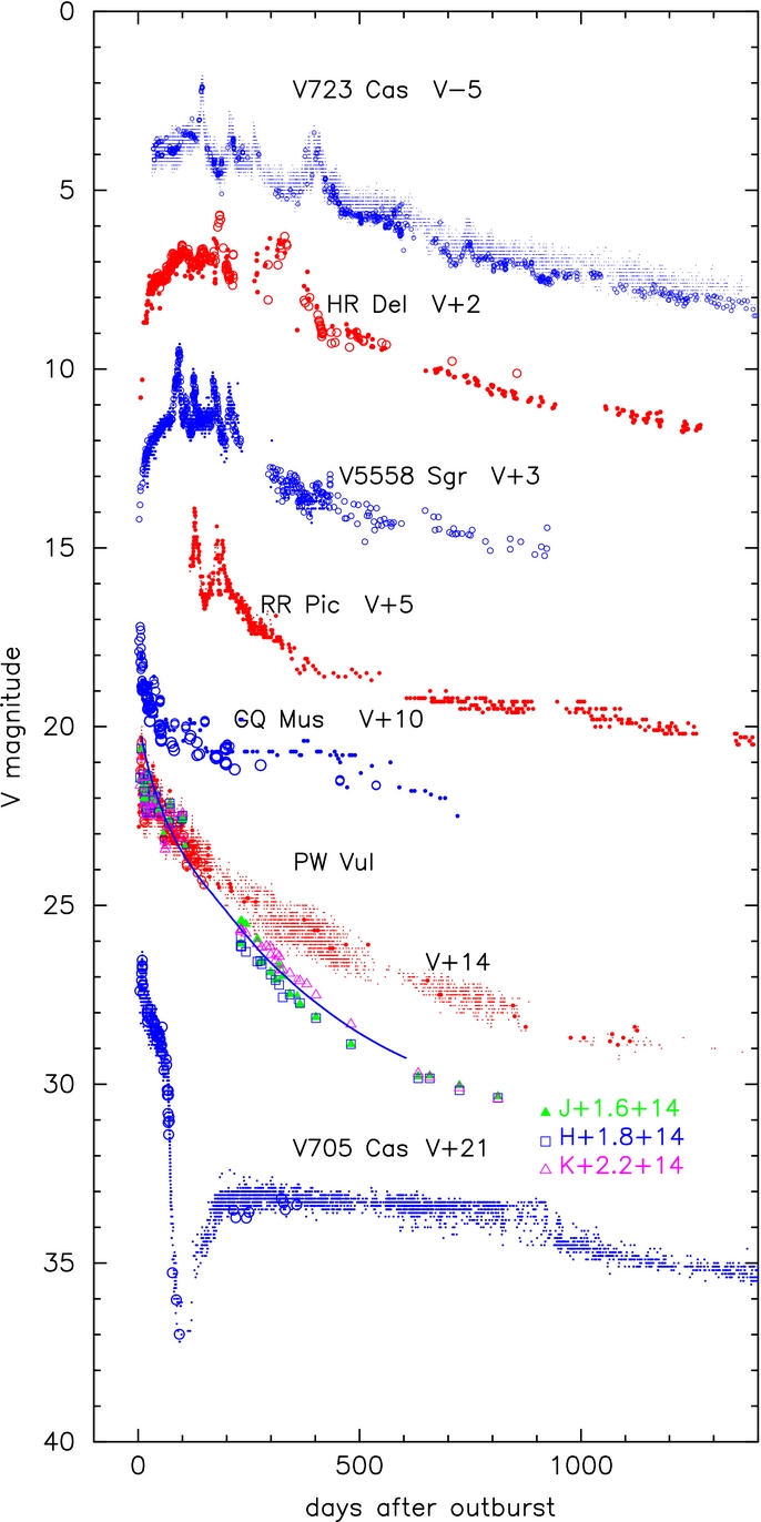
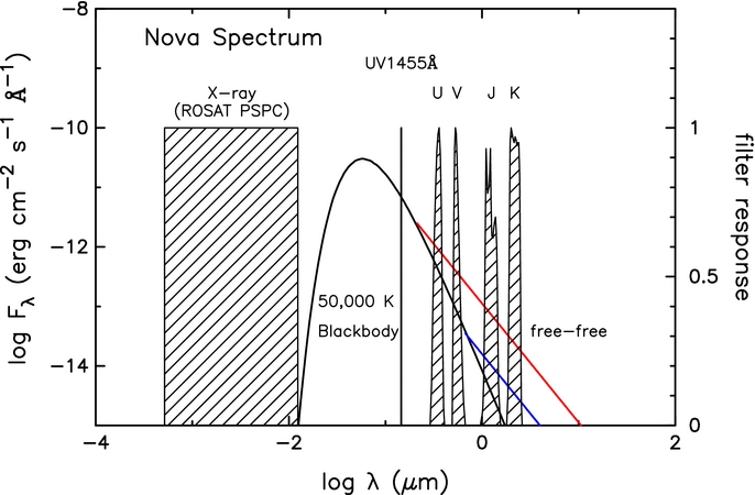
Figure 36. Maximum magnitude vs. rate of decline (MMRD) relation. Solid black line, i.e., Equation (A12): our model MMRD relation calibrated with PW Vul (large black open circle). Black dashed line: another model MMRD relation calibrated with V1668 Cyg (green filled square, Hachisu & Kato 2010), i.e., MV, max = 2.5log t3 − 11.6. Solid blue line labeled "MMRD1," i.e., Equation (A13): Kaler–Schmidt's law (Schmidt 1957). Solid magenta line labeled "MMRD2," i.e., Equation (A14): della Valle–Livio's law (della Valle & Livio 1995). Red filled star: the recurrent nova RS Oph as an example for a very high mass-accretion rate and very short timescale t3 (very small fs) (Hachisu & Kato 2010). Red open diamond: the 1 yr recurrence period M31 nova, M31N2008-12a, taken from Tang et al. (2014), i.e., Mg, max = −6.6 (maximum in the g band) and t3, g ≈ 4.2 days (measured in the g-band light curve). Red filled circles: individual novae taken from Table 5 of Downes & Duerbeck (2000). Large red filed circle: PW Vul taken from Table 5 of Downes & Duerbeck (2000). Large open black circle: PW Vul estimated from our model light curve of 0.83 M☉ WD. See text for more details.
Download figure:
Standard image High-resolution image
For comparison, two empirical MMRD relations are plotted in the same figure, i.e., Kaler–Schmidt's law (solid blue line labeled "MMRD1"; Schmidt 1957), i.e.,

and della Valle–Livio's law (solid magenta line labeled "MMRD2": della Valle & Livio 1995), i.e.,

where we used a relation of t2 ≈ 0.6 × t3 for the optical light curves that follow the universal decline law (Hachisu & Kato 2006).
Figure 36 also shows observational points for individual novae (red filled circles), taken from Table 5 of Downes & Duerbeck (2000). Note that we remeasured the t3 time of PW Vul along our model light curve, which resulted in t3 = 80 days and MV, max = −6.9, as shown by a large black open circle. This data point is to the left of Downes & Duerbeck's (2000) estimate (t3 = 126 day and MV, max = −6.7), denoted by a large red filled circle.
The scatter of the observed data with respect to the MMRD formulae in Figure 36 is generally large and larger than the observational errors. This strongly suggests that the scatter is due to the presence of a second parameter. Hachisu & Kato (2010) pointed out that the main parameter governing the MMRD relation is the WD mass (represented by the time-scaling factor fs in Figure 36), the second parameter being the initial envelope mass (or the mass-accretion rate of the WD). In turn, the initial envelope mass (ignition mass) depends on the mass-accretion rate to the WD (see, e.g., Figure 3 of Kato et al. 2014) such that the lower the mass-accretion rate, the larger the envelope mass. This simply means that for the same WD mass, novae are brighter/fainter for lower/higher mass-accretion rates. Hachisu & Kato (2010) clearly showed the dependence of maximum brightness on the initial envelope mass (see their Figures 8 and 15). We further show fainter examples of maximum brightness, RS Oph and M31N2008-12a, both of which are recurrent novae with ∼20 and ∼1 yr recurrence periods, respectively. We conclude that this second parameter, the initial envelope mass, can reasonably explain the scatter of individual novae from the empirical MMRD relations so far proposed (see Figure 15 of Hachisu & Kato 2010).
APPENDIX B: TIME-STRETCHING METHOD
The distance modulus of PW Vul can be estimated, in a very different way, from a resemblance between PW Vul and other optically well-observed novae. Hachisu & Kato (2006) found that nova light curves follow a universal decline law when free–free emission dominates the spectrum in optical and NIR regions. Using this property, Hachisu & Kato (2010) found that if two nova light curves overlap each other after one of the two is squeezed/stretched by a factor of fs (t' = t/fs) in the time direction, the brightnesses of the two novae obey the relation of

which is the same as Equation (A6). Using this property with calibrated nova light curves, we can estimate the absolute magnitude of a target nova. Figure 2 shows time-normalized light curves of PW Vul, V1668 Cyg, V1974 Cyg, and V533 Her against that of V1500 Cyg, similar to Figure 41 of Hachisu & Kato (2014), but we used the reanalyzed data. The V light curve and B−V and U−B color curves of PW Vul are well squeezed to match the other ones. Note that the dereddened (B − V)0 and (U − B)0 of each nova also follow a general course in the color–color diagram (i.e., overlap each other; see Hachisu & Kato 2014, for the general course of UBV color evolution of novae). These five novae obey the relations of

where ΔV is the difference of apparent brightness obtained in Figure 2 by which the V light curve of each nova is shifted up or down against that of V1500 Cyg. The time-scaling factors are also obtained in this figure as fs = 0.182 for PW Vul, fs = 0.44 for V1668 Cyg, fs = 0.42 for V1974 Cyg, and fs = 0.54 for V533 Her, each against that of V1500 Cyg. We obtained these stretching factors by shifting horizontally each light curve to overlap them. The apparent distance moduli of V1500 Cyg, V1668 Cyg, and V1974 Cyg were calibrated as (m − M)V, V1500 Cyg = 12.3, (m − M)V, V1668 Cyg = 14.25, and (m − M)V, V1974 Cyg = 12.2 in Hachisu & Kato (2014). These three are all consistent with each other. The distance modulus of V533 Her was also calculated to be (m − M)V, V533 Her = 10.8. Hachisu & Kato (2014) obtained the distance modulus of PW Vul based on this time-stretching method as (m − M)V = 13.0 ± 0.1, which is consistent with Equation (1). This is a strong support to our adopted values of E(B − V) = 0.55 and d = 1.8 kpc.