


ABSTRACT
We present a new chemical evolution model for dwarf spheroidal galaxies (dSphs) in the local universe. Our main aim is to explain both their observed star formation histories and metallicity distribution functions simultaneously. Applying our new model for the four local dSphs, that is, Fornax, Sculptor, Leo II, and Sextans, we find that our new model reproduces the observed chemical properties of the dSphs consistently. Our results show that the dSphs have evolved with both a low star formation efficiency and a large gas outflow efficiency compared with the Milky Way, as suggested by previous works. Comparing the observed [α/Fe]–[Fe/H] relation of the dSphs with the model predictions, we find that our model favors a longer onset time of Type Ia supernovae (i.e., 0.5 Gyr) than that suggested in previous studies (i.e., 0.1 Gyr). We discuss the origin of this discrepancy in detail.
Export citation and abstract BibTeX RIS
1. INTRODUCTION
In the standard hierarchical galaxy formation models, dwarf galaxies are the most numerous and elemental systems in the universe; larger galaxies are formed from smaller objects like dwarf galaxies through major and/or minor mergers (e.g., Kauffmann et al. 1993; Cole et al. 1994; Robertson et al. 2005). Thus, it is important to study these galaxies as the building blocks of normal bright galaxies to understand the formation and evolution of normal galaxies. In the Local Group, there are the following two types of dwarf galaxies (e.g., Mo et al. 2010): dwarf spheroidals (dSphs) and dwarf irregulars (dIrrs). While dIrrs are gas-rich systems and show current star formation activities, dSphs are gas-poor and consist of mainly old stellar systems.
Recent observations have unveiled the detailed star formation histories (SFHs) of dwarf galaxies in the local universe (Hernandez et al. 2000; Saviane et al. 2000; Carrera et al. 2002; Rizzi et al. 2003; Dolphin et al. 2005; Lee et al. 2009; Tolstoy et al. 2009; Weisz et al. 2011; de Boer et al. 2012a, 2012b), revealing a significant diversity among the SFHs of dwarf galaxies. Weisz et al. (2011) showed color–magnitude diagrams (CMDs) of 60 nearby dwarf galaxies within 4 Mpc from our Galaxy using the Hubble Space Telescope and estimated their SFHs through the CMDs. They found that the majority of dwarf galaxies exhibit a long duration of SFH, consisting of both a dominant ancient star formation (>10 Gyr ago) and a lower level of star formation at intermediate times (1–10 Gyr ago). They also found that the SFHs between dSphs and dIrrs are generally indistinguishable over most of the cosmic time. However, they pointed out that there is a clear difference between them in the most recent ∼1 Gyr, i.e., dSphs do not show much star formation activity in this epoch, but dIrrs do.
The SFHs of galaxies also affect their chemical abundance. The stellar chemical abundance in some dSphs has been observationally investigated by using the 8–10 m class large telescopes with high- and/or medium-resolution optical spectrographs (Shetrone et al. 2001, 2003; Tolstoy et al. 2003; Sadakane et al. 2004; Geisler et al. 2005; Bosler et al. 2007; Aoki et al. 2009; Cohen & Huang 2009, 2010; Kirby et al. 2010; Letarte et al. 2010; Tafelmeyer et al. 2010; Aden et al. 2011; Starkenburg et al. 2013). The derived chemical abundance indicates that dSphs have fewer metal-rich stars than the Milky Way (MW) disk; the average metallicity of stars in dSphs is ∼10–100 times lower than that of the MW disk stars. Moreover, their chemical abundance shows different trends from the MW halo, which suggests that dSphs have experienced different chemical evolution histories from that of the MW.
The chemical evolution histories of the dSphs have also been investigated theoretically based on the numerical models (Ikuta & Arimoto 2002; Carigi et al. 2002; Lanfranchi & Matteucci 2003, 2004; Fenner et al. 2006; Cescutti et al. 2008; Calura & Menci 2009; Kirby et al. 2011a; Tsujimoto 2011; Romano & Starkenburg 2013). These studies have revealed that both gas outflow and infall are important to reproduce the observed chemical abundance and/or the metallicity distribution functions (MDFs) of dwarf galaxies (Lanfranchi & Matteucci 2004; Kirby et al. 2011a, hereafter K11). For dSphs, a large gas outflow efficiency and lower star formation efficiency (SFE) than those of the MW have been predicted for their small metallicities; the outflow rate per star formation rate (SFR) and the SFE of the MW are ∼0.5 and ∼0.24 Gyr−1, respectively (Joung 2012; Kennicutt & Evans 2012).
Recently, Kirby et al. (2010) measured chemical abundances of 2961 stars in eight dSphs, which provided a large and homogeneously analyzed sample of stellar spectra in dSphs. In order to extract SFHs of the dSphs from their observed data, K11 constructed a detailed chemical evolution model including chemical yields from Type Ia and II supernovae (SNe Ia and SNe II, respectively) and from asymptotic giant branch (AGB) stars, as well as gas infall and outflow induced as an SN wind. The model simultaneously reproduced the observed trends of [Mg/Fe], [Si/Fe], and [Ca/Fe] ratios with [Fe/H], as well as MDFs in the dSphs. However, it should be emphasized that the duration timescales of their derived SFHs were only ∼1 Gyr (see Table 3 in K11), which are much shorter than those observationally estimated from the CMDs in dSphs (Dolphin 2002; Lee et al. 2009; de Boer et al. 2012a, 2012b). Moreover, although they stated that the derived star formation timescales were extremely sensitive to the minimum delay time of SN Ia, tdelay, min, they showed the resultant SFHs adopting two different values of tdelay, min only for one dSph among their eight dSphs in total (see Figure 10 in K11).
In this paper we construct a new analytic model of the chemical evolution of galaxies to reproduce both the observed SFHs and MDFs of dSphs, simultaneously. Our model explicitly utilizes the SFH derived from the observed CMD in dSphs as the most fundamental input quantity. Although this idea is similar to that proposed by Ikuta & Arimoto (2002) and Carigi et al. (2002), they compared their results only with the observed chemical abundance ratios of stars in dSphs. Since MDF is more sensitive to SFH than abundance ratio, we compare our model results with the observed MDFs in dSphs. While the abundance ratios are determined by the yields of chemically dominant stars at each epoch, MDF depends on both SFH and age–metallicity relation (AMR). Therefore, if we find a consistent solution for both the CMD and chemical property of a certain dSph, we obtain its MDF and AMR simultaneously from our chemical evolution model based on its observationally estimated SFH. We also compare our model results for the [Mg/Fe]–[Fe/H] relation to investigate the minimum delay time of the SN Ia; since the SN Ia explodes with a delay time and ejects large amounts of Fe relative to the SN II, the [Mg/Fe]–[Fe/H] relation suddenly changes when the SN Ia starts to explode.
The rest of this paper is organized as follows. The details of our chemical evolution model are described in Section 2. In Section 3, we present the results of our model in comparison with observations. After some discussions, including the comparison of our model results with those of K11 one in Section 4, the summary of this paper is given in Section 5.
2. THE CHEMICAL EVOLUTION MODEL CALCULATIONS
2.1. Basic Assumption and Formulation
Here we describe our new chemical evolution model to reproduce simultaneously both the observed SFHs and MDFs of the following four local dSphs: Fornax, Sculptor, Leo II, and Sextans. We adopt the following assumptions in our model, which are the same as those in K11, except items 2, 6, and 8.
- 1.The interstellar medium (ISM) of a dSph is treated as one zone, that is, we do not consider any spatial variations of gas density and metallicity in the ISM at any time.
- 2.The observed SFH derived from the analysis of the CMD is used in our model. Therefore, the SFR at time t, Ψ(t), is fixed to the observed one. Namely, our model is calculated along with the SFH.
- 3.
- 4.The interstellar gas can be expelled from a dSph (i.e., gas outflow) while supplied from its outside (i.e., gas infall), that is, the dSph in our model is not a closed box.
- 5.Gas outflow is assumed to be induced via a superwind (a collective effect of a large number of SNe), so that its rate is proportional to the total number of SNe Ia and II at each time. Metallicity of the outflow gas is assumed to be the same as that of the system at that time.
- 6.The number of SNe Ia is determined by the past SFH and the delay time distribution (DTD) function. The DTD function used in our model is the observationally derived one of Maoz et al. (2010). The minimum delay time of SNe Ia, tdelay, min, is adopted to be one of the model parameters.
- 7.The number of SNe II is determined by the past SFH and the stellar lifetime given by Timmes et al. (1995). We assume that stars with m ⩾ 10 M☉ explode as SNe II.
- 8.Gas infall rate is adjusted to reproduce the observed SFH. Since we assume that the SFR is fixed (item 2) and the gas mass of the ISM correlates with the SFR (item 3), the gas mass at time t, Mgas(t), is determined by the observed SFH. Moreover, the time derivative of the gas mass,
 , depends on the SFR, the ejected gas mass from evolved stars (i.e., AGBs and SNe Ia and II), the gas outflow via a superwind (item 5), and the gas infall. Therefore, in order to reproduce the gas mass, we set the gas infall rate as an adjustable amount (see Section 2.1.3). The metallicity of the infall gas is assumed to be primordial.
 - 9.The yield of SNe Ia and II is adopted from Iwamoto et al. (1999) and Nomoto et al. (2006), respectively. For the AGB yields, we adopt those of Karakas (2010). We assume that all stars with m < 10 M☉ evolve into AGBs after their lifetimes. All heavy elements are assumed to stay in gas phase during the entire time of calculation.
- 10.The initial mass function (IMF) used in our model, ϕ(m), is that derived by Kroupa et al. (1993) with a mass range of m = 0.08–100 M☉.

We calculate the chemical evolution for 119 elements and isotopes listed in Iwamoto et al. (1999), Nomoto et al. (2006), and Karakas (2010) under the assumptions listed above. The equations of the mass evolution and the chemical evolution for an element i at time t are represented by

and
where Mgas, i(t) is the gas-phase mass of an element i in the ISM at time t, Xi(t) is the gas-phase mass fraction for the element to the total mass of interstellar gas (Xi(t) ≡ Mgas, i(t)/Mgas(t) and ∑iXi(t) = 1), Ei(t) is the rate of gas mass for the element ejected from evolved stars to the ISM and E(t) is its total (E(t) = ∑iEi(t)), and  and
and  are its infall and outflow rates, respectively. We assume that both the initial abundance of the ISM and the infall gas are primordial (i.e., XH(t = 0) = Xin, H = 0.75 and XHe(t = 0) = Xin, He =0.25).
The ejected gas mass Ei(t) is given by the sum of three independent terms as follows:

where  ,
,  , and
, and  represent the rates of gas masses ejected from SNe Ia (Iwamoto et al. 1999), SNe II (Nomoto et al. 2006), and AGBs (Karakas 2010), respectively. The term
  can be written by using the number of SNe II and Ia,
  and
and  , respectively, as

where

and
Here the outflow coefficient Aout (M☉ SN−1) controls the outflow gas mass per unit SN. For the DTD function, we adopt the following, which are observationally estimated by Maoz et al. (2010):
where tdelay indicates an elapsed time since the progenitor star of an SN Ia is formed. The variable τ(m) in Equation (6) is the stellar lifetime of the star with mass of m.
The interval of each time step in our calculation is Δt = 25 Myr.3 The calculation is terminated when the SFR reaches zero or a certain condition, which is described in detail in Section 2.2, is satisfied.
The assumptions adopted in our model listed above are the same as K11 except the assumptions for the SFH (item 2), minimum delay time of SNe Ia (item 6), and gas infall rate (item 8). It should be stated that, while the stellar lifetime adopted in our model (Timmes et al. 1995) is also different from that in K11 (i.e., Padovani & Matteucci 1993; Kodama 1997), the difference is found to not affect the resultant chemical evolution. In the following subsections we describe these major differences in the model assumptions between K11 and ours.
2.1.1. Star Formation History and Gas Mass
In our model, we use the SFHs estimated from the photometric observations for our sample dSphs (i.e., Fornax, Sculptor, Leo II, and Sextans) as the most fundamental inputs. On the other hand, in K11, SFH is not an input quantity but one of the output quantities, which is determined to reproduce the observed data of the MDF and abundance ratios for each one of their samples of the local dSphs, including our sample dSphs. In Figure 1 we show the SFHs of our sample dSphs derived in the literature (Fornax: de Boer et al. 2012b; Sculptor: de Boer et al. 2012a; Leo II: Dolphin 2002; Sextans: Lee et al. 2009). It should be emphasized that the observed SFHs have much longer timescales of about 8–13 Gyr than the timescales of the SFHs derived in K11 of ∼0.8–1.3 Gyr.

Figure 1. SFHs of our sample dSphs. The histograms with error bars are observational estimates for the SFHs derived from the CMDs (Fornax: de Boer et al. 2012b; Sculptor: de Boer et al. 2012a; Leo II: Dolphin 2002; Sextans: Lee et al. 2009). The error bars indicate the uncertainties caused by the so-called CMD model, by using which the SFH can be estimated from the CMD. The red dotted lines are the SFHs used in our model calculations obtained through a linear interpolation of the observed SFHs.
Download figure:
Standard image High-resolution imageIt should be noted that the SFHs of both Leo II and Sextans start from 15 Gyr ago, which is longer than the age of the universe derived from the current cosmology (Komatsu et al. 2009). As for this discrepancy, Lee et al. (2009) mentioned that the current level of discrepancy is within the range of various plausible adjustments for the stellar models. However, for safety, we have compared the best-fit parameters, whose details are described in Section 2.2, of Sextans for the SFHs starting from 15 Gyr ago and 14 Gyr ago, and we have confirmed that there is no difference. Namely, the discrepancy is not critical to the chemical evolution of the dSphs. Therefore, we have decided to let it stand.
For each dSph in our sample, we derive its SFR at each time step via linear interpolation of the discrete data points of its observed SFH. Note that the observational estimates for SFH used here contain uncertainties, as shown in Figure 1, originating from the model that decodes the SFH of a dSph from its CMD, the so-called CMD model. However, we do not incorporate such uncertainties in the process to obtain Ψ(t) via linear interpolation; therefore, SFH used in our calculation does not include uncertainties of the CMD model.
We then calculate the gas-phase mass in the ISM of the dSph at time t, Mgas(t), as
where A* and α are the same parameters as in the K11 model. While K11 defined the unit of A* as 106 M☉ Gyr−1, we set A* as the nondimensional parameter. This formulation explains the relation between total mass of interstellar gas Mgas(t) and Ψ(t) (i.e.,  , the generalization of a Kennicutt–Schmidt law). While K11 treated α as one of their model parameters and found that its best-fit value varies among their sample of dSphs (see Table 2 in K11), we fix it to unity in our model for simplicity. When α = 1, the parameter A* takes the same value of the SFE (i.e., =Ψ(t)/Mgas(t)) in units of Gyr−1. We investigate the effect of using a fixed α on other model parameters through a comparison with the K11 model results in Section 4.3.
2.1.2. Type Ia Supernovae
We assume that SNe Ia explode according to the past SFH and the adopted DTD function with the parameter that represents the minimum delay time for SNe Ia, tdelay, min. These assumptions are the same as that of K11, except for the value of tdelay, min. K11 adopted a single value of tdelay, min = 0.1 Gyr, while they concluded that the derived star formation timescale is extremely sensitive to tdelay, min; larger tdelay, min results in a longer star formation timescale. Since the star formation timescale in our model is much longer than that derived in K11, we adopt the following two values for the minimum delay time for SNe Ia: tdelay, min = 0.1 Gyr and 0.5 Gyr.
2.1.3. Gas Infall
While the gas infall rate at a certain time t,  , is represented by
  in K11, where τin is one of their model parameters, it is determined in our model so that Equation (1) is satisfied at any time in the calculation. This difference comes from the different assumption for the SFH described in Section 2.1.1. In our model, once the SFH of a certain dSph is given, Mgas(t) at any t is determined via Equation (8) with an adopted parameter of A*, and hence
  is also fixed. Moreover,
  and
and  in Equation (3) and
  in Equation (4) are completely determined because the stellar lifetime and both yields of SNe II and AGBs used in our model are all fixed. The terms
  and
and  in these equations also depend on SFH, as well as one of the parameters in our model, tdelay, min. Therefore, all variables in Equation (1) except for
  are determined for a given SFH and set of parameters in our model, that is, A*, Aout, and tdelay, min. In a more qualitative sense, our prescription for gas infall rate means that, while the SN blows out part of the gas from the ISM of the dSph, star formation can take place according to the observed SFH so that the primordial gas flows into the system at the same time.
Nevertheless, the gas infall rate determined in this way would be negative when the time derivative of gas mass,  , is negative and the outflow rate,
  , is low. Such a negative infall rate acts effectively as outflow. However, this implies that the system would blow out not only enriched gas by SNe but also extra primordial gas simultaneously. This is contrary to one of the assumptions in our model, that the system is chemically homogeneous. To avoid such physically unlike situations, we artificially add an extra outflow rate
  to Equation (1) so that the resulting infall rate becomes zero during such a situation. Therefore, the gas infall rate is determined via the following equation rather than Equation (1):

Since the metallicity of outflow gas is assumed to be the same as that of the system at that time in our model, introducing such extra outflow gas solves the physically unlike situation described above. Although the introduction of such an extra outflow rate is completely artificial, it should be stated that external processes to remove gas from dSphs such as tidal stripping can act as this extra outflow rate. This is because the outflow rate in our model is simply assumed to be linearly proportional to the SN rates as represented by Equation (4).
As a consequence of introducing the extra outflow rate, the net outflow rate ( ) is not proportional to the SN rate transiently when
  is not equal to zero. In order to evaluate the importance of the extra outflow rate quantitatively, we define Fex as the total mass ratio of the extra outflow to the net outflow in the entire SFH of a dSph, which can be represented by
where tfin is the time at which our calculation ends (see Section 2.2 for its detailed definition). If Fex = 0, there is no extra outflow gas required for the dSph during the model calculation. If 0 < Fex ⩽ 1, the model needs extra gas outflow during the model calculation.
Although this modification is artificial, the derived best-fit model parameters are consistent within their 1σ uncertainties whether or not this modification is adopted for our sample. The detailed definition of the best-fit model and 1σ uncertainties are described in the next section and Section 3.1, respectively.
2.2. Determination of the Best-fit Model
In our model, there are three free parameters to fit the observed MDF as follows: SFE (A*), outflow coefficient (Aout), and minimum delay time for SNe Ia (tdelay, min). The best-fit parameters are determined through the following two steps. First, for each dSph in our sample, we calculate the evolution history of iron abundance, ζFe(t) ≡ [Fe/H](t), using the model provided with its SFH. When we calculate the abundance, we adopt the solar composition of Sneden et al. (1992) for Fe: 12 + log (nFe/nH)☉ = 7.52. The parameter ranges explored are A* = 10−3–10 and Aout = 102–105 M☉ SN−1, equally spaced in logarithmic scale with a step of 0.01 dex. For tdelay, min, we examine the following two cases: tdelay, min = 0.1 Gyr and 0.5 Gyr. Therefore, the total number of the parameter sets is 120,000 for each tdelay, min. Then, the best-fit model for each tdelay, min is individually determined by using a maximum likelihood estimation, which maximizes the following likelihood L:
where ζFe, j = [Fe/H]j and ΔζFe, j = Δ[Fe/H]j are the observed iron abundance and its uncertainty of the jth star in the dSph, respectively. The variable  is evaluated in our model according to the SFH of the dSph, where M* is the stellar mass of the dSph at present and
  is the mass of the stars that are newly formed in the dSph at time t and survive until the present. We note that, since both M* and
  are completely determined from the input SFH, the factor
  does not depend on our model parameters and simply acts as a weight in the likelihood calculation. Therefore, the best-fit parameters can be different among our sample dSphs.
For the observed iron abundance of our sample dSphs, we use the data provided in Kirby et al. (2010), in which the iron abundance [Fe/H] of nearly 3000 stars in eight dSphs, including our sample dSphs, is spectroscopically measured by using Fe i absorption lines. It should be noted that these sample stars are different from those used to derive the SFHs. In general, the area in a dSph spectroscopically observed is different from that photometrically observed, as shown in Table 1; the area observed spectroscopically is typically smaller than that observed photometrically and concentrates on the center of each dSph. However, since we assume that the dSph in our model is chemically homogeneous at any time, we simply assume that the stars sampled in the photometric and spectroscopic observations both well represent the entire population in the dSph. We will discuss the influences of such differences in the observed area on the resultant chemical evolution histories in Section 4.2.
Table 1. Half-light Radii and Observed Area of the dSphs
| dSph | Half-light Radius | Observed Area | Reference | |
|---|---|---|---|---|
| Spectroscopy | Photometry | |||
| Fornax | ∼16' | ∼20' × 20' | ∼1 5 × 10 5 × 10 |
1, 2, 3 |
| Sculptor | ∼11' | ∼20' × 20' | ∼17 × 17 |
1, 2, 4 |
| Leo II | ∼2 6 6 |
∼20' × 15' | ∼13 × 13 |
1, 2, 5 |
| Sextans | ∼28' | ∼35' × 20' | ∼42' × 28' | 1, 2, 6 |
References. (1) McConnachie 2012; (2) Kirby et al. 2010; (3) de Boer et al. 2012b; (4) de Boer et al. 2012a; (5) Mighell & Rich 1996; (6) Lee et al. 2009.
Download table as: ASCIITypeset image
In our calculation for chemical evolution, the metallicity of the system can change violently with time. Specifically, such a violent change of metallicity happens just before the end of the SFH, where the mass of interstellar gas becomes very low and comparable with that of outflowing gas. In this condition, a small amount of yield is sufficient to change the metallicity of the interstellar gas, which is supplied via infall of gas with primordial composition. Therefore, we set the following two criteria to determine the condition for the violent change of metallicity:
or

where Δt is the interval of individual time steps (=25 Myr). If either of these criteria is satisfied, we terminate the calculation and set tfin at the time, which is used to calculate the likelihood via Equation (11).
3. RESULTS
3.1. The Best-fit Models
We first compare the MDFs and chemical abundance ratios of the best-fit models for our sample dSphs with those of the observed data in Figure 2. For the observed data in both the left and right panels of Figure 2, we plot only the stars with the uncertainties in both metallicity and abundance ratio less than or equal to 0.3 dex, while we do not adopt any cutoff for the uncertainties during the likelihood calculation. We also show the abundance ratios of some of the other elements calculated in our model, that is, [Si/Fe], [Ca/Fe], and [Ti/Fe], in Appendix B.
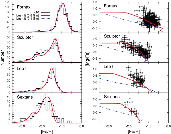
Figure 2. MDFs and [Mg/Fe]–[Fe/H] diagrams. The histograms (left) and data points with error bars (right) show the observed MDFs and [Mg/Fe] ratios, respectively, taken from Kirby et al. (2010). Only observed data with uncertainties less than or equal to 0.3 dex are shown. The blue dotted and red solid curves are the results of our best-fit models with tdelay, min = 0.1 Gyr and 0.5 Gyr, respectively.
Download figure:
Standard image High-resolution imageIt is found that the resultant MDFs of the best-fit models reasonably reproduce the observed data. Specifically, the peak metallicities at which the observed MDFs have the largest frequencies of stars are well fitted by the best-fit models for all of our sample dSphs. Moreover, the tails in the observed MDFs elongated into metal-poor sides from the peak metallicities, which are different among the dSphs, are also reproduced by the best-fit models. On the other hand, although the observed MDF for Sextans shows a broader metal-rich tail with Δ[Fe/H] ∼ 1 dex than those for the other three dSphs of Δ[Fe/H] ∼ 0.5 dex, the model MDFs have similar metal-rich tails with Δ[Fe/H] ∼ 0.5 dex in all dSphs despite the difference in their SFHs. It is also found that there are bumps in the model MDFs with tdelay, min = 0.5 Gyr at [Fe/H] ∼ −2.3 in Sculptor and [Fe/H] ∼ −2.5 in Sextans, while such bumps are not evident in the observed MDFs.
The peak metallicities in the MDFs are found to correlate with Aout; the model MDF with smaller Aout has a peak at higher metallicity. It is also found that the metal-poor tail is related to SFH; the dSph forming stars more intensively in the past tends to have a more elongated tail. On the other hand, the significance of the bump seen in the metal-poor tail is found to correlate with the model parameters A* and tdelay, min, as well as the SFH. We discuss the effects of our model parameters of Aout, A*, and tdelay, min on the MDF in detail in Section 4.1.
3.2. The Best-fit Model Parameters and Their Uncertainties
The best-fit model parameters with their 1σ uncertainties are listed in Table 2 and shown in Figure 3. It is important to note again that these uncertainties do not include the uncertainties in SFHs shown in Figure 1, as described in Section 2.1.1. If the uncertainties in the SFH are included, the derived uncertainties of the best-fit model parameters will be larger.
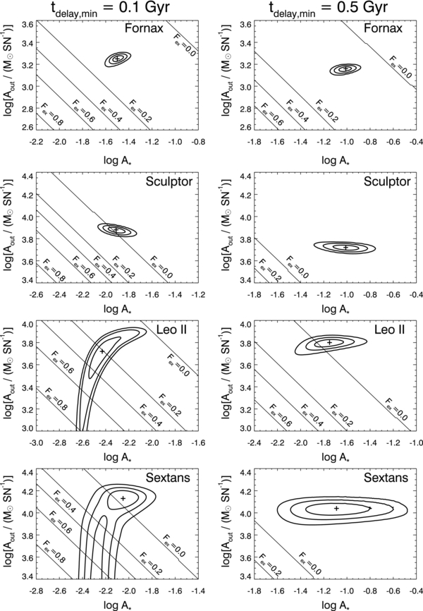
Figure 3. Confidence levels for the model parameters, Aout and A*, with tdelay, min = 0.1 Gyr (left) and 0.5 Gyr (right). Plus signs represent the best-fit model parameters, and thick solid contours in each panel indicate 1σ, 2σ, and 3σ confidence levels. Thin solid curves show the contours of Fex corresponding to 0.0, 0.2, 0.4, 0.6, and 0.8 as indicated in the key.
Download figure:
Standard image High-resolution imageTable 2. The Best-fit Model Parameters with Their 1σ Uncertainties, the Maximum Likelihoods, and the Fractions of Extra Outflow Gas Mass
| dSph | tdelay, min = 0.1 Gyr | tdelay, min = 0.5 Gyr | ||||||
|---|---|---|---|---|---|---|---|---|
| log A* | log [Aout/(M☉ SN−1)] | −log Lmax | Fex (%) | log A* | log [Aout/(M☉ SN−1)] | −log Lmax | Fex (%) | |
| Fornax |  |
 |
175 | 4.4 |  |
 |
170 | 0.54 |
| Sculptor |  |
 |
252 | 0.00 |  |
 |
243 | 0.00 |
| Leo II |  |
 |
110 | 21 |  |
 |
113 | 0.00 |
| Sextans |  |
 |
111 | 0.00 |  |
 |
108 | 0.00 |
Download table as: ASCIITypeset image
As shown in Figure 3, both of the model parameters A* and Aout are well determined using the observed MDFs, except those with tdelay, min = 0.1 Gyr for Leo II and Sextans, whose contours are apparently elongated. Such elongated contours of constant confidence levels are attributed to large Fex. Large Fex implies that the extra gas outflow contributes significantly to the outflow from the system rather than the superwind; therefore, the model results depend weakly on Aout.
For each dSph, the likelihoods of the best-fit models with tdelay, min = 0.1 Gyr and 0.5 Gyr are found to be similar to each other, as shown in Table 2. This result implies that the best-fit value of tdelay, min for a certain dSph cannot be evaluated by analyzing its MDF alone, while Aout and A* can be determined by the metallicity at which the MDF has a peak and the significance of the metal-poor tail in the MDF, respectively. However, this difficulty for tdelay, min can be solved through a comparison of the model with observed data in the [Mg/Fe]–[Fe/H] plane, as shown in the right panels of Figure 2. It is clearly shown that, for all of the sample dSphs, the evolution tracks of the model with tdelay, min = 0.5 Gyr in the plane provide better fits to the observed data than those with tdelay, min = 0.1 Gyr. This difference of the evolution track in the [Mg/Fe]–[Fe/H] plane originates from the difference between the SN Ia and SN II yields. Since the SN Ia yields have a smaller abundance ratio of [α/Fe] than the SN II yields, [α/Fe] of the system starts to decrease when SN Ia starts to explode, that is, when the time of tdelay, min is elapsed since the onset of star formation.
Through this comparison for our sample dSphs, it is found that tdelay, min = 0.1 Gyr is too short to fit the observed distribution of the stars in the [Mg/Fe]–[Fe/H] plane. However, this result is clearly against the observational estimates for the minimum delay time of SNe Ia, which provides tdelay, min ≲ 0.1 Gyr almost certainly (Totani et al. 2008; Maoz et al. 2010). This discrepancy between our model prediction and the observational estimate to tdelay, min is discussed in Section 4.4.
3.3. Time Evolution of Mass and Gas Flow of the Best-fit Models
We show the time evolution of stellar mass M*(t) and total mass of interstellar gas Mgas(t), as well as the total mass of the system M*(t) + Mgas(t) calculated from the best-fit models for our sample dSphs in Figure 4. Note that since the observed SFH is adopted as the input in our model, the time evolution of stellar mass is completely independent of model parameters; therefore, both of the shapes and absolute values of M*(t) for a dSph calculated from the best-fit models with tdelay, min = 0.1 Gyr and 0.5 Gyr are identical to each other. Moreover, since gas mass at a given time is assumed to be linearly proportional to the SFR at the time, Ψ(t), according to Equation (8), the time evolution of gas mass for a certain dSph has exactly the same shape as that of its SFR by definition. Therefore, the shape of Mgas(t) is independent of the model parameters, as shown in Figure 4. However, the ratio of Mgas(t)/Ψ(t) is controlled by one of the model parameters A* in the sense that smaller A* results in larger gas mass for a given SFR. For the dSphs for which A* of the best-fit models are very low (i.e., log A* ≲ −2), that is, Sculptor, Leo II, and Sextans with tdelay, min = 0.1 Gyr, gas mass dominates the total mass of the dSph in almost the entire time during the calculation.

Figure 4. Time evolution of various masses calculated from the best-fit models for our sample dSphs. Left and right panels show the best-fit models with tdelay, min = 0.1 Gyr and 0.5 Gyr, respectively. The black solid and blue dotted curves represent the stellar masses and interstellar gas masses, respectively, while the red dot-dashed curves show their total masses.
Download figure:
Standard image High-resolution imageThe time evolution of the outflow and infall rates of the best-fit models are shown in Figure 5. It is found that, while the outflow rate evolves smoothly, the shape of the time evolution of the infall rate is like a step function, except for Leo II. This step-function-like shape of the infall rate originates from the prescription for the infall rate in our model; that is, the infall rate is adjusted to satisfy the condition of Equation (9) for a given SFH. Thus, the infall rate can suddenly change at the time when the slope of SFR changes (see Figure 1). In this sense, such step-function-like evolution of the infall rate is a rather artificial result caused by using the observationally estimated SFH with coarse time resolution. On the other hand, since the outflow rate is determined by the number of SNe Ia and SNe II as described in Equation (4) and hence the SFR, the time evolution of the outflow rate looks similar to the SFH and smoother than the infall rate.
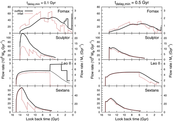
Figure 5. Same as Figure 4, but for the time evolution of the outflow and infall rates. The vertical axis on the right side indicates the outflow and infall rates per present stellar mass of each dSph. The present stellar masses of Fornax, Sculptor, Leo II, and Sextans are M* = 2.3 × 10⁷, 4.9 × 10⁶, 3.7 × 10⁵, and 9.6 × 10⁵ M☉, respectively, which are estimated by their SFHs. The black solid and red dotted curves represent the outflow and infall rates, respectively. For the outflow rates, the thin and thick black curves present the original outflow rates of  , which are evaluated via Equation (4), and the net outflow rates of
  , respectively.
Download figure:
Standard image High-resolution imageFor the best-fit models for Leo II with tdelay, min = 0.1 Gyr and for Fornax with both tdelay, min, bumps are also seen in the outflow rates at the late stages of evolution, that is, the look-back time of ∼1–6 Gyr for Leo II and ∼2 Gyr and ∼0 Gyr for Fornax. These bumps originate from the contributions of the extra outflow gas masses to avoid the negative infall rate explained in Section 2.1.3. The fractions of extra outflow gas masses Fex of these models are Fex = 4.4%, 0.54%, and 21% for the best-fit models for Fornax with tdelay, min = 0.1Gyr and 0.5 Gyr and for Leo II with tdelay, min = 0.1Gyr, respectively. This artificial prescription for the extra outflow tends to appear in the late stages of evolution, where the increasing rate of metallicity of the system is smaller than that in the early stage, as shown in Figure 6. Therefore, the effect of this extra gas outflow on the MDF is small.

Figure 6. AMRs calculated from the best-fit models for our sample dSphs. The best-fit models with tdelay, min = 0.1 Gyr and 0.5 Gyr are shown as blue dotted and red solid curves, respectively.
Download figure:
Standard image High-resolution imageThe gas flow rates of the models with lower A* are larger since the gas masses are larger. Total outflow gas masses are ∼10–100 times larger than the present stellar masses. It is worth noting that the outflow and infall rates are comparable. This result implies that a large amount of infalling gas, which is comparable to outflowing gas associated with star formation, is inevitably required to reproduce both low average metallicity and relatively long SFH of dSph simultaneously. Specifically, in order to explain the observed low metallicities of dSphs, a large amount of metals is required to be blown away by superwinds. However, since a large amount of gas outflow terminates the star formation in dSphs rapidly, a comparable gas infall is necessary to reproduce relatively long SFHs estimated observationally for dSphs. We will provide a discussion for the chemical evolution of dSphs and comparison with the results of previous works in Section 4.5.
4. DISCUSSION
4.1. The Dependence of Chemical Evolution on the Model Parameters
In Section 3.1, we show that the observed MDFs of our sample dSphs are reasonably reproduced by our best-fit models. Here we investigate the detailed dependence of MDF on our model parameters of A*, Aout, and tdelay, min. Considering that the MDF is roughly determined by the SFH and the AMR as
and that the SFH is fixed in our model, the MDF will depend only on the AMR. Therefore, through investigating the effects of the model parameters of A*, Aout, and tdelay, min on the AMR, which are shown in Figure 7, we can examine their effects on the MDF. Note that while the illustrated models in Figure 7 are only the cases for Sculptor, the AMRs for the other dSphs show a similar dependence on the model parameters.
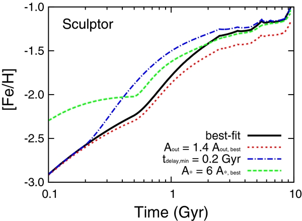
Figure 7. Comparison of the AMRs calculated from the models with various sets of the model parameters of Aout, tdelay, min, and A*, including the best-fit model parameters for Sculptor. While the black curve represents the AMR of the best-fit model with tdelay, min = 0.5 Gyr, the other curves show the AMRs of the models where one of the parameters for the best-fit model is changed. For the red dotted, blue dot-dashed, and green dashed curves, the parameters changed from the best-fit one are Aout, tdelay, min, and A*, respectively, as indicated in the key.
Download figure:
Standard image High-resolution imageAs shown in Figure 7, compared with the AMR of the best-fit model with tdelay, min = 0.5 Gyr (black solid curve), the AMR of the model with larger Aout (red dotted curve) results in a slower metal evolution, and its deviation from the best-fit model increases monotonically with time. This is because, for a given SFR, a larger Aout leads to a larger amount of metal elements expelled from the system as a more intense outflow, resulting in a smaller growth rate of metallicity. Since the deviation from the best-fit model seems to be evident throughout the late stages of chemical evolution, Aout affects the mean metallicity of the system; larger Aout leads to smaller mean metallicity. In fact, the best-fit models for our sample dSphs show this trend (see Table 2 and Figure 2). In other words, our model predicts that the observed low metallicities of dSphs are the consequence of intense gas outflows accompanied by a large amount of metal.
On the other hand, the effect of changing tdelay, min from the value in the best-fit model of tdelay, min = 0.5 Gyr into 0.2 Gyr appears in the early phase of chemical evolution, as shown by the blue dot-dashed curve in Figure 7. Since the SN Ia supplies much abundant Fe to the ISM compared to SNe II and AGBs, metallicity of the system increases rapidly just after the SN Ia starts to explode, that is, the minimum delay time tdelay, min is elapsed since the onset of star formation. Therefore, the AMRs with different tdelay, min are clearly different in the early stages of chemical evolution. However, the growth rate of metallicity decreases with time, and hence the difference between the models with different tdelay, min becomes negligible in the late phases of chemical evolution. Therefore, the effect of tdelay, min is important in the early phase of chemical evolution, in particular around t ∼ tdelay, min.
The effect of changing A* appears also in the early phase of chemical evolution, as shown by the green dashed curve in Figure 7. Since a higher A* means that the system has smaller gas mass for a given SFR according to Equation (8), the interstellar gas of the system is easily enriched by the yields from the evolved stars, which are fixed from the past SFH. Therefore, the model with a higher A* results in a more rapid chemical enrichment in the early phase. However, the growth rate of metallicity decreases with time similar to the model with changing tdelay, min. As a result, changing A* affects the metal evolution mainly in the early phase.
Specifically, a lower A* results in a larger number of metal-poor stars, producing a broader metal-poor tail in the MDF. In other words, the dSph whose MDF has a broad metal-poor tail is expected to prefer a low A*. However, the best-fit parameters of A* show no relation with the broadness of the metal-poor tails in the MDFs against the expectation from our model; while Sculptor has a broader metal-poor tail than Fornax and Leo II, the best-fit parameter of A* for Sculptor is similar to that for Fornax and larger than that for Leo II (see Table 2). This contradiction comes from the fact that the effect of A* on the metal-poor tail in MDF is not primary but secondary. The broadness of the metal-poor tail in MDF is primarily determined by the SFH, or more specifically, the fraction of the stars formed in the early phase of chemical evolution. As shown in Figure 1, the fraction of the stars formed in the early phase is large in Sculptor but small in Fornax and Leo II. When we calculate the chemical evolution for Fornax, Sculptor, and Leo II with the same A*, the metal-poor tails in the resultant MDFs would be broader in Sculptor and narrower in Fornax and Leo II. In other words, the value of A* is determined not only by the shape of the metal-poor tail in MDF but also by the shape of the SFH.
Moreover, the similarity between the effects of changing tdelay, min and A* on the AMR leads to the degeneracy between these parameters in our chemical evolution model. As shown in Figure 2 and Table 2, the observed MDFs can be reproduced regardless of tdelay, min since the model MDF with short tdelay, min and low A* is similar to the model with long tdelay, min and high A*. This degeneracy can be resolved by comparing the model results with the observed [Mg/Fe]–[Fe/H] diagrams simultaneously since different tdelay, min results in different abundance ratios of α elements as described in Section 3.2. Therefore, both the observed MDF and abundance ratio are required to determine tdelay, min and A* accurately.
In summary, it is difficult to understand the chemical evolution of dSphs only by analyzing the MDF and abundance ratio. It is important to examine the MDF, abundance ratio, and SFH simultaneously for investigating the chemical evolution of dSphs.
4.2. The Effects of the Difference in Observed Area on the SFH and MDF
As already stated in Section 2.2, the observed area for a dSph in which its MDF is evaluated is typically different from that to obtain SFH. In our model, the difference in the observed area is completely neglected since dSph is assumed to be chemically homogeneous. However, photometric observations for dSphs have reported that some dSphs have a radial gradient with age and metallicity; young stars are more concentrated than old stars, and metal-rich stars are more concentrated than metal-poor stars (de Boer et al. 2012a, 2012b; Lee et al. 2009). Therefore, the dSphs are not chemically homogeneous, and the difference in the observed area for the SFH and MDF may affect our results.
In order to investigate the effect of this difference on the model results, we calculate the chemical evolution for Fornax and Sculptor by using their SFHs and MDFs evaluated from the stars in the same area, that is, the central region (rell < 02) obtained by de Boer et al. (2012a, 2012b), where rell is the elliptical radius of the dSphs used in de Boer et al. (2012a, 2012b). As shown in Figures 8 and 9, while the number of metal-poor stars in the observed MDFs is slightly underestimated, our model can reproduce the observed MDFs for Fornax and Sculptor with almost the same parameters, except Aout for Fornax.4 A large amount of extra gas outflow (i.e., Fex > 0.8) in the past several gigayears.

Figure 8. Top: SFH of the central region (rell < 02) of Fornax obtained by de Boer et al. (2012b) and the SFH used in our model calculation represented by the thick histogram and red solid curve, respectively. For reference, the SFHs shown in Figure 1 are also presented as the thin histogram and blue dotted curve. Middle: observed and best-fit model MDFs for the SFH of the central region of Fornax, shown as histograms and red solid curves, respectively. Note that the observed MDF shown as the histogram is the same as that shown in the top left panel of Figure 2. The best-fit models with the parameters listed in Table 2 are also plotted by blue dotted curves, for reference. Bottom: same as Figure 5, but for the time evolution of the outflow and infall rates in the best-fit models for the SFH and MDF in the central region of Fornax. In the middle and bottom, left and right panels show the best-fit models with tdelay, min = 0.1 and 0.5 Gyr, respectively.
Download figure:
Standard image High-resolution image
Figure 9. Same as Figure 8, but for Sculptor.
Download figure:
Standard image High-resolution imageWe also calculate the chemical evolution for Fornax by using the MDF evaluated from the 562 stars in a wide area (∼10 × 15) of Fornax (Battaglia et al. 2006), which is comparable to the observed area for SFH by de Boer et al. (2012b). Although the observed MDF in the wide area shows a larger number of metal-poor stars than the MDF shown in Figure 2, our model cannot reproduce it as shown in Figure 10. Moreover, a significant amount of extra outflow (i.e., Fex > 0.8) is required for the past ∼8 Gyr, as shown in the bottom panels of Figure 10.
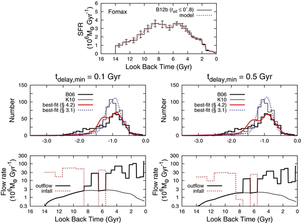
Figure 10. Same as Figure 8, but for the observed data and best-fit models for the SFH and MDF in a wide area of Fornax. The MDF of a wide area obtained by Battaglia et al. (2006) is shown as a thick histogram in the middle panels, while the observed SFH and MDF shown as a thin histogram in the top and middle panels are the same as those plotted in the top panel of Figure 1 and top left panel of Figure 2, respectively.
Download figure:
Standard image High-resolution imageThe results of the above comparison indicate that our model for chemical evolution cannot explain both the SFH and MDF simultaneously in the central and/or the whole regions of Fornax. This difficulty can be relaxed if the SFE (i.e., A* with the units of Gyr−1) is adopted to be time variant, which is suggested from observational studies (e.g., Combes et al. 2013). Since the SFE controls the growth rate of metallicity in the early phase as described in Section 4.1, the model with a time-variable SFE can form a larger number of metal-poor stars.
A multizone model is also expected to resolve the difficulty in our model for the number of metal-poor stars. Some studies presented a signature of multicomponent structure in dSphs. It is reasonable that the metal-poor population in a dSph has experienced different chemical evolution from the metal-rich population. Hence, it is important to gather many observational results of dSphs and construct a more realistic multizone chemical evolution model.
4.3. Comparison of the Best-fit Parameters with Those of K11
As described in Section 2.1, our model is basically the same as that of K11. The best-fit parameters in K11 for our sample dSphs are listed in Table 3. Since the unit of A* in our model is different from that in the K11 model ( ), we show converted values of A* from
  in Table 3 by
  ). Then we can directly compare the best-fit parameters derived from the K11 model with ours.
Table 3. The Best-fit Model Parameters with tdelay, min = 0.1 Gyr of K11, Our Model, and Comparison Models for Our Sample dSphs
| dSph | Parameter | K11 | Comparison Model | Our Model | |||
|---|---|---|---|---|---|---|---|
| Case 1 | Case 2 | Case 3 | Case 4 | ||||
| α | 0.98 |
0.98 (fixed) | 0.98 (fixed) | 1.0 (fixed) | 1.0 (fixed) | 1.0 (fixed) | |
| Fornax | log A* | 0.70 |
1.14 |
1.14 |
1.14 |
−1.30 |
−1.50 |
| log [Aout/(M☉ SN−1)] | 3.18 |
3.18 (fixed) | 3.16 |
3.16 |
3.32 |
3.25 |
|
| α | 0.83 |
0.83 (fixed) | 0.83 (fixed) | 1.0 (fixed) | 1.0 (fixed) | 1.0 (fixed) | |
| Sculptor | log A* | −0.33 |
−0.32 |
−0.30 |
−0.41 |
−2.21 |
−1.91 |
| log [Aout/(M☉ SN−1)] | 3.73 |
3.73 (fixed) | 3.70 |
3.68 |
2.95 |
3.88 |
|
| α | 0.66 |
0.66 (fixed) | 0.66 (fixed) | 1.0 (fixed) | 1.0 (fixed) | 1.0 (fixed) | |
| Leo II | log A* | −0.37 |
−0.26 |
−0.25 |
−0.48 |
−2.08 |
−2.43 |
| log [Aout/(M☉ SN−1)] | 3.82 |
3.82 (fixed) | 3.80 |
3.78 |
3.91 |
3.72 |
|
| α | 0.50 |
0.50 (fixed) | 0.50 (fixed) | 1.0 (fixed) | 1.0 (fixed) | 1.0 (fixed) | |
| Sextans | log A* | −0.28 |
−0.29 |
−0.30 |
−0.74 |
−2.47 |
−2.05 |
| log [Aout/(M☉ SN−1)] | 3.98 |
3.98 (fixed) | 3.91 |
3.91 |
3.97 |
4.13 |
|
Download table as: ASCIITypeset image
It is found that while the values of Aout in K11 are similar to those in our best-fit models, A* of our best-fit models with tdelay, min = 0.1 Gyr are much smaller than those of K11. To investigate the origin of this difference, we explore the best-fit models for the following four cases: (Case 1) the model with the fixed SFH, α, and Aout that are the same as those in K11 and with only one adjustable parameter of A*; (Case 2) the model with the same SFH and α as those in K11 and with adjustable parameters of A* and Aout; (Case 3) the model with the same SFH as that in K11 and with three adjustable parameters α (fixed to unity), A*, and Aout; and (Case 4) the model with the same shape of the SFH as K11, but its timescale is extended to fit the timescale of our SFH. The resultant best-fit parameters for the four cases are listed in Table 3.
In the Case 1 model, in which only one parameter of A* can be used to fit the observed MDF, the best-fit values of A* for our sample dSphs are similar to those in K11, as shown in Table 3. This result indicates that, if the same SFH and parameters are adopted, the resultant MDFs from the K11 and our models are similar to each other. Although the best-fit A* is significantly different from that in K11 for Fornax, the discrepancy of A* between the K11 and our model is attributed to the different prescription for gas infall rate. Since the infall rate at t = 0 is adopted to be exactly equal to zero in the K11 model, high A* results in rapid consumption of interstellar gas, terminating star formation in a very short timescale. Since the best-fit SFH of Fornax in the K11 model decreases rapidly in the first short epoch (i.e., ≲ 0.1 Gyr), A* is considered to be a maximum in their model. On the other hand, since the infall rate in our model is adjusted to keep the interstellar gas mass satisfying the required condition of Equation (8) for a given SFR, A* can be explored to fit the observed MDF.
The best-fit parameters of A* and Aout in the Case 2 model are similar to those in the Case 1 model. In the Case 3 model, in which α is changed from the best-fit values in K11 to unity, the best-fit parameters of Aout are similar to those of Case 2, but those of A* become lower. In other words, A* and α are degenerate.
The best-fit values of A* change dramatically in the Case 4 model, in which the SFH timescales are modified into those used in our model of ∼10 Gyr; A* decreases more than one order of magnitude, while Aout is similar to that in the Case 3 model, except for Sculptor.5 The significant decrease of A* can be interpreted as follows. In order to reproduce a given MDF, a longer star formation timescale requires a slower chemical evolution, that is, a lower value of A*. As a consequence, the Case 4 model provides a set of the best-fit parameters that is quite similar to that of our model, as shown in Table 3. The tiny differences between the two sets of the best-fit parameters are caused by differences in the shapes of SFH.
Therefore, we can conclude that the difference in the best-fit parameters of A* between the K11 and our model originates from the difference in the star formation timescale for dSph. Furthermore, although Fenner et al. (2006) made their model fitting for the observed chemical abundance of Sculptor and found that the [α/Fe] is degenerated between the duration of the SFH and the SN feedback, our model fitting for the observed MDFs shows no degeneracy between the duration of the SFHs and the Mout (see Cases 3 and 4 in Table 3). We emphasize that, since the parameters in the chemical evolution model are sensitive not only to the MDF but also to the SFH, it is important to fit the MDF and SFH simultaneously in order to investigate the chemical evolution of dSphs.
4.4. The Discrepancy of the Minimum Delay Time for SNe Ia between Our Model Results and Observations
In Section 3.2, we show that our model disfavors the minimum delay time of tdelay, min ∼ 0.1 Gyr since it is too short to reproduce the observed distribution of the stars in our sample dSphs in the [Mg/Fe]–[Fe/H] plane (see right panels of Figure 2). This is against the recent observational and/or theoretical estimates for tdelay, min, which show that tdelay, min ≲ 0.1 Gyr (e.g., Totani et al. 2008; Cooper et al. 2009; Maoz & Mannucci 2012; Kistler et al. 2013). While the K11 model with tdelay, min = 0.1 Gyr successfully reproduces the observed distributions in the [Mg/Fe]–[Fe/H] plane, it results in too short star formation timescales compared to those estimated observationally for the dSphs. Therefore, to explain both the SFH and the chemical abundance of dwarf galaxies simultaneously, a longer tdelay, min than the observationally favorable value of ∼0.1 Gyr seems to be required inevitably. What are the origins of this discrepancy in tdelay, min between our chemical evolution model and the observational and theoretical estimates?
One of the origins of this discrepancy can be the dependence of SN Ia rate on metallicity. Taking account of the suggestion from some theoretical works that the SN Ia rate in metal-poor galaxies is smaller compared to metal-rich galaxies (Kobayashi et al. 1998; Kobayashi & Nomoto 2009; Meng et al. 2011), we consider that the effect of the SN Ia yields on the abundance ratio of [Mg/Fe] will be smaller in the early metal-poor stages of chemical evolution than in the late metal-rich stages. Incorporating such a metal-dependent SN Ia rate into our model with short tdelay, min will result in the same abundance ratios as the model with long tdelay, min because, in addition to the onset time of the first SN Ia, extra metal enrichment time is required. Therefore, the discrepancy can be relaxed if such a metallicity dependence of the SN Ia rate is taken into account. However, the opposite dependence on metallicity has also been suggested (e.g., Cooper et al. 2009; Kistler et al. 2013). Therefore, it is still unclear how tdelay, min depends on the metallicity of the system.
Another possible origin of this discrepancy can be the one-zone approximation adopted in our model; it is an apparently oversimplified approximation for the dSphs because the age and metallicity gradients have been observed in them as described in Section 4.2. If we adopt a multizone approximation instead of the one-zone one, the discrepancy can be relaxed. While the one-zone model assumes that the system is chemically homogeneous, multizone models probably can describe these complicated structures. In the multizone approximation, zones can have different SFHs from each other, and the ejecta of SNe II and SNe Ia can flow from one zone to another. If a zone has a short (<0.1 Gyr) star formation event and its star formation ceases before the SN Ia ejecta from nearby zones flows into the zone, the chemical abundance of stars formed there reflects only the SN II ejecta. In other words, the chemical evolution model with a multizone approximation can increase the metallicity of the stars without the effect of SNe Ia.
The assumption of the time-independent IMF is also one of the origins of the discrepancy, since some theoretical works predicted a different IMF when the metallicity of the system is low. Tumlinson (2006) suggested that low-mass star formation was inhibited when the metallicity of the system was below a critical metallicity (i.e., Zcr ≲ 10−4 Z☉). If the system forms only massive stars when the metallicity of the ISM is low, the ISM is chemically enriched without the contribution of SNe Ia. Therefore, the metallicity-dependent IMF can relax the discrepancy about tdelay, min.
Some previous studies argue that dSphs have a bottom-heavy IMF and/or lack very massive (⩾25 M☉) stars (Tsujimoto 2011; Li et al. 2013; Weidner et al. 2013). Li et al. (2013) analyzed the chemical abundance of the stars in Fornax dSph and concluded that a bottom-heavy IMF is necessary to explain the low [α/Fe]. However, the low [α/Fe] is also explained by the large contribution of the SNe Ia (Ikuta & Arimoto 2002; Lanfranchi & Matteucci 2004; Tolstoy et al. 2009; K11), and a bottom-heavy IMF cannot explain the high [α/Fe] (e.g., [Mg/Fe] > 0.5), such as observed in our samples. To confirm the effect of the bottom-heavy IMF on our model results, we calculate the chemical evolution of the samples by changing the stellar mass upper limit from 100 M☉ to 25 M☉. However, we have found that the model MDFs have no changes and the model [Mg/Fe] decrease with decreasing mass upper limit at the same [Fe/H] about 0.2 dex. Therefore, the model with a bottom-heavy IMF and tdelay, min = 0.1 Gyr results in worse fitting to the observed data.
4.5. The Chemical Evolution Histories of dSphs Indicated by Our Best-fit Models
4.5.1. The Star Formation Efficiencies of Dwarf Galaxies
As shown in Table 2, the best-fit values of the SFE (A*) for our sample dSphs are 10−2.4 to 10−1.0 Gyr−1. Here we compare these model results with the observational estimates for the SFEs of dwarf galaxies. Note that the SFE derived in our model is constant during the entire history of the galaxy, while the SFE estimated from a star-forming dwarf galaxy reveals its current value.
Figure 11 shows such a comparison of the SFE as a function of the stellar mass between our model results and the observational estimates. In this plot, the observational estimates for the SFEs of the star-forming dwarf galaxies are shown instead of dSphs since the star-forming dwarf galaxies have enough interstellar gas and SFR to be detected by observations, which are inevitable to evaluate current SFE. From 48 Im galaxies whose H i gas masses and Hα luminosities are obtained by McCall et al. (2012) and Kennicutt et al. (2008), respectively, the mean SFE is evaluated as 〈log [SFE/Gyr−1]〉 = −1.4 ± 0.7, which is consistent with our best-fit SFEs. The mean SFEs of Im and Sm galaxies in Hunter & Elmegreen (2004) are 〈log [SFE/Gyr−1]〉 = −1.4 ± 0.5 and −1.1 ± 0.5, respectively, which are also comparable to those of our best-fit models. The mean SFE of blue compact dwarfs (BCDs), 〈log [SFE/Gyr−1]〉 = −0.6 ± 0.5, is found to be higher by almost 1 mag than our best-fit SFEs.

Figure 11. Comparison of the model results with observed data of star-forming dwarf galaxies in the SFE–stellar mass plane. The model results are plotted as filled symbols, while the observed data are plotted as open symbols. The filled circles and diamonds with error bars are the results of the best-fit models with tdelay, min = 0.1 and 0.5 Gyr, respectively. The open circles are the data of Im galaxies estimated from gas and stellar masses in McCall et al. (2012) and Hα luminosities in Kennicutt et al. (2008). The open squares, triangles, and diamonds are the data of Im, BCD, and Sm galaxies, respectively, estimated from gas masses and Hα luminosities in Hunter & Elmegreen (2004) and stellar masses derived from Hunter & Elmegreen (2006) and Bell & de Jong (2001).
Download figure:
Standard image High-resolution imageThe result of this comparison of the SFE is consistent with the observed result that the mean SFHs of the different morphological types of dwarf galaxies, including dSph and dIrr, are indistinguishable from each other over most of cosmic time (Weisz et al. 2011). Therefore, the dIrrs may experience the same chemical evolution histories as the dSphs essentially. It is indicated that if dIrrs exhaust all their interstellar gas, they can evolve into dSphs (Kormendy 1985; Peeples et al. 2008; Zahid et al. 2012).
4.5.2. The Gas Outflow from dSphs
As described in Section 3.3, our best-fit parameter values of Aout for our sample dSphs are found to be significantly large; the total masses of outflow gas are 10–100 times larger than the final stellar masses of the dSphs. The best-fit parameter values of Aout themselves and/or the result of a significant amount of outflow gas are consistent with the results from other analytic models for chemical evolution (Lanfranchi & Matteucci 2003, 2004, 2007, 2010; Lanfranchi et al. 2006a, 2006b, 2008; K11). This amount of outflow gas mass is consistent with the physically possible maximum value,  , estimated from the following simple consideration: 100% of the SN energy is converted into the kinetic energy of outflow gas with a typical escape velocity of ∼25 km s−1 (Sculptor; Sánchez-Salcedo & Hernandez 2007), resulting in
  or
or  . Nevertheless, this amount of outflow gas mass significantly depends on the assumption regarding the metallicity of outflow gas. The low metallicity of the dSphs is achieved not by the amount of gas outflow but by the amount of ejected metals.
In our best-fit models with tdelay, min = 0.1 Gyr (0.5 Gyr), the mass fractions of Fe ejected from the system to the totally synthesized Fe in the system are evaluated as 95% (91%), 99% (98%), 99% (98%), and 99% (99%) for Fornax, Sculptor, Leo II, and Sextans, respectively; that is, more than 90% of Fe is lost from all of our sample dSphs as outflow powered by superwinds, whose amount is consistent with those of Kirby et al. (2011b). This high ejected mass fraction of Fe is inevitably required to reproduce the observed low metallicities of the dSphs. In our model, 100% of the SN ejecta is assumed to be mixed instantaneously within the ISM at once before gas outflow occurs; the SN ejecta are diluted with the entire interstellar gas, and the metallicity of outflow gas becomes significantly smaller than that of the SN yields.
High-resolution chemo-dynamical simulations suggest that only a low fraction of SN ejecta stays in the region where stars form (Marcolini et al. 2006; Revaz & Jablonka 2012). For example, according to the results from Revaz & Jablonka (2012) that the SN feedback efficiency of 0.03–0.05 is sufficient to reproduce the properties of the dSphs, the mass fraction of the SN ejecta mixing with the ISM is estimated to be only ∼5%. In this estimation, the total mass of outflow gas results in only ∼0.1% of the final stellar masses for all of our sample dSphs. Therefore, the total mass of outflow gas can vary about five orders of magnitude according to the assumption of the metallicity of outflow gas. This result indicates that the ejected metal mass fraction of >90% is more essential in the chemical evolution history of dSphs than the total mass of outflow gas.
In order to constrain the total mass of outflow gas, it is important to evaluate what fraction of SN ejecta is directly expelled from the system. However, it is strikingly difficult to observe the outflow from dSphs since they have almost no gas at present. In contrast, the outflowing gas has been observed in dIrrs (Heckman et al. 2001; Martin et al. 2002; van Eymeren et al. 2009a, 2009b, 2010). For the dIrr starburst galaxy NGC 1569, Martin et al. (2002) estimated the metal content of outflow gas by using Chandra and concluded that the outflow transports most of the metals synthesized by current starbursts. If the dIrrs are considered to be the progenitors of the dSphs as described in Section 4.5.1, which still have plentiful gas and show ongoing star formation activity, these observational results imply that a significant fraction of SN ejecta is also directly expelled from dSphs. Therefore, the total masses of outflow gas of dSphs seem to be smaller than their current stellar masses.
5. SUMMARY
We have constructed a new analytic model for the chemical evolution to reproduce both the observed SFH and MDF of a dSph, simultaneously. While the prescriptions and assumptions in our model are similar to those adopted in K11, there are critical differences between them, as described in Section 2.1: the assumptions for the SFH, the minimum delay time for SNe Ia, and infalling gas. With this new model, we have performed model calculations for Fornax, Sculptor, Leo II, and Sextans, and we compare the derived MDFs with observed MDFs. Our results and conclusions are summarized as follows.
- 1.It is demonstrated that our new models can reproduce the observed MDFs of the dSphs with various metallicity. We have found that their MDFs are characterized by two parameters: the SFE (A*) and the gas outflow efficiency (Aout).
- 2.It is shown that the likelihoods of the best-fit models for the dSphs do not depend on the minimum delay time of SNe Ia (tdelay, min). This means that any constraints are not obtained by analyzing both the MDFs and the SFHs. We have found that the best-fit models with tdelay, min = 0.1 Gyr underestimate the observed [Mg/Fe] of the dSphs, while previous studies have suggested tdelay, min ≃ 0.1 Gyr. In our models, tdelay, min is required to be much longer than 0.1 Gyr to explain the observed SFHs, MDFs, and [Mg/Fe] simultaneously.
- 3.The derived SFEs of the dSphs are lower than that estimated observationally for the MW (∼0.24 Gyr−1) and those obtained theoretically for the dSphs by K11. These low SFEs lead to a small growth rate of metallicity and broad metal-poor tail in the MDF. The best-fit values of SFE are similar to those evaluated observationally for dIrrs with both rich gas and star formation activity. This is consistent with the observations of dwarf galaxies that the mean SFHs of the dSphs and dIrrs are indistinguishable from each other over most of cosmic time.
- 4.The derived Aout (the outflow gas mass per unit SN) are similar to those obtained theoretically for the dSphs by K11, and the outflow rate per SFR is larger than that estimated observationally for the MW (∼0.5). The large amount of gas outflow leads to a large amount of metal outflow and lower mean metallicity of the dSph. Our model predicts that the dSphs have lost more than 90% of iron synthesized in the systems; this is consistent with observational results that there is outflowing gas in some dIrrs like NGC 1569.
- 5.The derived gas infall rates are comparable to the derived gas outflow rates. Since the dSphs have low metallicities and relatively long SFHs, our model needs a large amount of metal outflows and a comparable amount of gas infalls to maintain the star formations as observed.
We are grateful to M. Chiba, K. Hayashi, D. Toyouchi, T. Otsuka, and T. Obata for insightful discussions and comments. We thank the referee for useful comments and suggestions. This work was financially supported in part by the Japan Society for the Promotion of Science (No. 23244031 (Y.T.)).
APPENDIX A: THE EFFECT OF THE DIFFERENT SIZE OF TIME STEP ON OUR MODEL RESULTS
We adopted a time step of 25 Myr in our calculations (Section 2.1). This step is much longer than that of K11 (ΔtK11 = 1 Myr). In this section we examine whether the time step affects the results or not.
For the four dSphs, we evaluate the best-fit parameters for time steps of Δt = 50, 20, 15, 10, 5, and 1 Myr for the parameter sets that sufficiently cover the areas of 1σ confidence level shown in Figure 3. As a result, it is confirmed that the 1σ confidence regions for Δt = 25 Myr include all the best-fit parameter sets for Δt = 1–50 Myr for all the sample dSphs with tdelay, min = 0.5 and 0.1 Gyr. In Figure 12 we show the result for Sculptor with tdelay, min = 0.5 Gyr as an example. The best-fit parameter set only slightly changes by changing the time step as shown in the left panel of Figure 12.
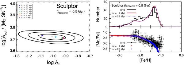
Figure 12. Left: best-fit parameters with various sizes of time step and the confidence levels for the model of Sculptor with tdelay, min = 0.5 Gyr. The black plus sign and the contours are exactly the same as those in Figure 3, that is, the best-fit parameter with Δt = 25 Myr and the 1σ, 2σ, and 3σ confidence levels, respectively. The best-fit parameters with Δt = 50, 20, 15, 10, 5, and 1 Myr are plotted as a blue asterisk, cyan diamond, green cross, orange triangle, red square, and blue plus sign, respectively. Right: MDFs and the [Mg/Fe]–[Fe/H] relations of Sculptor. The histogram and the data points with error bars are exactly the same as those in Figure 2, that is, the observed MDF and observed chemical abundance of stars in Sculptor, respectively. The red solid curve and blue dotted curve are the model MDFs, which are calculated by using the best-fit parameter set of Sculptor with tdelay, min = 0.5 Gyr as listed in Table 2, with time steps of Δt = 1 and 25 Myr, respectively. Red plus signs and blue crosses are also the model calculated by the same parameter set with Δt = 1 and 25 Myr, respectively; they are plotted at each time step.
Download figure:
Standard image High-resolution imageThe difference in the time step affects the chemical abundance of the ISM mainly at an early phase. In the right panel of Figure 12 we show the calculated MDF and the [Mg/Fe]–[Fe/H] relation for the best-fit models of Sculptor (tdelay, min = 0.5 Gyr) with Δt = 25 and 1 Myr. Note that the calculated [Mg/Fe]–[Fe/H] relation of each time step is shown by symbols. There is no significant difference between the model MDFs for Δt = 1 Myr and Δt = 25 Myr. At the early phase (i.e., [Fe/H] < −2.5), the values of [Mg/Fe] for Δt = 1 Myr are slightly larger than those for Δt = 25 Myr. Since the more massive stars have the shorter lifetimes, the chemical abundance of the ISM at the early phase depends on the yields of massive stars. In the first time step of calculations, stars with mass of m ⩾ 10 M☉ die within 25 Myr, while those with m ⩾ 100 M☉ die within 1 Myr. In other words, the model with Δt = 25 Myr cannot resolve the yields of stars with m ⩾ 10 M☉. However, the difference of this effect is small and negligible as metallicity increases. Therefore, the effect of the different time step on our model results is negligible.
APPENDIX B: THE ABUNDANCE RATIOS OF [Si/Fe], [Ca/Fe], AND [Ti/Fe]
Here we present the evolution of Si, Ca, and Ti, which are also shown in K11. As shown in Figure 13, the best-fit models with tdelay, min = 0.5 Gyr result in better fits to the observed data of [Si/Fe] and [Ca/Fe] provided in Kirby et al. (2010) than those with tdelay, min = 0.1 Gyr. This result is consistent with the result described in Section 3.2 and shown in the right panel of Figure 2, that is, tdelay, min = 0.1 Gyr is too short to reproduce the observed data of the dSphs.
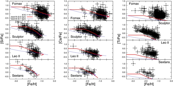
Figure 13. Chemical abundance ratios of [Si/Fe] (left panels), [Ca/Fe] (middle panels), and [Ti/Fe] (right panels). The data points with error bars are taken from Kirby et al. (2010). Same as the right panel of Figure 2, only observed data with uncertainties less than or equal to 0.3 dex are shown. The blue dotted and red solid curves are the results of our best-fit models with tdelay, min = 0.1 and 0.5 Gyr, respectively.
Download figure:
Standard image High-resolution imageOn the other hand, the best-fit models with both tdelay, min = 0.1 and 0.5 Gyr underpredict the observed data of [Ti/Fe], as shown in the right panel of Figure 13. Such underprediction is also seen in K11, and they ignored the model result for Ti since they consider that the yield for [Ti/Fe] is inaccurate. Therefore, this underprediction is simply because the SN II yield for [Ti/Fe] used in our model (Nomoto et al. 2006) is not high enough to reproduce the observed data.
Footnotes
- 3
- 4
The best-fit parameters of A* with tdelay, min = 0.1 Gyr (0.5 Gyr) for Fornax and Sculptor are
and , respectively. The best-fit parameters of Aout with tdelay, min = 0.1 Gyr (0.5 Gyr) for Sculptor are . On the other hand, since Fex of the best-fit models for Fornax are large, the best-fit parameters of Aout are not determined well. The 3σ upper limit of Aout is log [Aout/(M☉ SN−1)] = 3.02 (2.73) with tdelay, min = 0.1 Gyr (0.5 Gyr). - 5
The best-fit value of Aout for Sculptor in the Case 4 model has a large uncertainty because of a large Fex.

![$\log {[A_\mathrm{out} / (M_{\odot }\, \mathrm{SN}^{-1})]} = 3.86^{+0.03}_{-0.04}$](https://content.cld.iop.org/journals/0004-637X/799/2/230/revision1/apj506793ieqn51.gif)
