


ABSTRACT
Bright single pulses of many radio pulsars show rapid intensity fluctuations (called microstructure) when observed with time resolutions of tens of microseconds. Here, we report an analysis of Arecibo 59.5 μs resolution polarimetric observations of 11 P-band and 32 L-band pulsars with periods ranging from 150 ms to 3.7 s. These higher-frequency observations form the most reliable basis for detailed microstructure studies. Close inspection of individual pulses reveals that most pulses exhibit quasi-periodicities with a well-defined periodicity timescale ( ). While we find some pulses with deeply modulating microstructure, most pulses show low-amplitude modulations on top of broad smooth subpulse features, thereby making it difficult to infer periodicities. We have developed a method for such low-amplitude fluctuations wherein a smooth subpulse envelope is subtracted from each de-noised subpulse; the fluctuating portion of each subpulse is then used to estimate
  via autocorrelation analysis. We find that the microstructure timescale
  is common across all Stokes parameters of polarized pulsar signals. Moreover, no clear signature of curvature radiation in vacuum in highly resolved microstructures was found. Our analysis further shows strong correlation between
  and the pulsar period P. We discuss implications of this result in terms of a coherent radiation model wherein radio emission arises due to formation and acceleration of electron–positron pairs in an inner vacuum gap over magnetic polar cap, and a subpulse corresponds to a series of non-stationary sparking discharges. We argue that in this model,
  reflects the temporal modulation of non-stationary plasma flow.
Export citation and abstract BibTeX RIS
1. INTRODUCTION
Soon after the discovery of pulsars, Craft et al. (1968) noticed sub-millisecond (i.e., hundreds of microseconds) intensity structures in single pulses of PSR B0950+08. Subsequently, several high-time-resolution studies revealed rapid intensity variations superposed on the subpulses of several other pulsars. This phenomenon, usually known as pulsar microstructure, is currently thought to be associated closely with mechanisms of magnetospheric radio emission. Observationally, microstructures are found to occur simultaneously over a wide band (e.g., Rickett et al. 1975) and in pulsars with rotation periods down to 89 ms (Kramer et al. 2002), providing strong empirical evidence in favor of magnetospheric emission. The high brightness temperatures observed in pulsars rule out any thermal plasma processes and indicate that the underlying mechanism must be a coherent plasma process. However, a coherent radiation mechanism that provides a physical interpretation of microstructure behavior is yet to be identified.
Broadly, two appealing scenarios have been considered to explain microstructure emission, commonly known as angular beaming or temporal modulation. The angular beaming scheme is a geometrical phenomenon wherein intensity fluctuations result from an angular radiation pattern (mimicking microstructure width and periodicity) in the transverse direction. As the pulsar rotates, an observer then samples this emission structure. On the other hand, the temporal modulation scheme entails intensity fluctuation of propagating waves in the magnetosphere that finally reach the observer.
The existing microstructure studies fall into two broad categories: studies with very high time resolution (∼100 ns) that are needed to study narrow microstructures, and those with a coarser resolution (≳10 μs) that are useful for exploring the properties of broad microstructures. Among the former is the well-known detection of ultrafast 2 ns temporal structures in the Crab pulsar (Hankins et al. 2003; see also Jessner et al. 2010). Intensity fluctuations with timescales as small as 2.5 μs have also been reported in PSR B1133+16 by Bartel & Hankins (1982), and Popov et al. (2002) find micropulses with widths between 2 and 7 μs in pulsars B0950+08, B1133+16, and B1929+10. Most of the other well-known microstructure studies were geared to study the broad microstructures. These have shown that subpulses often show quasiperiodic intensity variations with periods of hundreds of microseconds (e.g., Hankins 1971; Boriakoff 1976; Soglasnov et al. 1981, 1983; Cordes et al. 1990). Cordes (1979) and Kramer et al. (2002) further show that the measured temporal width ( ) of a micropulse is related linearly to the rotation period P approximately as
  and
and  , respectively. Polarized microstructure has been investigated for a few pulsars (Ferguson & Seiradakis1978; Cordes 1979), and only for the Vela pulsar B0833-45 does some quantitative description exist (Kramer et al.2002). Further observations, analyses, and phenomenological assessments are needed to establish how microstructure is connected physically with the mechanisms of pulsar emission.
One of the difficulties in using the existing microstructure studies to amalgamate with pulsar emission theories is that they represent different resolutions, frequencies of observation, and analysis methods. Hence, in the remainder of our work, our main effort is to (1) carry out a systematic, single-frequency, single-instrument (Arecibo) study of the properties of broad polarized microstructure; and (2) study the physical implications of the microstructure characteristics in the context of currently favored coherent radio emission theories.
2. OBSERVATIONS
High-time-resolution single-pulse polarimetric observations were carried out using the Arecibo telescope for 32 pulsars in the frequency range of about 1.2–1.6 GHz (L-band) and 11 pulsars at around 327 MHz (P-band). For these observations, we used the Observatory's Mock spectrometers in the "single-pixel" polarimetry mode (see http://naic.edu/~astro/mock.shtml). These Fourier-transform-based instruments are capable of sampling at a ∼59.5 μs rate and producing Stokes spectra in a filterbank format. The details of the observations are given in Table 1. This moderate time resolution was chosen as suitable for both investigating broad microstructure and maximizing the number of objects that could be so observed. In the remainder of this paper, we will use the word "microstructure" to imply broad microstructure unless specified otherwise. Heretofore, only some 14 well-known bright pulsars have been subjected to microstructure studies (see Table 2 of Kramer et al. 2002 and the Vela pulsar), out of which 11 are in the Arecibo declination range. Our sample included 10 of these previously studied objects (except PSR B0540+23) at L band, as well as 22 others that are now accessible owing to both the Gregorian feed system and capacious Mock back-ends. At P band, there is an overlap with six pulsars; however, for most pulsars at this frequency (apart from B1929+10), either the dispersion or the scattering timescale is comparable with the sampling rate and hence they are not suitable for microstructure study. Nonetheless, given the novelty of this 59.5 μs polarimetry with excellent signal-to-noise ratio (S/N), we do display their properties in the online supplementary material. The high-time-resolution average polarization profiles of 24 pulsars at L band that were eventually used for microstructure study (see Section 3) are shown in Appendix
Table 1. Observational Parameters
| PSR | Band | MJD | Ch.BW (GHz)/ | Length | RM | DM | %L | %V |
|---|---|---|---|---|---|---|---|---|
| Name | (MHz) | Nchan | res (°)/μs | rad m−2 | pc/cc | |||
| B0301+19 | 337.668 | 55283 | 0.085/256 | 616/0.015/59.52 | −8.3 | 15.74 | 43 | 17 |
| B0525+21 | 351.764 | 56572 | 0.085/256 | 616/0.015/59.52 | −39.6 | 50.94 | 24 | −1.9 |
| J0546+2441 | 351.764 | 56573 | 0.024/1024 | 843/0.021/166.67 | −19.6 | 73.81 | 6 | −3.2 |
| B1919+21 | 352.806 | 55320 | 0.112/512 | 1139/0.016/62.5 | −16.5 | 12.46 | 14 | 8 |
| B1929+10 | 337.668 | 55320 | 0.085/256 | 4639/0.094/59.52 | −5.6 | 3.18 | 88 | −3.6 |
| B1944+17 | 352.806 | 55320 | 0.112/512 | 2269/0.051/62.5 | −28.0 | 16.22 | 6 | −6.6 |
| B2016+28 | 337.668 | 55320 | 0.085/256 | 953/0.038/59.52 | −34.6 | 14.17 | 23 | −0.7 |
| B2020+28 | 337.668 | 55320 | 0.085/256 | 4211/0.062/59.52 | −74.7 | 24.64 | 44 | 0.5 |
| B2044+15 | 337.668 | 55320 | 0.085/256 | 960/0.019/59.52 | −100.0 | 39.84 | 36 | −10.3 |
| B2110+27 | 337.668 | 55320 | 0.085/256 | 1265/0.018/59.52 | −37.0 | 25.11 | 4 | −3.3 |
| B2315+21 | 352.806 | 55275 | 0.112/512 | 275/0.015/59.52 | −35.8 | 20.91 | 32 | 3 |
| B0301+19 | 1220.668 | 55425 | 0.085/1024 | 1202/0.015/59.52 | −8.3 | 15.74 | 36 | 8.8 |
| B0525+21 | 1220.668 | 55522 | 0.085/1024 | 640/0.006/59.52 | −39.6 | 50.94 | 45 | −13.7 |
| J0546+2441 | 1220.544 | 56572 | 0.085/1024 | 421/0.007/59.52 | −19.2 | 73.81 | 35 | −13 |
| B0656+14 | 1220.668 | 55522 | 0.085/1024 | 1558/0.055/59.52 | −23.5 | 13.997 | 91 | −19.7 |
| B0751+32 | 1220.668 | 55522 | 0.085/1024 | 1944/0.014/59.52 | −7.0 | 39.949 | 29 | −26 |
| B0823+26 | 1220.668 | 55522 | 0.085/1024 | 1130/0.040/59.52 | 5.9 | 19.454 | 19 | 0 |
| B0834+06 | 1220.668 | 55522 | 0.085/1024 | 1006/0.017/59.52 | 23.6 | 12.889 | 15 | −4.5 |
| B0919+06 | 1220.668 | 55522 | 0.085/1024 | 1045/0.049/59.52 | 29.2 | 27.271 | 48 | 4.6 |
| B0950+08 | 1220.668 | 55522 | 0.085/1024 | 2055/0.084/59.52 | 0.66 | 2.958 | 22 | −4.5 |
| B1133+16 | 1220.668 | 55522 | 0.085/1024 | 2104/0.018/59.52 | 1.1 | 4.864 | 28 | −9 |
| B1237+25 | 1220.668 | 56550 | 0.085/1024 | 873/0.015/59.52 | −0.33 | 9.242 | 51 | 9 |
| J1503+2111 | 1220.416 | 56550 | 0.085/1024 | 1025/0.006/59.52 | 16.0 | 11.75 | 22 | 30 |
| B1534+12 | 1663.008 | 55637 | 0.067/512 | 15835/0.36/38.69 | 10.6 | 11.614 | 30 | −2.9 |
| J1713+0747 | 1220.668 | 55632 | 0.085/1024 | 65646/4.735/59.52 | 8.4 | 15.9915 | 35 | −1.4 |
| J1720+2150 | 1220.544 | 56550 | 0.086/1024 | 1021/0.013/59.52 | 48.0 ± 10 | 41.4 | 39 | −63 |
| B1737+13 | 1220.668 | 55632 | 0.085/1024 | 747/0.026/59.52 | 64.4 | 48.673 | 45 | −3.2 |
| J1740+1000 | 1220.668 | 55632 | 0.085/1024 | 3893/0.139/59.52 | 23.8 | 23.85 | 88 | −23 |
| J1746+2245 | 1220.544 | 56550 | 0.085/1024 | 899/0.006/59.52 | 91.0 ± 5 | 52.0 | 29 | 42 |
| B1855+09 | 1220.668 | 55637 | 0.086/1024 | 111910/4./59.52 | 16.4 | 13.295 | 22 | 1.8 |
| B1901+10 | 1220.752 | 56563 | 0.085/1024 | 1034/0.011/59.52 | −105 ± 5 | 135 | 36 | 35 |
| J1910+0714 | 1220.752 | 56563 | 0.085/1024 | 1024/0.007/59.52 | 182 ± 20 | 124.06 | 20 | −12 |
| B1910+20 | 1220.752 | 56563 | 0.085/1024 | 1025/0.009/59.52 | 148 ± 10 | 88.34 | 37 | −17 |
| B1919+21 | 1563.008 | 56207 | 0.672/128 | 346/0.016/59.52 | −16.5 | 12.46 | 10 | 0.6 |
| B1929+10 | 1220.668 | 55633 | 0.085/1024 | 2648/0.095/59.52 | 5.26 | 3.180 | 68 | −26 |
| B1944+17 | 1220.668 | 55633 | 0.085/1024 | 1361/0.048/59.52 | 28.0 | 16.22 | 22 | −14 |
| B2002+31 | 1220.668 | 56564 | 0.085/1024 | 1054/0.010/59.52 | 30.0 | 234.82 | 15 | 2.6 |
| B2016+28 | 1220.668 | 55632 | 0.085/1024 | 1075/0.038/59.52 | −34.6 | 14.172 | 23 | −4 |
| B2020+28 | 1220.668 | 55632 | 0.085/1024 | 1747/0.062/59.52 | −74.7 | 24.64 | 37 | −6.5 |
| B2034+19 | 1220.627 | 56564 | 0.085/1024 | 1341/0.014/59.52 | −97 ± 10 | 36.0 | 24 | 5 |
| B2110+27 | 1470.668 | 55425 | 0.085/1024 | 1625/0.018/59.52 | −37.0 | 25.113 | 13 | 15 |
| B2113+14 | 1470.668 | 55425 | 0.085/1024 | 1060/0.048/59.52 | −25.0 | 56.149 | 19 | −15 |
| B2315+21 | 1470.668 | 55425 | 0.085/1024 | 746/0.014/59.52 | −35.0 | 20.906 | 17 | −15 |
Notes. Columns 1–3 in the table list pulsar name, observing frequency, and observing MJD. Column 4 gives the channel bandwidth and the total number of channels across the band. Column 5 gives the total number of pulses observed/resolution in degrees/resolution in μs. Columns 6 and 7 give the pulsar rotation measure and the dispersion measure (DM) used for our analysis. Columns 8 and 9 give the pulse averaged percentage linear and circular polarization, respectively. Note that pulsar names in boldface are the ones used for microstructure timescale estimate analysis.
Download table as: ASCIITypeset image
The average polarization properties of the pulsars in our study agree with lower-resolution observations reported in several other studies (e.g., Everett & Weisberg 2001). None of these average profiles show any obvious signatures of microstructure, and they are consistent with the view that, at any given longitude, the averaging process washes out any such structure that can be seen in individual pulses. The pulse-phase-averaged percentage linear and circular polarization values over bins for S/N greater than 3 (where the noise was estimated as off-pulse rms values for linear and circular polarization, respectively) for all our observations are given in Table 1. The pulse window or phase region over which the averaging was done corresponds to outer edges of the pulse profile at three times the off-pulse rms level of the total intensity. In Table 1, we have not included error estimates on  and
and  . The rms values could be computed using standard methods of error propagation (see, e.g., Noutsos et al. 2015) assuming Gaussian distributions. However, rigorous error estimates are best quantified in terms of valid confidence intervals, and we believe that such computation for
  and
and  may not be straightforward. While the noise in the measured Stokes parameters
  is Gaussian, the distribution of the ratio of two Gaussian quantities (i.e.,
  ) is not Gaussian (e.g., the ratio of two mean-zero Gaussian quantities has a Cauchy or Lorentz distribution, and the distribution of
  is skewed and non-Gaussian such that the ratio
  is non-Gaussian as well). Given the non-Gaussianity of
  and
and  , characterizing their errors as an rms serves no purpose. Stokes parameter measurements are also subject to systematic errors due to cross-coupling in the feed system. The crossed-linear P- and L-band systems at Arecibo have isolations in voltage of some 25 db or better (see Arecibo technical memos in http://naic.edu/~astro/aotms/ and http://naic.edu/~phil/stokes/stokescal.html), or in power of about 0.5%. Our observations correct for the instrumental gains and phase using a linearly polarized calibration signal, but no correction was made for the cross-coupling. We expect the latter to introduce a maximum mutual error of 5% in L and V (e.g.,
  and
and  ).
).
Single pulses, however, exhibit highly complex structures, with intensity fluctuations over timescales much smaller than the widths of their subpulses. Some obvious conclusions can be drawn from a visual inspection of individual pulses. For example, in several pulsars, we find that there are occasional bright pulses where the subpulses show a highly modulated ringing structure with all the Stokes parameters fluctuating with the same periodicity. Several such examples are shown in Figure 1. However, almost all subpulses show low-amplitude quasiperiodic intensity variations superposed on a broad smooth envelope. In the subsequent sections, we will develop and apply a method of extracting microstructure periodicities for both low-amplitude and highly modulated subpulses. The microstructure emission is also seen in both the orthogonal polarization emission modes (an example is shown in Figure 2).
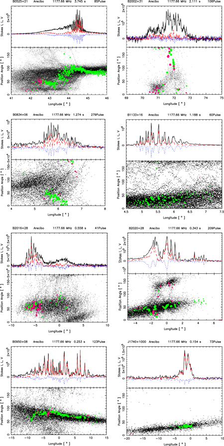
Figure 1. Collection of subpulses shown in full polarization various pulsars observed with a time resolution of 59.5 μs. In each plot the top panel shows Stokes I, L, and V in black, red, and blue lines, respectively. The polarization position angle (PPA) histogram of the entire pulse sequence is shown as a "dotty plot" display of qualifying samples in the bottom panel. The average PPA of the subpulse is plotted in green when the circular polarization is negative and magenta when positive. The ringing/modulating structures seen in the subpulses are microstructures. Note that a certain periodicity (or quasi-periodicity) is apparent in the microstructures, and all the Stokes parameters fluctuate in the same manner with the same width and periodicity.
Download figure:
Standard image High-resolution image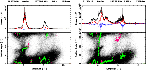
Figure 2. Two single pulses of PSR B1133+16 (plot description same as given in the caption of Figure 1), illustrating that microstructures occur within both polarization modes. In the left-hand display around 0° longitude the pulse component showing the microstructure feature corresponds to the weaker secondary polarization mode, whereas in the right-hand one at about 6° the microstructure corresponds to the primary polarization mode.
Download figure:
Standard image High-resolution image3. ESTIMATING THE MICROSTRUCTURE TIMESCALE FOR AN INDIVIDUAL PULSE
The focus of our analysis is on extracting microstructure timescales from time-series data for individual pulses. Timescales are traditionally identified as minima, maxima, or slope changes in the autocorrelation function (ACF) for a pulse. We define the (normalized) ACF at lag τ for a signal I(t) as

so that ACF(0) = 1. The behavior of the ACF needs a closer look to understand what can and cannot be inferred about the timescales of a signal. For illustration, consider the toy train of Gaussian spikes (Figure 3), which is characterized by two timescales, namely, the baseline width  of each spike, and the distance between two successive spikes, i.e., the period
  of the spike train. The gap
  between two successive spikes is assumed to be non-negative. When
  , it can be argued that the first ACF minimum occurs at lag =
  , and the first ACF maximum occurs at lag =
  . On the other hand, when
  , successive minima and maxima in the ACF are separated by the period
  of the spike train. In this regime, the ACF carries no information about the width of a spike, and we expect that the lag at the first maximum (i.e.,
  ) = 2 × the lag at the first minimum (i.e.,
  ). Conversely, any indication of the relationship
  in the inferred timescales may therefore be interpreted as suggesting the lack of complete information about the two timescales.
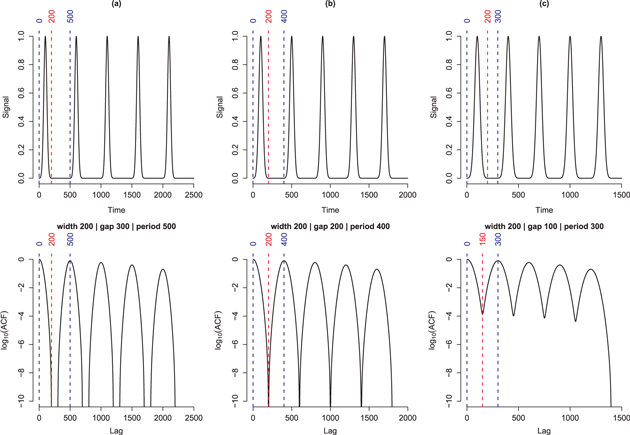
Figure 3. Toy example illustrating the relationship between the width of a spike, period of a spike train, and the first minimum and maximum in the ACF. In the top row, each spike is a truncated Gaussian with baseline width = 200, and the spike train is a sequence of equidistant spikes separated with the same gap. The period of the spike train therefore equals the widths of a spike+gap between successive spikes. (a) Width  gap; (b) width = gap; (c) width
  gap. In all cases, the first ACF maximum is at lag = period. For (a) and (b), the first ACF minimum is at lag = width, and the ACF can be used to infer both the width and period of the spike train. For (c), the first ACF minimum is at lag = period/2, and the ACF carries no information about the width. The spike train is a caricature of the microstructure feature of a subpulse and illustrates what can be inferred about timescales using the ACF. Note that the bottom row plots log10(ACF) instead of the ACF so as to accentuate the ACF minima.
Download figure:
Standard image High-resolution imageTo motivate the methodology we are about to develop for inferring microstructure timescales from individual subpulses in a pulsar data set, consider four illustrative subpulses from PSR B0525+21 together with their ACFs (Figure 4). In the left column of this figure, black curves represent probable candidates for the signal in the data time series (gray scatter), red curves represent probable candidates for the smooth trend (i.e., envelope) in the pulse, and blue curves represent probable candidates for the microstructure (obtained after removing the probable envelope from the probable signal). In the right column of this figure, the gray curves represent the ACF for the whole-pulse time series, whereas the blue curves represent the ACF for the microstructure feature. Note that while the ACF for the whole-pulse time series must be non-negative at all lags (because pulse time series are by and large positive, barring noise), the ACF for the microstructure feature may be negative (because the microstructure signal fluctuates on both sides of 0). In Figure 4, the time series for pulse 179 shows strong microstructure oscillations superimposed on top of a smooth envelope, which translate into weak but clear oscillations in the descending part of the subpulse ACF close to lag 0. For this pulse, we see that the first minimum in the subpulse ACF (gray curve in the ACF plot) agrees with the first minimum in the ACF for the microstructure feature (blue curve in the ACF plot). This pulse is an example where the conventional method of identifying microstructure timescales using the first minimum in the ACF will work flawlessly because the first minimum in the subpulse ACF is numerically well defined. The time series for pulse 37 again shows a highly fluctuating signal characteristic of the microstructure. However, the first ACF minimum is barely visible in the subpulse ACF. In contrast, the first minimum is clearly identifiable in the microstructure ACF for this pulse. The time series for pulse 21 again shows a clearly identifiable microstructure feature. However, it nevertheless leads to a featureless subpulse ACF, which makes it impossible for the conventional method to identify a microstructure timescale from it. The ACF for the microstructure feature, in contrast, has a clearly identifiable first minimum. Pulse 62 is an example where, with the exception of one or two clear but weak fluctuations in the time series, there may not be any significant/detectable microstructure feature.
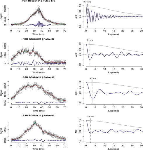
Figure 4. Few illustrative subpulses from a B0525+21 data set and their respective ACFs. Left column: gray, subpulse time series data; black, probable signal in the data sans the noise; red, probable smooth trend in the time series; blue, probable microstructure feature of the signal. Right column: gray, ACF computed directly from noisy data; blue: ACF computed from the probable microstructure feature. See text for detailed description.
Download figure:
Standard image High-resolution imageThese illustrative pulses suggest that the signal hidden in the data can be modeled as consisting of an envelope feature characterized by relatively strong long-time smooth variations and a microstructure feature characterized by relatively weak short-time quasiperiodic variations that ride on top of the envelope. Hence, with reference to the use of ACFs for identifying timescales, we expect the following two confounding situations:
- 1.The ACF of the complete pulse may be dominated by power at low frequencies, i.e., by the envelope feature, possibly masking any short-time modulations (e.g., pulses 37 and 36 in Figure 4).
- 2.Noise in the data may result in additional random oscillations in the ACF, making it numerically difficult to identify genuine minima, slope changes, etc., in the ACF for the whole subpulse.
This suggests that if the noise and the envelope feature are extracted from the data to arrive at the microstructure feature, then the microstructure feature can be used meaningfully to estimate microstructure timescales from its ACF in the conventional manner.
Therefore, a solution to the problem of estimating microstructure timescales lies in correctly estimating and removing the noise as well as the long-time smooth modulation (i.e., envelope) from a subpulse time series. Our methodology for estimating microstructure timescales from individual subpulses thus consists of the following steps:
- 1.The average pulse profiles for many pulsars are often seen to be composed of multiple emitting components. As was pointed out in some earlier studies (e.g., Soglasnov et al. 1981, 1983; Popov et al. 2002), the individual components can have different microstructure timescales. Hence, we isolate individual pulse components wherever possible before estimating timescales. Individual components are identified from the average pulse profile in the form of time windows (shown as gray sections in the figures in Appendix
B ) relative to the beginning of the profile. These windows are then applied to each single pulse in the data set to separate it into its components. For pulsars where multiple components could not be identified, we used whole pulses. Further, we restrict our analysis only to pulses with high S/N, where S/N is estimated as the ratio of the peak signal to the off-pulse noise. In Table 1, 24 pulsars marked in boldface are the ones with sufficient single-pulse S/N and hence were suitable for timescale analysis, while the others are not used. The pulsar rotational parameters for these 24 pulsars are given in Table 2. - 2.Radio-frequency interference (RFI) induced outlier values in subpulse time series data may influence timescale estimates. We therefore identify potential outliers in subpulse time-series data using a heuristic method and replace them with appropriate values resembling their respective local neighborhoods in the time series (Section
A.2 ). The decision to "curate" outliers in this fashion is made on a case-to-case basis through preliminary visual inspection of each pulsar data set. - 3.We de-noise every subpulse using a model-independent smoothing spline fit (Section
A.3 ) that adapts to the shape of the subpulse optimally. The fit thus obtained is taken to be a smooth noise-free version of the subpulse data (e.g., the black curves in Figure 4, left column). - 4.We estimate the envelope for each subpulse via kernel regression (Appendix
A.4 ) using a heuristic smoothing timescale. The difference between the fit and this envelope is the estimated microstructure. Note that the smoothing timescale (referred to as smoothing bandwidth h later on) is the most critical parameter for our methodology. Further details can be found in Section 4. - 5.The nature and strength of the microstructure feature can vary considerably among subpulses. Specifically, the microstructure feature may be nearly absent or at best weak in some of the subpulses. We identify subpulses with weak microstructure using the degrees of freedom (dof) for the smoothing spline fit (Appendix
A.3 ), because lower dof values correspond to smoother fits and weaker microstructures. For better estimation of microstructure timescales, we reject subpulses with dof in the lower 10–20 percentiles of the dof distribution for that data set (see Supplementary Table 4 for the percentile cutoff for each data set). - 6.For the selected pulses, the two characteristic microstructure timescales (width
 and period ) are estimated, respectively, as the first minimum and the first maximum in the ACF of the estimated microstructure for a subpulse. Because of the substantial variation in microstructure characteristics across subpulses, the timescales thus obtained need to be further summarized or analyzed statistically. Specifically, for each pulsar, we report the median timescale together with the median absolute deviation (MAD) as a measure of spread. We also explore the nature of any relationship between and .


Table 2. Pulsar Parameters Used for Microstructure Study in This Paper Obtained from the ATNF Catalog Available at http://atnf.csiro.au/research/pulsar/psrcat/ (Manchester et al. 2005)
| PSR | Per |

|
AGE | BSURF |

|
|
|---|---|---|---|---|---|---|
| Name | s | ( ) ) |
( Yr) Yr) |
( G) G) |
( ergs s-1) ergs s-1) |
|
| 1 | B0301+19 | 1.387584 | 1.30 | 17.0 | 1.36 | 1.91 |
| 2 | B0525+21 | 3.745539 | 40.1 | 1.48 | 12.4 | 3.01 |
| 3 | J0546+2441 | 2.843850 | 7.65 | 5.89 | 4.72 | 1.31 |
| 4 | B0656+14 | 0.384891 | 55.0 | 0.111 | 4.66 | 3810 |
| 5 | B0751+32 | 1.442349 | 1.08 | 21.2 | 1.26 | 1.42 |
| 6 | B0823+26 | 0.530661 | 1.71 | 4.92 | 0.964 | 45.2 |
| 7 | B0834+06 | 1.273768 | 6.80 | 2.97 | 2.98 | 13.0 |
| 8 | B0919+06 | 0.430627 | 13.7 | 0.497 | 2.46 | 679 |
| 9 | B0950+08 | 0.253065 | 0.23 | 17.5 | 0.244 | 56.0 |
| 10 | B1133+16 | 1.187913 | 3.73 | 5.04 | 2.13 | 8.79 |
| 11 | B1237+25 | 1.382449 | 0.96 | 22.8 | 1.17 | 1.43 |
| 12 | J1740+1000 | 0.154087 | 21.5 | 0.114 | 1.84 | 23200 |
| 13 | B1737+13 | 0.803050 | 1.45 | 8.77 | 1.09 | 11.1 |
| 14 | J1910+0714 | 2.712423 | 6.12 | 7.02 | 4.12 | 1.21 |
| 15 | B1910+20 | 2.232969 | 10.2 | 3.48 | 4.82 | 3.61 |
| 16 | B1919+21 | 1.337302 | 1.35 | 15.7 | 1.36 | 2.23 |
| 17 | B1929+10 | 0.226518 | 1.16 | 3.10 | 0.518 | 393 |
| 18 | B1944+17 | 0.440618 | 0.0241 | 290 | 0.104 | 1.11 |
| 19 | B2002+31 | 2.111265 | 74.6 | 0.449 | 12.7 | 31.3 |
| 20 | B2016+28 | 0.557953 | 0.148 | 59.7 | 0.291 | 3.37 |
| 21 | B2020+28 | 0.343402 | 1.89 | 2.87 | 0.816 | 185 |
| 22 | B2034+19 | 2.074377 | 2.04 | 16.1 | 2.08 | 0.902 |
| 23 | B2110+27 | 1.202852 | 2.62 | 7.27 | 1.80 | 5.95 |
| 24 | B2315+21 | 1.444653 | 1.05 | 21.9 | 1.24 | 1.37 |
Download table as: ASCIITypeset image
The microstructure timescale analysis pipeline developed in this paper is implemented in the R (R Core Team 2014) open source statistical computing environment. Detailed pulsarwise results are available as a tarball in ftp://ftpnkn.ncra.tifr.res.in/dmitra/hires_analysis_pdf.tar.gz or http://cms.unipune.ac.in/reports/tr-20150223/.
4. RESULTS
Figures 5 and 6 depict typical results from our analysis package. Figure 5 shows how the technique is applied to a subpulse (see caption for description). We estimate the microstructure periodicity  as the first peak in the ACF of the microstructure signal (blue line) and show the results for three envelope smoothing bandwidths h because the estimated timescales are sensitive to the envelope bandwidth, where h is the smoothing window size in units of the total number of points in a subpulse (see Section
  estimated from first peak in the ACF is easily discernible. This gave us a range of h values over which the
  value remained unchanged. Using a few representative h values in this range, we found the distributions of
  . The median value of these
  distributions (or
  found from first dip in the ACF) appeared to be in good agreement with available estimates in the literature. We found that for all pulsars, h larger than 0.1 produced envelopes that were too smooth, whereas h less than 0.05 led to envelopes that traced the subpulse data too closely. All our results are hence quoted for three representative bandwidths, namely, 0.1, 0.075, and 0.05, as illustrated in Figure 6. The median of the
  histogram is given in columns 5–7 of Table 3, where the spread of the
  distribution is estimated using the MAD. Column 2 gives the longitude range used to define the subpulses for microstructure analysis, and these can be identified from the average pulse profiles presented in Appendix
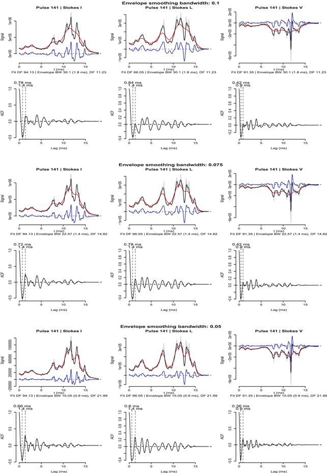
Figure 5. Analysis method for extracting the timescale of a single subpulse for the trailing component of PSR B1133+16. The plot has three columns, with each column corresponding to Stokes I, L, and V, respectively. In each column the upper panel shows the subpulse, where the gray line corresponds to the subpulse data, the black line is the fit to the data, the red line is the envelope for a given bandwidth, and the blue line is the microstructure signal defined as the difference between the red and black lines. The second panel corresponds to the ACF of the microstructure (blue) signal. The timescales that we measure are indicated in the figure. The three sets of plots from top to bottom are for three different bandwidth values 0.1, 0.075, and 0.05, respectively (see the text for details).
Download figure:
Standard image High-resolution image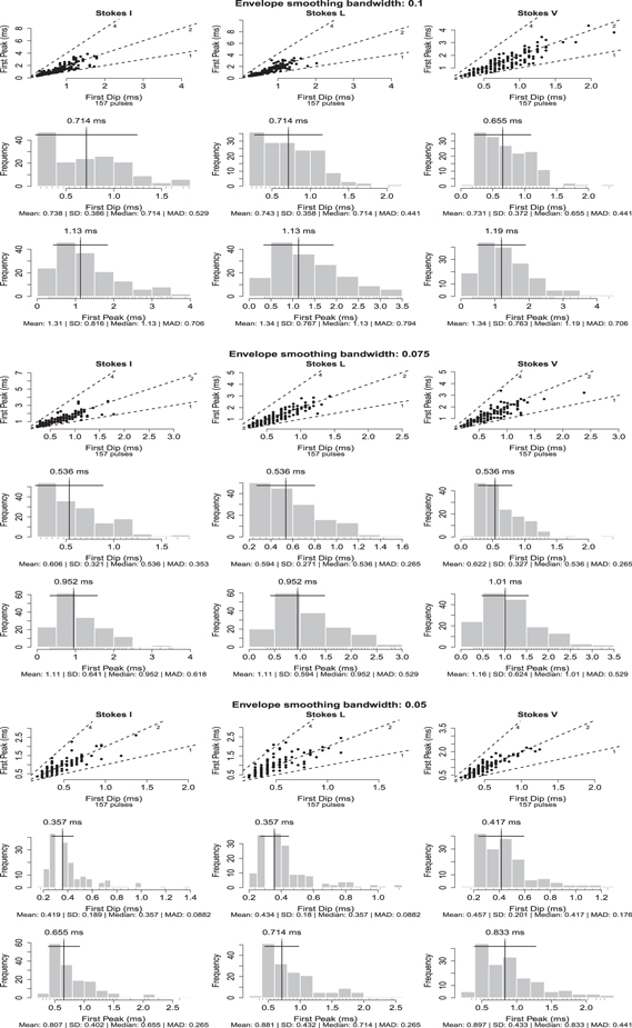
Figure 6. Histograms of the estimated timescales of the microstructure signal for the trailing component of PSR B1133+16. The three sets of plots correspond to three different bandwidths h = 0.1, 0.075, and 0.05, respectively, from top to bottom. In each plot there are three columns corresponding to Stokes I, L, and V from left to right, respectively. The topmost panel in each plot is the relation between the first dip (as x-axis) and first peak (as y-axis) of the ACF. The middle panel shows the distribution of the first dip in the ACF, which corresponds to  . The bottom panel shows the distribution of the first peak in the ACF, which corresponds to
  (see the text for details).
Download figure:
Standard image High-resolution imageTable 3.
The Median  Values for Microstructures for All the Stokes Parameters
Median  from ACF Histogram from ACF Histogram |
||||||||
|---|---|---|---|---|---|---|---|---|
| PSR | Longitude | Frequation | Period |
 |
 |

|
NPT | |
| Name | Range (°) | (GHz) | (s) | (ms) | (ms) | (ms) | h | |
| B0301+19 | −2.2–2.5 | 1.2 | 1.387 | 1.46 (0.57) | 1.49 (0.57) | 1.25 (0.35) | 0.10 | 301 |
| B0301+19 | ⋯ | 1.2 | 1.387 | 1.19 (0.44) | 1.25 (0.48) | 1.13 (0.35) | 0.075 | 301 |
| B0301+19 | ⋯ | 1.2 | 1.387 | 1.07 (0.27) | 1.01 (0.35) | 1.07 (0.35) | 0.05 | 301 |
| B0301+19 | −11.8–−5.2 | 1.2 | 1.387 | 1.73 (0.97) | 1.85 (0.88) | 2.44 (1.10) | 0.10 | 427 |
| B0301+19 | ⋯ | 1.2 | 1.387 | 1.49 (0.62) | 1.64 (0.71) | 1.96 (0.79) | 0.075 | 427 |
| B0301+19 | ⋯ | 1.2 | 1.387 | 1.22 (0.40) | 1.31 (0.40) | 1.67 (0.66) | 0.05 | 427 |
| B0525+21 | −2.85–2.86 | 1.2 | 3.745 | 4.17 (2.03) | 4.94 (2.47) | 6.01 (2.74) | 0.10 | 1001 |
| B0525+21 | ⋯ | 1.2 | 3.745 | 3.57 (1.76) | 4.23 (1.85) | 4.70 (2.21) | 0.075 | 1001 |
| B0525+21 | ⋯ | 1.2 | 3.745 | 2.98 (1.24) | 3.21 (1.50) | 3.51 (1.68) | 0.050 | 1001 |
| B0525+21 | −14.3–−10.9 | 1.2 | 3.745 | 5.65 (3.88) | 6.49 (3.44) | 7.50 (3.27) | 0.10 | 1201 |
| B0525+21 | ⋯ | 1.2 | 3.745 | 4.52 (2.47) | 5.48 (2.91) | 6.19 (3.27) | 0.075 | 1201 |
| B0525+21 | ⋯ | 1.2 | 3.745 | 3.39 (1.68) | 3.99 (2.21) | 4.46 (2.74) | 0.050 | 1201 |
| J0546+2441 | −2.13–1.81 | 1.2 | 2.843 | 2.74 (1.2) | 3.04 (1.60) | 4.23 (1.85) | 0.10 | 504 |
| J0546+2441 | ⋯ | 1.2 | 2.843 | 2.38 (0.71) | 2.44 (1.24) | 3.63 (1.85) | 0.075 | 504 |
| J0546+2441 | ⋯ | 1.2 | 2.843 | 2.14 (0.88) | 1.99 (0.84) | 2.68 (1.15) | 0.050 | 504 |
| B0656+14 | −0.61–4.95 | 1.2 | 0.384 | 0.42 (0.18) | 0.48 (0.18) | 0.72 (0.27) | 0.10 | 101 |
| B0656+14 | ⋯ | 1.2 | 0.384 | 0.42 (0.09) | 0.42 (0.09) | 0.66 (0.27) | 0.075 | 101 |
| B0656+14 | ⋯ | 1.2 | 0.384 | 0.36 (0.09) | 0.36 (0.09) | 0.60 (0.27) | 0.05 | 101 |
| B0751+32 | −2.24–2.43 | 1.2 | 1.442 | 2.58 (1.33) | 3.12 (1.33) | 3.66 (1.60) | 0.10 | 304 |
| B0751+32 | ⋯ | 1.2 | 1.442 | 2.10 (0.98) | 2.64 (1.33) | 3.42 (1.65) | 0.075 | 304 |
| B0751+32 | ⋯ | 1.2 | 1.442 | 1.86 (0.89) | 1.86 (1.20) | 2.25 (1.33) | 0.050 | 304 |
| B0823+26 | −1.65–1.41 | 1.2 | 0.530 | 0.84 (0.53) | 0.78 (0.53) | 0.90 (0.45) | 0.10 | 264 |
| B0823+26 | ⋯ | 1.2 | 0.530 | 0.72 (0.45) | 0.72 (0.36) | 0.84 (0.45) | 0.075 | 264 |
| B0823+26 | ⋯ | 1.2 | 0.530 | 0.60 (0.27) | 0.60 (0.27) | 0.72 (0.27) | 0.050 | 264 |
| B0834+06 | −1.32–1.46 | 1.2 | 1.275 | 0.78 (0.35) | 0.90 (0.46) | 1.14 (0.53) | 0.10 | 167 |
| B0834+06 | ⋯ | 1.2 | 1.275 | 0.72 (0.18) | 0.84 (0.36) | 1.02 (0.45) | 0.075 | 167 |
| B0834+06 | ⋯ | 1.2 | 1.275 | 0.60 (0.18) | 0.66 (0.27) | 0.87 (0.49) | 0.050 | 167 |
| B0834+06 | 3.7—7.2 | 1.2 | 1.275 | 1.14 (0.62) | 1.26 (0.71) | 2.22 (1.51) | 0.10 | 210 |
| B0834+06 | ⋯ | 1.2 | 1.275 | 0.96 (0.45) | 1.02 (0.53) | 1.44 (0.80) | 0.075 | 210 |
| B0834+06 | ⋯ | 1.2 | 1.275 | 0.90 (0.45) | 0.84 (0.36) | 1.17 (0.80) | 0.050 | 210 |
| B0919+06 | −7.5–4.74 | 1.2 | 0.430 | 0.96 (0.27) | 0.90 (0.27) | 1.83 (0.93) | 0.10 | 249 |
| B0919+06 | ⋯ | 1.2 | 0.430 | 0.90 (0.27) | 0.84 (0.27) | 1.44 (0.71) | 0.075 | 249 |
| B0919+06 | ⋯ | 1.2 | 0.430 | 0.78 (0.22) | 0.78 (0.27) | 1.02 (0.45) | 0.050 | 249 |
| B0950+08 | −12.77–10.84 | 1.2 | 0.253 | 0.66 (0.31) | 0.66 (0.31) | 0.72 (0.27) | 0.10 | 279 |
| B0950+08 | ⋯ | 1.2 | 0.253 | 0.63 (0.22) | 0.66 (0.27) | 0.75 (0.31) | 0.075 | 279 |
| B0950+08 | ⋯ | 1.2 | 0.253 | 0.54 (0.18) | 0.60 (0.18) | 0.66 (0.27) | 0.050 | 279 |
| B1133+16 | −1.47–3.39 | 1.2 | 1.187 | 1.01 (0.62) | 0.95 (0.44) | 1.13 (0.53) | 0.10 | 271 |
| B1133+16 | ⋯ | 1.2 | 1.187 | 0.83 (0.44) | 0.83 (0.35) | 1.01 (0.44) | 0.075 | 271 |
| B1133+16 | ⋯ | 1.2 | 1.187 | 0.71 (0.27) | 0.71 (0.27) | 0.83 (0.35) | 0.050 | 271 |
| B1133+16 | 3.39–8.8 | 1.2 | 1.187 | 1.13 (0.71) | 1.13 (0.80) | 1.19 (0.71) | 0.10 | 301 |
| B1133+16 | ⋯ | 1.2 | 1.187 | 0.95 (0.62) | 0.95 (0.53) | 1.01 (0.53) | 0.075 | 301 |
| B1133+16 | ⋯ | 1.2 | 1.187 | 0.66 (0.27) | 0.71 (0.27) | 0.83 (0.44) | 0.050 | 301 |
| B1237+25 | −2.07–4.3 | 1.2 | 1.382 | 3.06 (1.60) | 3.30 (1.42) | 3.12 (1.07) | 0.01 | 401 |
| B1237+25 | ⋯ | 1.2 | 1.382 | 2.16 (1.16) | 2.34 (1.16) | 2.58 (1.07) | 0.075 | 401 |
| B1237+25 | ⋯ | 1.2 | 1.382 | 1.38 (0.53) | 1.44 (0.71) | 2.10 (1.07) | 0.050 | 401 |
| B1237+25 | 8.77–11.87 | 1.2 | 1.382 | 1.38 (0.45) | 1.50 (0.71) | 1.98 (0.98) | 0.01 | 201 |
| B1237+25 | ⋯ | 1.2 | 1.382 | 1.26 (0.45) | 1.26 (0.45) | 1.98 (0.98) | 0.075 | 201 |
| B1237+25 | ⋯ | 1.2 | 1.382 | 1.20 (0.53) | 1.20 (0.53) | 1.53 (0.76) | 0.050 | 201 |
| J1740+1000 | −4.87–10.7 | 1.2 | 0.154 | 0.54 (0.18) | 0.54 (0.18) | 0.93 (0.44) | 0.10 | 113 |
| J1740+1000 | ⋯ | 1.2 | 0.154 | 0.48 (0.18) | 0.48 (0.18) | 0.78 (0.36) | 0.075 | 113 |
| J1740+1000 | ⋯ | 1.2 | 0.154 | 0.42 (0.09) | 0.48 (0.09) | 0.60 (0.18) | 0.050 | 113 |
| B1737+13 | −7.94–5.41 | 1.2 | 0.803 | 1.83 (1.07) | 1.95 (0.76) | 2.52 (1.20) | 0.10 | 501 |
| B1737+13 | ⋯ | 1.2 | 0.803 | 1.80 (0.80) | 1.71 (0.76) | 2.13 (0.89) | 0.075 | 501 |
| B1737+13 | ⋯ | 1.2 | 0.803 | 1.44 (0.58) | 1.47 (0.58) | 1.92 (0.71) | 0.050 | 501 |
| J1910+0714 | −1.41–3.91 | 1.2 | 2.712 | 5.71 (1.85) | 5.65 (3.18) | 6.37 (2.82) | 0.10 | 675 |
| J1910+0714 | ⋯ | 1.2 | 2.712 | 5.36 (2.21) | 4.64 (2.38) | 5.65 (3.27) | 0.075 | 675 |
| J1910+0714 | ⋯ | 1.2 | 2.712 | 4.40 (2.56) | 4.23 (2.29) | 3.81 (1.59) | 0.050 | 675 |
| B1910+20 | −1.21–6.46 | 1.2 | 2.233 | 5.74 (3.35) | 5.06 (2.12) | 5.65 (2.03) | 0.10 | 801 |
| B1910+20 | ⋯ | 1.2 | 2.233 | 4.40 (2.12) | 4.40 (1.85) | 4.82 (1.76) | 0.075 | 801 |
| B1910+20 | ⋯ | 1.2 | 2.233 | 3.78 (1.99) | 3.78 (1.81) | 4.37 (2.03) | 0.050 | 801 |
| B1919+21 | −2.45–3.10 | 1.5 | 1.337 | 1.43 (0.71) | 2.83 (1.37) | 2.92 (1.50) | 0.10 | 348 |
| B1919+21 | ⋯ | 1.5 | 1.337 | 1.31 (0.62) | 2.32 (1.15) | 2.47 (0.97) | 0.075 | 348 |
| B1919+21 | ⋯ | 1.5 | 1.337 | 1.13 (0.35) | 1.61 (0.71) | 1.93 (0.93) | 0.050 | 348 |
| B1919+21 | 5.28–8.48 | 1.5 | 1.337 | 2.20 (1.50) | 2.23 (0.84) | 2.62 (1.15) | 0.10 | 201 |
| B1919+21 | ⋯ | 1.5 | 1.337 | 1.55 (1.15) | 1.96 (0.88) | 1.96 (0.88) | 0.075 | 201 |
| B1919+21 | ⋯ | 1.5 | 1.337 | 0.77 (0.26) | 1.85 (0.26) | 1.01 (0.53) | 0.050 | 201 |
| B1929+10 | −11.1–7.84 | 1.2 | 0.226 | 0.54 (0.26) | 0.54 (0.26) | 0.54 (0.26) | 0.10 | 201 |
| B1929+10 | ⋯ | 1.2 | 0.226 | 0.48 (0.18) | 0.48 (0.18) | 0.48 (0.18) | 0.075 | 201 |
| B1929+10 | ⋯ | 1.2 | 0.226 | 0.42 (0.09) | 0.42 (0.18) | 0.48 (0.18) | 0.050 | 201 |
| B1944+17 | −9.67–4.91 | 1.2 | 0.440 | 0.77 (0.27) | 0.77 (0.35) | 1.13 (0.57) | 0.10 | 301 |
| B1944+17 | ⋯ | 1.2 | 0.440 | 0.71 (0.18) | 0.77 (0.27) | 0.95 (0.44) | 0.075 | 301 |
| B1944+17 | ⋯ | 1.2 | 0.440 | 0.71 (0.18) | 0.71 (0.18) | 0.77 (0.27) | 0.050 | 301 |
| B2002+31 | −2.48–2.01 | 1.2 | 2.111 | 1.31 (0.71) | 1.73 (0.71) | 2.20 (0.62) | 0.10 | 445 |
| B2002+31 | ⋯ | 1.2 | 2.111 | 1.25 (0.53) | 1.67 (0.62) | 2.02 (0.62) | 0.075 | 445 |
| B2002+31 | ⋯ | 1.2 | 2.111 | 1.01 (0.35) | 1.43 (0.44) | 1.85 (0.62) | 0.050 | 445 |
| B2016+28 | −5.34–4.45 | 1.2 | 0.557 | 0.66 (0.18) | 0.66 (0.18) | 0.86 (0.40) | 0.10 | 256 |
| B2016+28 | ⋯ | 1.2 | 0.557 | 0.66 (0.18) | 0.66 (0.18) | 0.83 (0.27) | 0.075 | 256 |
| B2016+28 | ⋯ | 1.2 | 0.557 | 0.66 (0.18) | 0.66 (0.18) | 0.71 (0.27) | 0.050 | 256 |
| B2020+28 | −11.27–−5.03 | 1.2 | 0.343 | 0.66 (0.27) | 0.66 (0.27) | 0.60 (0.18) | 0.10 | 101 |
| B2020+28 | ⋯ | 1.2 | 0.343 | 0.60 (0.27) | 0.60 (0.27) | 0.54 (0.18) | 0.075 | 101 |
| B2020+28 | ⋯ | 1.2 | 0.343 | 0.48 (0.18) | 0.48 (0.18) | 0.48 (0.18) | 0.050 | 101 |
| B2020+28 | −3.78–1.21 | 1.2 | 0.343 | 0.54 (0.27) | 0.60 (0.27) | 0.60 (0.27) | 0.10 | 98 |
| B2020+28 | ⋯ | 1.2 | 0.343 | 0.48 (0.18) | 0.54 (0.18) | 0.54 (0.18) | 0.075 | 98 |
| B2020+28 | ⋯ | 1.2 | 0.343 | 0.42 (0.09) | 0.42 (0.18) | 0.48 (0.18) | 0.050 | 98 |
| B2034+19 | −5.25–−1.49 | 1.2 | 2.074 | 3.36 (1.24) | 3.12 (1.10) | 3.04 (1.24) | 0.10 | 361 |
| B2034+19 | ⋯ | 1.2 | 2.074 | 3.10 (1.50) | 2.86 (1.15) | 2.92 (1.37) | 0.075 | 361 |
| B2034+19 | ⋯ | 1.2 | 2.074 | 2.80 (1.68) | 2.62 (1.06) | 2.80 (1.41) | 0.050 | 361 |
| B2110+27 | −1.3–2.26 | 1.47 | 1.202 | 1.19 (0.09) | 1.25 (0.09) | 1.19 (0.44) | 0.10 | 201 |
| B2110+27 | ⋯ | 1.47 | 1.202 | 1.13 (0.09) | 1.19 (0.09) | 1.07 (0.35) | 0.075 | 201 |
| B2110+27 | ⋯ | 1.47 | 1.202 | 1.07 (0.18) | 0.95 (0.27) | 0.83 (0.18) | 0.050 | 201 |
| B2315+21 | −1.79–1.17 | 1.47 | 1.444 | 1.07 (0.09) | 1.01 (0.09) | 1.19 (0.35) | 0.10 | 201 |
| B2315+21 | ⋯ | 1.47 | 1.444 | 1.01 (0.09) | 1.01 (0.09) | 1.07 (0.27) | 0.075 | 201 |
| B2315+21 | ⋯ | 1.47 | 1.444 | 0.95 (0.09) | 0.95 (0.18) | 0.83 (0.18) | 0.050 | 201 |
Notes. In column 2 the longitude range is the window that has been used for analysis, and this region of the pulse can be seen as gray regions in the average profiles given in the appendices. In columns 5–7 the median  value is given, and the values in parentheses, correspond to the median absolute deviation of the
  values. Column 8 gives the value of the bandwidth h used for analysis, and column 9 gives the number of points in the pulse window (see, the text for further details).
The top panel of each plot in Figure 6 deserves attention. The plot depicts the relationship between the values of the first dip ( ) along the x-axis and the first peak (
 ) along the y-axis as estimated from the ACFs of the microstructure. The three dotted lines correspond to
  , and
, and  , respectively. Most of the points in this figure (and also for other pulsars) are seen to cluster around the
  line, indicating that the microstructure is unresolved and hence the width
  cannot be determined.
Before we close this section, it is important to compare our analysis method with earlier studies. A majority of the studies use the first dip or peak of the ACF to estimate microstructure timescales (e.g., Hankins 1972; Soglasnov et al. 1981). However, as mentioned earlier, the broad subpulse power and noise in the subpulse make it difficult to extract the timescales numerically. Our method is designed to alleviate these problems by first de-noising the subpulse profile and then removing a smooth envelope from it. Other studies have used the power spectrum to estimate timescales corresponding to quasi-periodic microstructures (e.g., Lange et al. 1998; Popov et al. 2002). The slow-varying envelope in these cases appears as low-frequency power in the spectrum. For example, Popov et al. (2002) construct the ACF by cross-correlating the voltages from two different spectral channels, while Lange et al. (1998) use the derivative of the power spectrum, although noise in single pulses may still affect their analyses. The strength of our method lies in its ability to recover low-amplitude intensity modulations in a subpulse, isolating the microstructure from the subpulse time series. Consequently, we find that a majority of the subpulses have microstructure emission superposed on a smooth broad emission (envelope).
5. DISTRIBUTION OF TIMESCALES FOR ALL STOKES PARAMETERS AND THE –P RELATION

Cordes (1979), based on 10 pulsars observed at 430 MHz in the pulsar period range of 0.2–3.7 s, found the relationship  between the microstructure timescale
  and the pulsar period P. Kramer et al. (2002) reestablished this relationship as
  using 12 pulsars where
  estimates were available in the literature for different frequencies. With our current set of observations we are in a position to revisit this relationship using 24 pulsars at L band. Since broad microstructures cannot be resolved, we believe that the periodicity
  is a more relevant quantity instead of
  . Figure 7 plots the median value of
  against period P. The top panel corresponds to the total intensity, the middle one to the linear polarization, and the bottom one to the circular. The
  points are estimated from the median value of the histogram of the first peak in the ACF, and the error bars reflect the MAD of the
  distribution. A linear fit of the form
  was performed using the median
  values for Stokes I corresponding to h = 0.1, 0.075, and 0.05 separately, which yielded (m, c) values as
  , and
, and  respectively. These fits are shown in Figure 7. We note that the fit is merely demonstrating the tendency that median
  increases with increasing pulsar period P, although a large spread of
  values exists for all pulsars.

Figure 7. Filled points and the error bars in the above plots are the median value and the median absolute deviation of  distribution given in Table 3 for all the pulsars as a function of pulsar period P. The three plots from top to bottom correspond to Stokes I, L, and V, respectively. The red, green, and blue points correspond to bandwidths of 0.1, 0.075, and 0.05, respectively. The dashed red, green, and blue lines are a fit to the median
  values for Stokes I corresponding to bandwidth 0.1, 0.075, and 0.05, respectively. The same lines are shown for Stoke L and V for reference. The orange line at 300 μs along the abscissa is about five times the time resolution of our observations.
Download figure:
Standard image High-resolution imageCorrelation of  with other pulsar rotational parameters like period derivative, characteristic age and surface magnetic field did not show any significant trends. Although a weak anticorrelation was seen (not shown here) between the slowdown energy (
 ) and
) and  , more data are needed to establish this.
6. HOW DOES BROAD MICROSTRUCTURE AVERAGE TO FORM A SUBPULSE?
It was evident from early polarization observations (e.g., Clark & Smith 1969; Manchester et al. 1975) that single pulses are highly linearly polarized and that the circular polarization changes sign or handedness within a pulse. Based on high-quality single-pulse polarimetry, Mitra et al. (2009, hereafter MGM09) have showcased a collection of subpulses from an assorted set of pulsars, where the subpulses had a Gaussian shape, with close to 100% linear polarization and associated with sign-changing circular. One such example is shown in the left panel of Figure 8.

Figure 8. Left: subpulse of PSR B2020+28 (plot description same as given in the caption of Figure 1), which has been smoothed to a time resolution of 595 μs. Note that the subpulse is close to 100% linearly polarized and shows a sign-changing circular. Right: high-resolution pulse with time resolution 59.5 μs. The striking point to note there is that the subpulse is split into microstructures, with the linear and circular polarization following the same width and periodicity as that of the total intensity. These microstructures hence do not represent coherent curvature radiation by charged bunches in vacuum (see the text for details).
Download figure:
Standard image High-resolution imageFor a long time this emission pattern kindled great interest in the pulsar community (see, e.g., Michel 1987; Radhakrishnan & Rankin 1990), because this remarkably resembles the emission pattern due to single-particle vacuum curvature radiation as the observer cuts across the emission cone (i.e., the 1/γ cone). The mathematical formulation for obtaining Stokes parameters due to curvature radiation in vacuum for a single relativistically moving particle has been explicitly calculated by several authors (e.g., Gil & Snakowski 1990a, 1990b; Ahmadi & Gangadhara 2002). Let us recall the polarization properties of single-particle curvature radiation in vacuum based on the description given by Gil & Snakowski (1990a, 1990b). Consider a charged particle moving relativistically with Lorentz factor γ, along super-strong magnetic field lines, with a radius of curvature ρ. The particle will emit curvature radiation beamed in the forward direction. The Fourier components of the electric fields can be decomposed into parallel ( ) and perpendicular (
 ) components to the plane of the curved magnetic field lines (see Equations (7) and (8) of Gil & Snakowski 1990a). When the radiation is viewed as a cut through the emission beam, the
  has a sinusoidal form, and
  is positive and has a relative phase shift of 90°, forming an orthogonal basis. The radiation polarized in the parallel and perpendicular direction is also known as the ordinary (O) and extraordinary (X) modes. The power in curvature radiation is dependent on the frequency of emission and achieves its maximum at
  , the characteristic frequency that is given by
  in the vacuum case (see Figure 2 of Gil & Snakowski 1990b). The ratio of the two components, as well as the width of the pulse, is dependent on both the viewing angle φ and the frequency of emission (see Figures 3–5 of Gil & Snakowski 1990b). The width of the pulse is approximately equal to
  at
at  . The power in the O mode is seven times stronger than the X mode in vacuum (Jackson 1975; Gil et al. 2004).
Our aim here is to look for signatures of the aforementioned vacuum curvature radiation in the data. First, let us note that the subpulse width cannot be associated with the elementary 1/γ emission cone, because when observed with higher time resolution, the subpulse splits into microstructures. In an attempt to reproduce this subpulse radiation pattern, Gil & Snakowski (1990a) and Gil et al. (1993) used the shot-noise model of pulsar emission, where the subpulse is an incoherent addition of smaller bunches, with each bunch emitting like a single-particle vacuum curvature radiation. The subpulse shape results from the intensity gradient due to the charge density variation of the bunches across the subpulse. These authors demonstrated that in the presence of intensity gradients, the resulting emission will have a net circular polarization as observed in subpulses. The beams from the bunches do not overlap, so the linear polarization remains high. Assuming  , and therefore an angular size
  for the emitting bunches, they simulated several pulses that appear similar to the subpulses showcased by MGM09. These results were also recently confirmed by Gangadhara (2010). A prediction of this model is that if a subpulse can be resolved into microstructures (e.g., see Figure 3 of Gil et al. 1993), then the microstructure should have features that mimic the single-particle vacuum curvature-radiation pattern. To test this theory, we need examples of subpulses where the microstructures are highly resolved. Note that the subpulses chosen should be highly linearly polarized such that they do not suffer from any depolarization effects due to orthogonal polarization moding5
or due to an incoherent addition from an overlapping
for the emitting bunches, they simulated several pulses that appear similar to the subpulses showcased by MGM09. These results were also recently confirmed by Gangadhara (2010). A prediction of this model is that if a subpulse can be resolved into microstructures (e.g., see Figure 3 of Gil et al. 1993), then the microstructure should have features that mimic the single-particle vacuum curvature-radiation pattern. To test this theory, we need examples of subpulses where the microstructures are highly resolved. Note that the subpulses chosen should be highly linearly polarized such that they do not suffer from any depolarization effects due to orthogonal polarization moding5
or due to an incoherent addition from an overlapping  emission beam (see MGM09).
In the left panel of Figure 8, a subpulse of PSR B2020+28 is shown that is highly linearly polarized and is associated with a sign-changing circular polarization, similar to the pulses showcased by MGM09. The right panel shows the high-time-resolution data for the same subpulse, and clearly resolved microstructures are seen. As expected, the linear polarization of the individual microstructures is close to 100% in order to produce the highly polarized subpulse. The circular polarization below the microstructure feature does not show any sign reversals. Rather, it has the same width (and also periodicity) as the total intensity and linear polarization. In fact, this description is true for all subpulses where sufficiently resolved microstructures are seen. Figure 1 shows several such examples, and very clear examples where Stokes V has the same  as Stokes I and L are shown in Figure 9. This feature is also borne out from the statistical analysis of the data set where the median
  values of Stokes I, L, and V are similar, as can be seen in Table 3. Thus, based on these observations, one is compelled to conclude that the radiation pattern of resolved microstructures is not consistent with single-particle curvature radiation of charged bunches in vacuum. In the next section, we will discuss how these findings corroborate our current understanding of the pulsar emission mechanism.
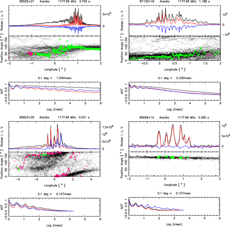
Figure 9. Few archetypal examples (as in Figure 1) illustrating that the circular polarization follows the same  values as the total intensity and linear polarization. In each display a highly resolved subpulse is shown, and in the bottom panel the ACFs of the Stokes parameters are shown. Note that in all the examples the PPA across the subpulse is primarily associated with a single polarization mode. Clearly the ACFs of Stokes I, L, and V trace each other extremely well.
Download figure:
Standard image High-resolution image7. PULSAR MICROSTRUCTURE AND ITS IMPLICATIONS FOR THE COHERENT RADIO EMISSION MECHANISM
Coherent pulsar radio emission can be generated by means of either a maser or coherent curvature mechanism (Ginzburg & Zhelezniakov 1975; Kazbegi et al. 1991; Melikidze et al. 2000, hereafter MGP00). There is general agreement that this radiation is emitted in curved magnetic field-line planes due to growth of plasma instabilities in the strongly magnetized electron–positron plasma well inside the light cylinder. Many observational constraints on the emission altitude suggest that the emitted radiation detaches from the ambient plasma at altitudes of about 500 km above the stellar surface, which is typically less than 10% of the light-cylinder radius  (e.g., Cordes 1978; Blaskiewicz et al. 1991; Rankin 1993; Kijak & Gil 1997; Mitra & Deshpande 1999; Gangadhara & Gupta 2001; Mitra & Li 2004; Krzeszowski et al. 2009). The magnetic field at these altitudes is so strong that the plasma is constrained to move only along the magnetic field lines. Under such conditions, the two-stream instability is the only known instability that can develop, and the growth of this plasma instability leads to the formation of charged relativistic solitons, which can excite coherent curvature radiation in the plasma (e.g., Asseo & Melikidze 1998; Melikidze et al. 2000; Gil et al. 2004, hereafter GLM04).
The basic requirement of the theory of coherent radio emission is the presence of a non-stationary inner acceleration region. Ruderman & Sutherland (1975, hereafter RS75) were among the first to explore the conditions in the pulsar magnetosphere that lead to the formation of an inner accelerating region (also known as an inner vacuum gap, IVG) just above the pulsar polar cap where the free flow of charge is hindered, thus resulting in the formation of an IVG with a large potential difference. The physics of IVG formation can be found in RS75, and here we point out that the original RS75 IVG was not consistent with X-ray observations and radio subpulse drifting observations, and currently it is thought that a partially screened IVG exists close to the neutron star surface (Gil et al. 2003). The process that generates non-stationary flow of charges in the gap is as follows. The IVG is initially discharged by a photon-induced electron–positron pair-creation process in the strong curved magnetic field. The height (hg) of the gap stabilizes typically at about a few mean-free paths of the pair-production process. The electric field in the gap causes separation of the electrons and positrons (also known as primary particles), where the electrons bombard onto the neutron-star surface, and the positrons are accelerated away toward the outer magnetosphere. As these primary particles move, they accelerate and create further secondary particles, resulting in a pair-creation cascade. The outflowing particles are hence composed of primary particles with Lorentz factors of about 106 and secondary plasma clouds with a distribution of Lorentz factors of about 10–1000, but peaking around 300–500. This process eventually occurs over a set of magnetic field lines, and this overall spread of the discharging process is called a spark. As the electron moves toward the polar cap, it experiences  drift, causing the sparking discharge to move slowly across the polar cap. RS75 envisaged that the IVG is discharged in the form of closely packed isolated sparks, where the lateral size and distance between the sparks are equal to the gap height. A plasma column is associated with each spark, and in the radio-emission region coherent spark-associated plasma columns radiate and generate the observed subpulses in pulsars. The sparking process continues for a time ts until the whole potential in the gap is screened out, after which the plasma empties the gap in a time
  and once again the sparking process starts almost in the same place on a timescale
  (Gil & Sendyk 2000). This process results in a non-stationary flow of plasma clouds associated with every spark anchored to a specific location on the polar cap. The physics of the sparking discharge process is still a topic of active research; however, most studies suggest that in normal pulsars hg is of the order of about 50–100 m, and to screen the gap potential around 50, pair creations are needed; hence,
  μs. Note that during the time ts the
  drift causes the spark to move only very slightly across the polar cap. Two successive plasma clouds, with each cloud extending for about 50hg and separated by a distance hg, eventually overlap when the fast-moving particles of the second cloud catch up with the slow-moving particles of the first cloud, leading to the development of the two-stream instability. The instability in the plasma generates Langmuir plasma waves, and the modulational instability of the Langmuir waves leads to the formation of a large number of charged solitons that can excite extraordinary (X) and ordinary (O) modes of curvature radiation in the plasma cloud, as shown by MGP00 and GLM04. The condition for coherent emission requires the wavelength of emission to be greater than the intrinsic soliton size, i.e.,
  , where
  is the plasma frequency (see MGP00; GLM04) and
  is the Lorentz factor of the secondary plasma. The emerging radiation is an incoherent addition of the radiation emitted by each soliton.
We now discuss aspects of the soliton coherent-curvature radiation theory that relate to the two important microstructure behaviors discussed in this paper, namely, the periodic structures observed in pulsar subpulses, their linear dependence with pulsar period, and the absence of signatures of vacuum curvature radiation in pulsar microstructures. Obviously the timescales involved in the radiation process are far too small to be seen in our 59.5 μs observations; hence, we rule out that the periodic microstructures correspond to emission from individual plasma clouds or solitons.6
Another way of sampling a periodic structure would be if temporal modulation of the emission exists in the emission region. There are theoretical studies in the literature that attempt to interpret microstructure based on nonlinear plasma effects leading to temporal modulation of the pulsar emission (e.g., Chian & Kennel 1983; Asseo 1993; Weatherall 1998); however, these models are mostly developed for emission where  , whereas coherent emission requires
  .
.
The other important aspect of our observations is the absence of a signature of vacuum curvature radiation in pulsar microstructures. The coherent curvature radiation by charged bunches called "solitons" excites the extraordinary and ordinary mode in the electron–positron plasma. Due to the strong ambient magnetic field, the X-mode does not interact with the plasma and hence can escape the plasma and reach the observer (MGM09; Melikidze et al. 2014). The fate of the O-mode is, however, unclear. It has been suggested that it can be damped and gets ducted along the magnetic field lines, or if there are sharp plasma boundaries that it can escape as electromagnetic waves and reach the observer. In any case, due to propagation effects in the plasma, the X- and O-modes separate in phase and hence they do not maintain any phase relation as they emerge from the plasma. As a result, the circular polarization can no longer have any sign-changing signature as in the vacuum case. Also incoherent addition of a large number of solitons would tend to cancel any circular polarization, particularly in our observations. Thus, the origin of circular polarization still remains to be understood in this model of pulsar emission.
8. SUMMARY
In this work we have found several distinguishing features of pulsar microstructures. These can be summarized as follows:
- 1.Almost all subpulses show a quasiperiodic structure riding on top of a broad pulse envelope. In general, this structure is weak, except in occasional cases when deep modulations are seen. However, the absence of microstructure in pulsar average profiles is a clear indication that at any given longitude pulsar emission is random and stochastic.
- 2.Microstructures are also seen to be associated with both the orthogonal polarization modes.
- 3.We did not find any case where microstructure widths are resolved. In other words, we find that (where the estimated width is found as the first dip in the ACF) is related to the periodicity (found as the first peak in the ACF) (see Section 3 for details).
- 4.For every pulsar the values extracted from a collection of subpulses have a distribution, and the median value of linearly increases with pulsar period (see Section 5).
- 5.All the Stokes parameters have the same periodicity—i.e., they have the same values (see Section 6).


A variety of analysis techniques to extract microstructure timescales have been deployed in the past. The methods use either the ACF first dip and first peak or the peaks in the power spectra for estimating timescales. However, these methods are often unable to extract low-amplitude wiggles that are a quintessential feature of the subpulse microstructure, nor are they able to handle the large variability in the subpulse shapes effectively. We address these problems by de-noising the subpulse signal using a model-independent smoothing spline fit (Appendix
These quasi-periodic structures, which show a linear dependence on rotation period, cannot be understood in terms of the current theories of pulsar emission. We also find that the linear and circular polarizations follow the same distribution of timescales as the total intensity. This, as we have argued strongly, rules out the possibility that microstructures are basic units of curvature radiation in vacuum. We conclude that the microstructures within the pulsar signal reflect temporal modulations of plasma processes of the emission engine. While this paper is an exercise in understanding the properties of pulsar microstructures, theoretical progress needs to be made to understand this unique phenomenon.
We thank the anonymous referee for his/her thorough review and highly appreciate the comments and suggestions that significantly improved the paper. We thank George Melikidze and Janusz Gil for useful discussions. We also thank M. Popov for his comments on the paper. D.M. would like to thank Cornell University for extending a visiting staff position at the Arecibo Observatory, during which many of the observations reported in this paper were carried out. We would like to thank Arun Venkataraman for his many helps and services, as well as the other staff of Arecibo Observatory for support. Much of the work was made possible by support from the US National Science Foundation grants 08-07691 and 09-68296. Arecibo Observatory is operated by SRI International under a cooperative agreement with the National Science Foundation, and in alliance with Ana G. Méndez-Universidad Metropolitana and the Universities Space Research Association. This work made use of the NASA ADS astronomical data system. M.A. was supported by the National Centre for Radio Astrophysics, TIFR, as a visiting scientist during 2011-13.
APPENDIX A: METHODS
A.1. Models for Data and Noise
The measured signal Yi at time ti is modeled as

where f embodies the true but unknown variation of the subpulse signal with time and  represents the noise in the data. The N time points ti where signal is measured are assumed to be equidistant, i.e., of the form
  , where
  (δ = 59.5 μs is the time resolution for all the data sets analyzed in this work). Without loss of generality, we take
  (which amounts to redefining the time unit). The noise variables
  are assumed to be independent with mean 0 and a (constant) variance
  . Our present analysis does not require an estimate of the noise variance explicitly (except for the purpose of choosing high-S/N pulses; see Section 3). We have modeled the true signal f underlying the subpulse data as

where e and m respectively represent a smooth slow-varying envelope and faster-scale quasiperiodic modulations corresponding to microstructure. The methodology in Section A.3 is used to estimate f optimally, whereas e is estimated using the method in Section A.4. The difference  is taken to be the estimated microstructure. Figure 4 shows examples of such fit-envelope-microstructure decomposition for a few subpulses. The model A1 is inspired by the observation based on Figure 4 that the ACF is dominated by the envelope features which should be removed from the data to extract the microstructure.
A.2. Outliers
RFI over timescales that are much smaller than the pulse period may introduce isolated outliers in the subpulse time series, which may have a detrimental effect on the downstream analysis. For example, outliers may cause fluctuations in the fit that may have an effect on the ACF used for timescale identification. Therefore, before engaging into any further analysis, we first assess the extent of contamination in a data set (through visual inspection of subpulses), and, if deemed necessary, we identify (and "curate") potential outliers in all the subpulse time series in the data set heuristically as explained below. In this work, we have used this approach because of its simplicity. However, we note that a better alternative to this heuristic approach could be the use of robust nonparametric regression methods (Härdle 1992; Efromovich 1999) that deal with outliers in the regression context in a unified manner, or outlier identification methods with well-established formal properties.
Figure 10 shows examples of subpulses (#42, #44, #45) with clear outliers from a PSR B0525+21 data set. In fact, this was the only data set in the present study that showed clear outliers. Further, for this data set, it was known that these outliers were caused by radio communication from a satellite in the field of view. Figure 10 also shows a subpulse (#298) from the same data set that illustrates a failure of our heuristic method for outlier identification. This subpulse has strong and highly ringing microstructure that results in too many data points in the ringing part being wrongly tagged as potential outliers. Since we expect at most a few isolated outliers in any subpulse (say, less than 1% of the subpulse length), such over-identification can be easily detected. Outlier correction, as described below, is not applied to such subpulses.

Figure 10. Subpulses 42, 44, 45, and 298 from a PSR B0525+21 data set illustrating the behavior of our heuristic outlier identification method. See Section A.2 for description.
Download figure:
Standard image High-resolution imageIdentifying potential outliers. When the data contain an unknown trend f, it is necessary to identify a potential outlier with respect to data values in its local neighborhood. Therefore, we first obtain a pilot fit  through kernel regression (Härdle 1992; Wasserman 2006). The smoothing bandwidth for this pilot fit may be taken as a constant b times the optimal smoothing bandwidth obtained via cross-validation; slight oversmoothing (
 ) is expected to help make the fit
  somewhat robust against outliers. Any data point i with a relatively large residual
  is a potential outlier. Specifically, following the standard prescription (Frigge et al. 1989), the ith data point is tagged as a potential outlier if
  or
or  , where r75 and r25 are respectively the 75 and 25 percentile points for the residual vector (
 is therefore the interquartile range). The value of the multiplier a is taken to be 3 instead of the conventional 1.5 to make outlier identification more conservative.
Imputing potential outliers back into data. We replace a potential isolated outlier value Yi by the median of signal values in a small local neighborhood of ti. In this work, we have taken the size of the local neighborhood to be 5 points on either side of ti. That is, we replace a potential outlier value Yi with the median of  , with data boundaries handled by truncation.
A.3. Model-independent Fit to Subpulse Time-series Data
The immense variability in the pulse shapes suggests that the separation of probable signal from noise is best done using a nonparametric regression method that only makes mild assumptions about the true but unknown regression function without pre-specifying its mathematical form. In particular, we use smoothing spline regression (Green & Silverman 1994), which may be seen as a penalized least-squares method with a penalty on the roughness of the fit. An optimal value for the smoothing parameter is chosen using the standard method of (generalized) cross-validation. The smoothness of the resultant fit can be expressed in terms of dof. The dof can be interpreted as the effective number of free parameters of the fit. Specifically, a fit with greater fluctuation has larger dof, while a smoother fit has smaller dof.
A.4. Estimating the Pulse Envelope
We use the Nadaraya–Watson kernel smoother (Härdle 1992; Wasserman 2006) to estimate the envelope of a subpulse by judiciously oversmoothing the data. Through trial and error, we found that the smoothing bandwidth  is more or less reasonable for all the pulsar data sets we analyzed. However, considering that the smoothing bandwidth for the envelope is perhaps the most critical parameter of our methodology, and that there does not appear to be any principled way of arriving at a prescription for it, we report results for a number of values of
  over a plausible range; the rational for this range is discussed in Section 4.
APPENDIX B: PLOTS FOR AVERAGE PROFILES
The average profiles and polarization position angle (PPA) histograms for all the pulsars used for microstructure analysis (given in boldface in Table 1) are presented in Figures 11–16.

Figure 11. PPA histograms for pulsars B0301+19, J0546+2441, B0525+21, and B0656+14 observed with time resolution of 59.5 μs, where the instrument and band are indicated above each plot. The upper panels give the total power (black), total linear (red), and circular polarization LH-RH (blue). The lower panels give the polarization-angle density as black dots and the average PPA as red points. The gray vertical bars correspond to the longitude range for which microstructure analysis is done (see Section 4 for details).
Download figure:
Standard image High-resolution image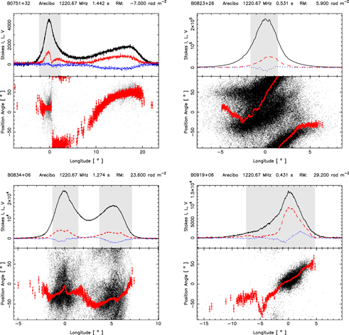
Figure 12. PPA histograms as in Figure 11 for pulsars B0751+32, B0823+26, B0834+06, and B0919+06 observed with time resolutions of 59.5 μs.
Download figure:
Standard image High-resolution image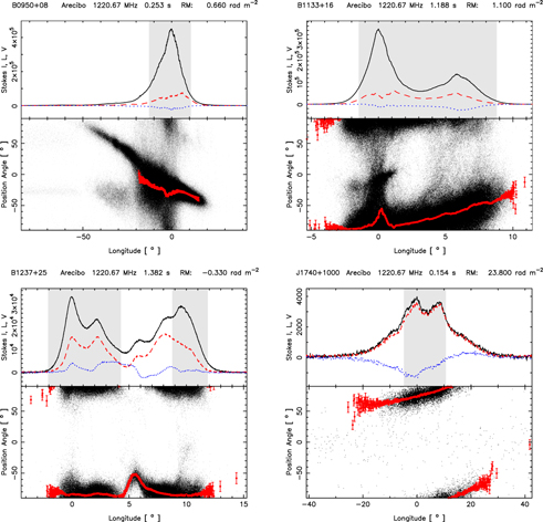
Figure 13. PPA histograms as in Figure 11 for pulsars B0950+08, B1133+16, B1237+25, and J1740+1000 observed with time resolutions of 59.5 μs.
Download figure:
Standard image High-resolution image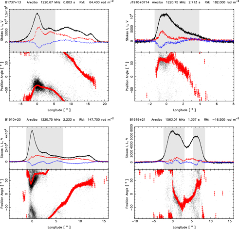
Figure 14. PPA histograms as in Figure 11 for pulsars B1737+13, J1910+0714, B1910+20, and B1919+21 observed with time resolutions of 59.5 μs.
Download figure:
Standard image High-resolution image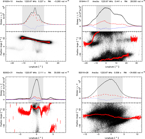
Figure 15. PPA histograms as in Figure 11 for pulsars B1929+10, B1944+17, B2002+31, and B2016+28 observed with time resolutions of 59.5 μs.
Download figure:
Standard image High-resolution image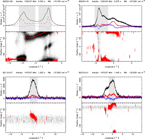
Figure 16. PPA histograms as in Figure 11 for pulsars B2020+28, B2034+19, B2110+27, and B2315+21 observed with time resolutions of 59.5 μs.
Download figure:
Standard image High-resolution image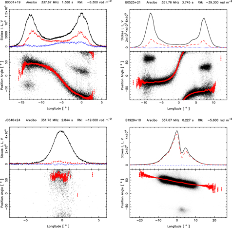
Figure 17. PPA histograms for pulsars PSR B0301+19, B0525+21, J0546+2441, and B1929+10 observed with time resolution of 59.5 μs, where the instrument and band are indicated above each plot. The respective upper panels give the total power (black), total linear (red), and circular polarization LH-RH (blue). The lower panels give the polarization-angle density as black dots and the average PPA as red points.1 of 4 images
Download figure:
Standard image High-resolution image
Figure 18. PPA histograms as in Figure 11 for pulsars B1919+21, B1944+17, B2016+28, and B2044+15 observed with time resolutions of 59.5 μs.
Download figure:
Standard image High-resolution image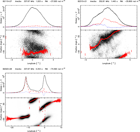
Figure 19. PPA histograms as in Figure 11 for pulsars B2110+27, B2315+21, and B2020+28 observed with time resolutions of 59.5 μs.
Download figure:
Standard image High-resolution image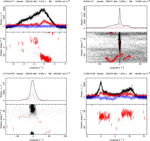
Figure 20. PPA histograms as in Figure 11 for pulsars J1503+2111, B1534+12, J1713+0747, and J1720+2150 observed with time resolutions of 59.5 μs.
Download figure:
Standard image High-resolution image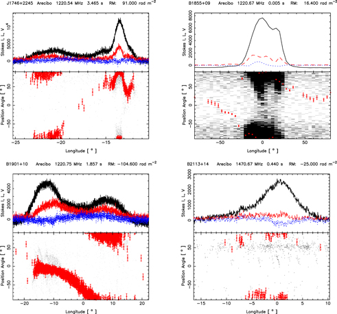
Figure 21. PPA histograms as in Figure 11 for pulsars J1746+2245, B1855+09, B1901+10, and B2113+14 observed with time resolutions of 59.5 μs.
Download figure:
Standard image High-resolution image
APPENDIX C: SUPPLEMENTAL MATERIAL: RESULTS OF PULSAR MICROSTRUCTURE ANALYSIS
The results of our pulsar microstructure timescale analysis pipeline (as described in Section 3 and Appendix of the main paper) are available for download as a tarball with the URL
ftp://ftpnkn.ncra.tifr.res.in/dmitra/hires_analysis_pdf.tar.gz
or
http://cms.unipune.ac.in/reports/tr-20150223/
Untarring this tarball creates the directory hires_analysis_pdf/. This directory contains two pdf files for each pulsar data set analyzed, with names of the form
<dataset>-<envelope_smoothing_bandwidth>-pulses3.pdf,
containing pulsewise fit, envelope, microstructure, and ACF plots (where rejected pulses are indicated using gray shading overlaid on plots), and
<dataset>-<envelope_smoothing_bandwidth>-hist3.pdf,
containing microstructure timescale histograms. For example, the files B0301+19LC-0p05-pulses3.pdf and B0301+19LC-0p05-hist3.pdf respectively contain pulsewise plots and microstructure timescale histograms for the data set B0301+19LC when analyzed using envelope smoothing bandwidth h = 0.05.
APPENDIX D: SUPPLEMENTAL MATERIAL: ASCII PROFILES
The average profiles obtained for our microstructure observations can be downloaded as ascii profiles from ftp://ftpnkn.ncra.tifr.res.in/dmitra/hires_ascprof.tar.gz
or
http://cms.unipune.ac.in/reports/tr-20150223/ as a tarball. Untarring the tarball creates a directory "asc_profiles" that has the ascii files for each pulsar. A README file describes the contents of the files.
APPENDIX E: SUPPLEMENTAL MATERIAL: PLOTS FOR AVERAGE PROFILES
The average profiles and polarization position angle (PPA) histograms for the pulsars that were not used for microstructure analysis (given as non-boldface pulsars in Table 1) are presented in Figures 17–21.
Table 4. Additional details on the data sets analyzed (compare with Table 2, main paper).
| No. | Data Set | Longitude | # of Pulses in | NPT | Outliers | Percentile |
|---|---|---|---|---|---|---|
| Range (°) | the Data Set | Curated? | Cut off | |||
| 1. | B0301+19 | −2.2—2.5 | 120 | 301 | N | 10 |
| 2. | B0301+19LC | −11.8—−5.2 | 129 | 427 | N | 10 |
| 3. | J0546+2441 | −2.13—1.81 | 105 | 504 | N | 10 |
| 4. | B0525+21 | −2.85—2.86 | 300 | 1001 | Y | 25 |
| 5. | B0525+21LC | −14.3—−10.9 | 300 | 1201 | Y | 25 |
| 6. | B0656+14 | −0.61—4.95 | 155 | 101 | N | 5 |
| 7. | B0751+32 | −2.24—2.43 | 84 | 304 | N | 10 |
| 8. | B0823+26 | −1.65—1.41 | 226 | 264 | N | 10 |
| 9. | B0834+06LC | −1.32—1.46 | 100 | 167 | N | 10 |
| 10. | B0834+06C2 | 3.7—7.2 | 100 | 210 | N | 10 |
| 11. | B0919+06 | −7.5—4.74 | 104 | 249 | N | 10 |
| 12. | B0950+08 | −12.77—10.84 | 102 | 279 | N | 10 |
| 13. | B1133+16LC | −1.47—3.39 | 210 | 271 | N | 10 |
| 14. | B1133+16T | 3.39—8.8 | 210 | 301 | N | 25 |
| 15. | B1237+25 | −2.07—4.3 | 108 | 401 | N | 10 |
| 16. | B1237+25TC | 8.77—11.87 | 108 | 201 | N | 10 |
| 17. | B1737+13 | −7.94—5.41 | 93 | 501 | N | 10 |
| 18. | J1740+1000 | −4.87—10.7 | 116 | 113 | N | 10 |
| 19. | B1910+20 | −1.21—6.46 | 341 | 801 | N | 10 |
| 20. | J1910+0714 | −1.41—3.91 | 102 | 675 | N | 10 |
| 21. | B1919+21LC | −2.45—3.10 | 85 | 348 | N | 10 |
| 22. | B1919+21TC | 5.28—8.48 | 68 | 201 | N | 10 |
| 23. | B1929+10 | −11.1—7.84 | 529 | 201 | N | 10 |
| 24. | B1944+17 | −9.67—4.91 | 136 | 301 | N | 10 |
| 25. | B2002+31 | −2.48—2.01 | 105 | 445 | N | 10 |
| 26. | B2016+28 | −5.34—4.45 | 341 | 256 | N | 10 |
| 27. | B2020+28LC | −11.27—−5.03 | 348 | 101 | N | 10 |
| 28. | B2020+28 | −3.78—1.21 | 580 | 98 | N | 10 |
| 29. | B2034+19 | −5.25—−1.49 | 134 | 361 | N | 10 |
| 30. | B2110+27 | −1.3—2.26 | 108 | 201 | N | 10 |
| 31. | B2315+21 | −1.79—1.17 | 74 | 201 | N | 10 |
Column 7 is the pulse selection threshold on the fit degrees of freedom (see Section 3, main paper).
Download table as: ASCIITypeset image
Footnotes
- 4
Note that the P-band observations will therefore not be included in the analyses below or discussed therein.
- 5
It is important to touch upon a subtle point regarding sign-changing circular polarization in pulsar subpulses. In some cases, at the zero-crossing point of the sign-changing circular, the linear polarization drops significantly and the polarization position angle (PPA) gets associated with an orthogonal jump. However, for testing the vacuum curvature-radiation signatures, such subpulses are undesirable as they do not comply with the basic property of vacuum curvature radiation, where, at the zero-crossing point of the circular, the fractional linear polarization has to be close to 100%.
- 6
Note that in this context the findings of Popov et al. (2002) are rather interesting as based on their 62.5 ns observations they report that the shortest microstructure widths are about 2–10 μs, which corresponds to the time over which the sparking discharge takes place.