


ABSTRACT
Even though it is well-known from observations of the Sun that three-minute period chromospheric oscillations persist in the internetwork quiet regions and sunspot umbrae, until now their origin and persistence has defied clear explanation. Here we provide a clear and simple explanation for it with a demonstration of how such oscillations at the chromosphere's cutoff frequency naturally arise in a gravitationally stratified medium when it is disturbed. The largest-wavenumber vertical components of a chromospheric disturbance produce the highest-frequency wave packets, which propagate out of the disturbed region at group speeds that are close to the sound speed. Meanwhile, the smallest-wavenumber components develop into wave packets of frequencies close to the acoustic cutoff frequency that propagate at group speeds that are much lower than the sound speed. Because of their low propagation speed, these low-frequency wave packets linger in the disturbed region and nearby, and thus, are the ones that an observer would identify as the persistent, chromospheric three-minute oscillations. We emphasize that we can account for the power of the persistent chromospheric oscillations as coming from the repeated occurrence of disturbances with length scales greater than twice the pressure scale height in the upper photosphere.
Export citation and abstract BibTeX RIS
1. INTRODUCTION
The solar chromosphere is full of dynamic oscillations and waves. It is particularly well-established from observations that the three-minute period chromospheric oscillations predominate in the internetwork regions of the quiet Sun (e.g., Orrall 1966) and in the umbral regions of sunspots (e.g., Beckers & Schultz 1972; Lites & Thomas 1985), while longer period oscillations occur in the magnetic network regions of the quiet Sun and in the super-penumbral regions of sunspots (e.g., Lites et al. 1993; Chae et al. 2014). Revealing the physical nature and origin of these oscillations has been one of the key, long-standing problems in disentangling the mysteries of the chromosphere.
What is the physical nature of three-minute chromospheric oscillations? One long-standing idea has been to explain the three-minute oscillations as standing waves trapped between two barriers. Motivated by the successful interpretation of five-minute photospheric oscillations as trapped, subphotospheric standing waves, Leibacher & Stein (1981) regarded three-minute oscillations in the quiet Sun as standing acoustic waves trapped in a chromospheric cavity between the temperature minimum atop the photosphere and the chromosphere-corona transition layer. In a similar vein, Scheuer & Thomas (1981) identified umbral oscillations with fast MHD waves trapped between the subphotosphere and the lower chromosphere. The picture of trapped waves, however, seems to be incorrect, since the three-minute oscillations are seen in the low corona above sunspots as well (O'Shea et al. 2002; Reznikova et al. 2012), which indicates that the oscillations are not trapped in the chromosphere, but propagate out of the chromosphere (Brynildsen et al. 2004; Tian et al. 2014). One possible way of overcoming this difficulty is to regard the chromospheric cavity as a leaky resonator that is partly successful in confining standing waves to the chromosphere, but does allow the waves to partially propagate through the boundary (e.g., Žhugžda 1983; Botha et al. 2011).
In another view, the three-minute oscillations are regarded as upward propagating waves that pass through the top of the photospheric layer, or temperature minimum, with the layers beneath the temperature minimum acting as a high-pass filter of acoustic waves. The essential property of that barrier here is the associated (so-called) acoustic-cutoff frequency,  . Note that this idea of a high pass filter implicitly assumes the presence of upward propagating waves of prescribed frequency ω that are incident into the chromospheric layer from beneath. The point is that in this picture ω is not a property of the medium, but is given as an input. If the chosen ω is higher than
  , waves can propagate; if ω is lower than
  , waves cannot, being evanescent in the photosphere with distance from the source. This idea of acoustic cutoff can naturally explain the suppression of low frequency oscillations with
  , but cannot explain why the power of observed chromospheric oscillations is sharply peaked at frequencies near
  unless the excitation from below has power that is somehow sharply dropping with frequency.
A more plausible idea for the origin of the three-minute oscillations would seem to be that the oscillations arise as the natural response of the medium to an excitation. This resonant excitation characteristic of the oscillations was first clearly shown by Fleck & Schmitz (1991), who successfully demonstrated that three-minute oscillations can result even from disturbances of five-minute oscillations imposed at the base of the photosphere. This finding of the resonant response cannot be explained either by the picture of a chromospheric cavity or by that of the acoustic cutoff mentioned above. It implies that the three-minute chromospheric oscillations should be attributed to the nature of the medium itself.
A series of studies were done to further investigate the resonant response of the atmosphere to the driving by a piston at the lower boundary that sinusoidally moves at a given frequency  (Kalkofen et al. 1994; Sutmann & Ulmschneider 1995; Sutmann et al. 1998). Kalkofen et al. (1994) and Sutmann & Ulmschneider (1995) showed that in the case of
  , the atmosphere oscillates at great heights initially at
  , supporting the result of Fleck & Schmitz (1991), but as time elapses the oscillation at
  (often called "forced atmospheric oscillations") takes over since the oscillations at
  (often called "free atmospheric oscillations") decay with time. This raises a problem in the persistence of the three-minute chromospheric oscillations driven by the lower-frequency five-minute photospheric oscillations. Following the approach of Lamb (1909), Kalkofen et al. (1994) also demonstrated that the atmosphere disturbed by an initial velocity impulse of δ-function shape oscillates with a frequency tending asymptotically to
  . The atmospheric oscillations excited this way were also found to decay with time (Kalkofen et al. 1994; Sutmann et al. 1998). For the persistence of atmospheric oscillations at
  , Sutmann et al. (1998) suggested successive excitation by wavetrains of random pulses.
These previous studies raise several questions. What is the physical nature of the resonant response or free atmospheric oscillations excited by the low-frequency driving motions? How can this resonant response be compatible with the observation that three-minute oscillations are actually propagating acoustic waves? Why does the velocity amplitude of the oscillations decay with time? What is the necessary condition for the prevalence of the three-minute oscillations in the solar chromosphere? It is these questions that motivate our study.
Clearly, the dispersive nature of the solar atmosphere in acoustic waves is crucial for understanding the physical nature of the three-minute oscillations. The solar atmosphere is dispersive in that the phase speed and the group speed of acoustic waves propagating through it depend on wavenumber k and (angular) frequency ω, which is obvious from the well-known dispersion relation for the acoustic waves in a gravitationally stratified isothermal medium:

where c is the sound speed and  is the acoustic cutoff frequency or the natural frequency of the gravitationally stratified medium. The dispersive nature originates from the gravitational stratification of the atmosphere, and reflects the combined effects of the pressure gradient and gravity. This nature, however, has rarely received serious attention except for Kalkofen et al. (1994).
The dispersion relation indicates that each wave packet propagates at its own group speed  that becomes close to c for
  (being dominated by the pressure gradient) and becomes much smaller than c for
  (being dominated by gravity). The small-k wavepackets of frequencies
  propagate slowly, and linger around the disturbed region and its surrounding region for a long time, which leaves them to be identified as the observed three-minute oscillations of the chromosphere. The quadratic dependence of ω on k is also important in this behavior in that the wave packets for
  come to have frequencies very close to
  . We conjecture that the persistence of the three-minute oscillations requires a continual supply of mechanical energy to the atmosphere on scales satisfying
  .
.
In the next sections, we will support our idea for the picture above by providing the solution for acoustic waves generated by a disturbance inside an isothermal atmosphere. Our approach is a generalization of Lamb (1909), who first considered the effect of an initial impulsive, δ-function shaped disturbance. We adopt this approach because it is very helpful in demonstrating the dispersive nature of the three-minute oscillation. We emphasize that there is no specified or prescribed frequency in this approach. The frequencies of oscillations and waves are rather obtained as the output of the dynamic system.
2. THEORETICAL MODEL
2.1. Specification of the Problem
Here we consider how a stably stratified, isothermal atmosphere responds to a localized velocity impulse. We set the problem to be as simple as possible, but still general enough to describe all the essential physics of the three-minute oscillation. The assumption of an isothermal atmosphere is required for an analytical solution. It is known from previous studies that the adoption of a realistic temperature structure like the FAL model (Fontenla et al. 1993) causes no substantial changes of the spatio-temporal wave pattern (Fleck & Schmitz 1991) even though the temperature gradient does affect the decay rate of the velocity amplitude as a function of altitude (Sutmann & Ulmschneider 1995).
We use the coordinate z to define the upward distance from the origin in the opposite direction of gravitational acceleration. The point of origin z = 0 is arbitrary, and can be located either below or above the  level as in the FAL model (Fontenla et al. 1993). The unperturbed atmosphere is a gravitationally stratified isothermal medium of infinite extent, which is characterized by a constant specific heat ratio γ, a constant sound speed c, and a constant gravitational acceleration g or equivalently constant pressure scale height
  , and mass density
  at z = 0. Mass density and pressure in the equilibrium atmosphere exponentially decrease with height, z:
  and
and  , with
  .
.
The disturbance induces dynamical processes. We assume that the processes occur adiabatically with small amplitudes in the one-dimensional space in which the motion is always longitudinal along the specified direction (±z). Since the amplitudes of scaled velocity  , scaled density
  , and scaled pressure
  exponentially increase with altitude with the scale height of fluctuation amplitudes
  , it is convenient to work unitlessly with
  ,
,  ,
,  , and
, and  , where
  refers to the displacement from the equilibrium position. The cutoff (or natural) frequency
  is given by

Henceforth, we regard, for simplicity, the altitude, speed, and mass density as those normalized by Hv, c, and  , respectively. We obtain, for instance, c = 7.2 km s−1,
  230 km, and
  g cm−3 when we choose the height of 300 km in the FAL model of the solar atmosphere as the point of origin (z = 0), and use the physical parameters there. After the normalization, we have
  . By linearizing the hydrodynamic equations, one can derive the partial differential equations for u, ζ, η, and ξ


From these equations, we have derived the equation of energy conservation in its dimensionless form

with energy density

and energy flux

These equations indicate that the energy of gravity-modified acoustic waves in a stratified medium consists of three parts: the kinetic energy associated with the velocity fluctuation  , the intrinsic energy (Lamb 1932) associated with pressure fluctuation
  , and the potential energy associated with displacement in a gravitationally stratified medium
  . Note that the potential energy
  vanishes in the limit
  . The equations also indicate that the flux of wave energy, f, is determined from the product of the pressure and velocity fluctuations, as is well-known.
From Equations (3) to (6) one can derive the wave equation for u

We consider the response of an atmosphere of infinite extent satisfying the boundary condition

with the initial condition

where the velocity disturbance  is assumed to be of Gaussian form

Note that in the limit  ,
,  has the shape of a δ-function, and our problem is reduced to the one first investigated by Lamb (1909) and later by Kalkofen et al. (1994). Physically, the length L is the velocity correlation length at which the auto-correlation becomes
  . The energy of the impulse is proportional to
  as, we shall show later. The center of the velocity disturbance z0 can be set to zero without a loss of generality. In other words, the origin of the coordinate z is put at the center of the disturbance. Note that compared to the real atmosphere, the atmospheric level of z = 0 is arbitrary, not being necessarily at the photosphere. It can also be either below or above the photosphere.
2.2. Solution
Supposing a normal mode solution of the form  for u, we find the dispersion relation

which relates the wavenumber k to the angular frequency ω. In our approach, we treat k as an independent variable ranging over all real numbers  , and ω as a dependent variable. The general solution of Equation (10) is given by the linear superposition of all the normal modes
with complex amplitude  and normal mode frequency

where  refers to the Fourier transform operator

Using Equation (12), we obtain the expression for  as
as

and the solutions for u and the other parameters are given by


with

These solutions can be calculated straightforwardly by carrying out numerical integrations to whatever precision is required. These solutions do not require any approximation. Also note that u, ξ, η, and ζ are all real. This is because of  resulting from the dispersion relation, and
  resulting from the fact that
  is real. Equations (20)–(22) imply that
  initially, which is a consequence of our choice
  , but these all soon come to have non-zero values in the disturbed region, before
  .
.
The total amount of kinetic energy in the Fourier components with  for a given k is

The total energy released to the system is  . The amount of energy for
  is
is  . The ratio
  indicates that the larger the size of the disturbed region, the larger the portion of the supplied energy that goes into small-wavenumber disturbances, which develop into wave packets of
  . Specifically, we find that
  with the choice of L = 1. This means that for the disturbance to supply more than half of its energy to wave packets oscillating at
  , the correlation length of the disturbed region L should be bigger than 1 in dimensionless units or 2Hp in dimensional units.
To understand the behavior of the solutions for large t, we have derived the asymptotic forms of the solutions


following Witham (1974), where  refers to the real part of a complex number, and k is the wavenumber satisfying

and  is the corresponding frequency. Since k and ω are determined as functions of
  , they continuously vary with t for fixed z, and with z for fixed t. Note that the signs of k and vg are the same as that of z, while the sign of ω is always positive.
Since  is an even function of z,
  becomes a real function of k, and the asymptotic solutions are explicitly given as


The asymptotic solution for u above clearly indicates that the velocity amplitude of the free oscillation decays with time as  , being in agreement with the case of velocity impulse of δ-function shape examined by Kalkofen et al. (1994). It is in contrast to the free oscillations excited by the driving motion at the lower boundary where the velocity amplitude decays as
  irrespective of the specific pattern of motion (Sutmann et al. 1998). What is common to all these cases is that the velocity amplitude decays. We will demonstrate that this is a consequence of energy transport by the propagating waves, not due to an irreversible dissipate process.
2.3. Calculations
For a given z and t, the full solution for u is calculated using Equations (16), (19), and (23). The numerical integrations required for Equation (19) are carried out using Simpson's rule. The precision can be taken as high as needed by increasing the resolution used in the finite difference calculations. The solutions for the other parameters can be calculated similarly using Equations (20)–(21) instead of Equation (19). The asymptotic solution for u can be directly determined using Equation (30) instead of carrying out the numerical integration of Equation (19). The asymptotic solution, however, cannot be calculated for  .
.
There are two free parameters in our problem: u0 and L. If we fix the total energy  to a specific value, there remains only one free parameter, L, and the other parameter u0 is determined to be a value proportional to
  . By setting
  , we consider two limiting cases: the case of L = 2.0 (u0 = 0.10) where most of the energy goes to small-wavenumber components (
 ) and the case of L = 0.2 (u0 = 0.32) where most energy goes to large-wavenumber components (
 ).
).
3. DISPERSIVE PROPERTY OF GRAVITY-MODIFIED ACOUSTIC WAVES
Figure 1 shows the dynamic development of the disturbance localized around the origin for the two different limiting cases. Both the full solution and the asymptotic solution are given for each case. We find that the full and asymptotic solutions match very well in the regions where  is significantly smaller than t.
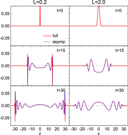
Figure 1. Spatial variations of u at different times.
Download figure:
Standard image High-resolution imageThe initial disturbance generates two groups of waves propagating in opposite directions. The waves propagating upward are described by positive k, and those propagating downward are described by negative k. Our interest is mainly in the upwardly propagating waves with  . Note that k for any wave packet can be inferred from the inverse of the distance between the neighboring zeros in the figure. The figure clearly shows that in each group, larger-k (and hence higher-ω) wave packets keep ahead of smaller-k (and hence lower-ω) packets. This kind of dispersion arises from the fact that the distance of travel, z, is proportional to vg for a fixed t and the magnitude of vg increases with that of k, as can be seen from Equation (29), which can be solved for k as in

The plots of velocity fluctuations versus time shown in Figure 2 confirm that higher-ω wave packets arrive at a remote region earlier than lower-ω wave packets. Note that ω for a wave packet can be inferred from the inverse of the time between the neighboring zeros in the figure. As mentioned above, higher-ω wave packets are generated by the larger-k components of the initial perturbation and have higher group speeds than lower-ω waves that are generated by the smaller-k components of the initial perturbation. As a consequence, the oscillation frequency changes with time from high to low values at a fixed point. In fact, ω asymptotically approaches 1, so that after a long time, the velocity oscillates with a frequency of 1, as can seen from the explicit expression of ω:

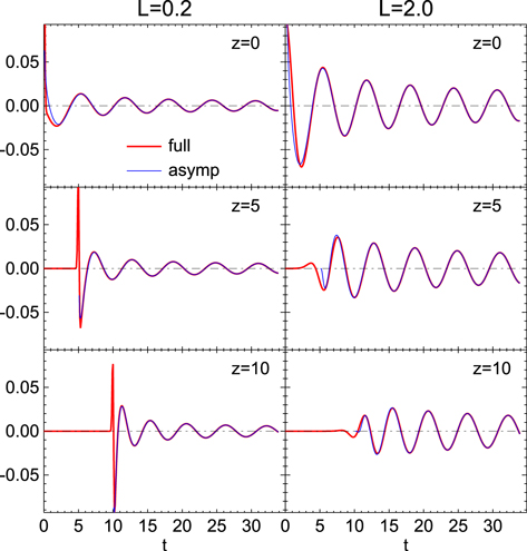
Figure 2. Temporal variations of velocity fluctuation u at different distances from the origin.
Download figure:
Standard image High-resolution imageUsing the temporal variations of velocity at two different positions shown in the top left panel of Figure 3, we have investigated the variations of oscillation frequency ω, group velocity vg, and phase speed vp over time. The oscillation frequency ω was inferred from the time interval between two successive moments of zero velocity by regarding each interval as half the period at that moment. The measured frequency is found to drift from high to low with time asymptotically approaching 1, as mentioned above. This measured frequency was used to calculate the group speed vg and phase speed vp at each moment. The group speed was also independently estimated using the distance and time of travel from the origin. These two different methods produce the same results for the group speed, confirming the notion that the wave packet propagates at the group speed, with higher-frequency wave packets propagating faster than lower-frequency wave packets. The phase speed was also independently inferred from the differences between the moments of zero velocity between the two different altitudes at specific times. The phase speed determined in this way is in good agreement with the one calculated from the measured ω. Unsurprisingly, the figure clearly illustrates that vg is smaller than 1 and inversely proportional to t while vp is larger than 1 and proportional to t, satisfying  .
.
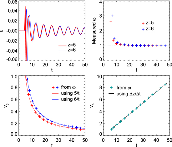
Figure 3. Top left: the temporal variation of u at two different heights in the case in which L = 0.2. Top right: temporal variation of the measured ω. Bottom left: vg inferred from the measured ω and those inferred from the travel distance z and time t. Bottom right: vp inferred from the measured ω and those inferred from the two different heights.
Download figure:
Standard image High-resolution imageThe time-distance maps of u in Figure 4 further illustrate the dispersive nature of acoustic waves that are modified by the gravitationally stratified medium. Note that a wave packet of a specific wavenumber k and its corresponding frequency ω propagate along the curve of  in
in  space where vg is given as a function of k as in Equation (29). It can be seen from the figure that the wave packet keeps the same pattern along each curve. The maps indicate that high-ω wave packets quickly escape from the source region compared to the escape time of the low-ω packets. A remote region away from the source region first experiences the arrival of high-frequency waves, but these waves pass through this region in a short time. The region then experiences the arrival of lower-frequency waves. The waves with frequencies close to one come very much later and move very slowly so that they "linger" there for a quite long time once they arrive. Thus, what we see is that the three-minute oscillations are not standing waves, but represent packets of gravity-modified small-k acoustic waves that propagate with a group velocity that is much slower than the speed of sound.
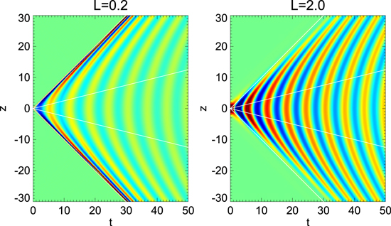
Figure 4. Time–distance plot of u for the two models. Red represents upward motion, and blue, downward motion. Overplotted are the curves of  .
.
Download figure:
Standard image High-resolution imageFigure 5 reveals that the theoretical power spectrum satisfactorily matches the observed ones. The theoretical power spectrum was constructed from the time variation of velocity for t = 10 through 80 at z = 10 in the case of L = 2.0 as shown in Figure 2. The sampling interval and coverage range were chosen so as to match those of the observations to which the calculations are compared. The theoretical power spectrum has peaks just above the cutoff frequency, where  is about 1.02. The spectrum has a sharp cut at the cutoff frequency, and a high frequency wing that decreases with frequency. The internetwork data were taken from Figure 10 of Chae et al. (2013) and the sunspot data from Figure 10 from Cho et al. (2015). The data are of a 30 minute duration, with a sampling rate of 20 s, and were used to compute the power spectra utilizing the Lomb–Scargle method. Each power spectrum was normalized to the primary peak, and the cutoff frequency was inferred from the frequency of the primary peak. As far as the primary peak is concerned, we find a good agreement between the theoretical power spectrum and the observations.
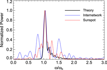
Figure 5. Comparison of the power spectra of velocity oscillations between our theory and observations. The internetwork oscillation data were taken from Figure 10 of Chae et al. (2013) and the sunspot oscillation data from Figure 9 of Cho et al. (2015).
Download figure:
Standard image High-resolution imageIt is worthwhile to compare the values of the peak periods, or the corresponding cutoff frequencies, between the different regions. We have obtained a primary peak period of 3.2 minutes for the internetwork oscillations and 2.6 minutes for the sunspot oscillations, which correspond to  and 0.039 rad s−1, respectively. According to our theory, the above regional dependence of the oscillation period can be attributed to the difference in the temperature between the source regions. Choosing g = 0.274 km s−2 and
  , we obtain a sound speed for the source region of
  7.1 and 5.8 km s−1, and the temperature of the same regions
  5160 and 3440 K, respectively, for the internetwork area and the sunspot area, where we have chosen a mean molecular weight of
  .
.
4. WAVE ENERGY AND FLUX
Figure 6 compares the temporal variations of u,  , and
, and  at a fixed point. At the earliest moments, when the high-frequency wave packets pass through the point,
  varies in phase with, and has the same amplitude as u, while the displacement ξ has a small amplitude. Thus, there is an approximate equipartition between kinetic energy and intrinsic energy, and the ratio of energy flux f to the total energy
  is as high as 1. At later times, when low-frequency wave packets arrive at the point, however,
  comes to be out of phase with, and have a smaller amplitude than, u. In this case, energy equipartition holds between kinetic energy and potential energy, and the ratio
  becomes lower than 1.

Figure 6. Top: temporal variations of velocity u, pressure ζ, displacement ξ (top), total energy density  , and energy flux f (bottom) at a fixed point z = 10.
Download figure:
Standard image High-resolution imageBy making use of Equations (30)–(33), we can derive the following expressions for the energy densities averaged over one period of time ( ) at a fixed point


which leads to the equipartition relationship  . Moreover, in the wave packets having
  (the limit of ordinary acoustic waves propagating in a uniform medium),
  and
and  . By contrast, in the wave packets having
  (the limit of natural frequency oscillations), we have
  for
for  .
.
From Equations (30) and (33), we can also derive the expression for the energy flux averaged over one period of time ( )
)

which supports the well-known relationship that energy flux is given by the product of total energy density  and group velocity vg. Note that the pressure fluctuations in Equation (33) consist of two parts: one part is in phase with the velocity fluctuations u and the other part is out of phase with u and in phase with the displacement ξ. Only the first part contributes to the transport of energy, and its contribution is proportional to k and hence vg. Therefore, when this part dominates (
 ), the group speed is close to the sound speed, but when it is insignificant (
 ), the group speed is much lower than the sound speed. In this way, the group speed directly reflects the cross-correlation between velocity fluctuations and pressure fluctuations.
It is worthwhile to examine how different kinds of energy change with time in the source region defined by the disturbed region and the region surrounding it. This is particularly important to understand the decay of velocity amplitude with time, as is well-known from previous studies, and in understanding the conditions for the persistence of the free oscillations. We have chosen the spatial range ![$[-10,10]$](https://content.cld.iop.org/journals/0004-637X/808/2/118/revision1/apj516741ieqn114.gif) to define the source region. Figure 7 shows the kinetic energy
to define the source region. Figure 7 shows the kinetic energy  , the intrinsic energy
  , the potential energy
  , and the total energy
  as a function of time, where the integrations were carried out over
 ![$[-10,10]$](https://content.cld.iop.org/journals/0004-637X/808/2/118/revision1/apj516741ieqn119.gif) using the full solutions for Equations (19)–(22). The figure also shows the total amount of energy lost by the transport of energy across the two boundaries
using the full solutions for Equations (19)–(22). The figure also shows the total amount of energy lost by the transport of energy across the two boundaries  , as given by
  .
.

Figure 7. Time variations of E, K, P, U, and F for the two cases. The spatial integrations were performed over the range [−10, 10].
Download figure:
Standard image High-resolution imageNote that for  , the disturbance is confined to the source region so that the integrations over
 ![$[-10,10]$](https://content.cld.iop.org/journals/0004-637X/808/2/118/revision1/apj516741ieqn123.gif) are equivalent to the integrations over the range
are equivalent to the integrations over the range  . Therefore for
  , by applying Parseval's theorem, we can obtain K, P, and U expressed as the integrations of power over the spectral domain


from which we can easily derive the relationships

which leads to energy equipartition  , and the constancy of total energy over time and

Figure 7 shows that the relative importance of P and U depends on L, the length scale of the disturbed region. When L is smaller than 1, P is more important, and when L is bigger than 1, U is more important. When averaged over one period of time, half of the total energy is in kinetic energy, and the dominant portion of the other half is in potential energy, and the rest is in intrinsic energy.
More importantly, Figure 7 indicates that the total energy E of the source region decreases with time for  , because energy is transported out of the region by the waves. The kinetic energy K decreases with time as well, which is a consequence of energy transport. This energy transport naturally accounts for the decay of velocity amplitude at a specific height that has been reported by previous studies and is seen in our study. In this aspect, we make two points. First, the sum of E and F does not change with time. This means that the total energy of the infinite volume is conserved, and the decay of velocity amplitude at a given height has nothing to do with any irreversible dissipative process. Second, E decreases more rapidly to zero in the case of L = 0.2, than in the case of L = 2.0. This means that the source region for
  is efficient in emitting mechanical energy, while the one of
  is inefficient in emitting it and is instead efficient in keeping it. In this regard, the source region of
  acts like a leaky cavity for mechanical energy. This low efficiency energy transport is closely related to the low group speed for small-k waves and is responsible for the persistence of natural frequency oscillations not only inside, but also outside the source region. The gravitationally stratified medium can maintain long-lasting oscillations and waves with frequency near the cutoff frequency because of the inefficiency of energy transport.
5. WAVES GENERATED BY A SERIES OF IMPULSIVE DISTURBANCES
The solar observations indicate that three-minute chromospheric oscillations exist always and everywhere, not being localized in time and space. This characteristic suggests that the chromospheric oscillations are driven constantly either by continuous driving or by the continual occurrence of impulsive disturbances. By generalizing the solution, and by applying the superposition principle, we construct a more generalized solution

to describe the velocity of the waves driven by multiple disturbances, each of which is characterized by the set of parameters: ti, zi, Li, and u0i. Here H is the Heaviside step function. The solutions for ζ, η, and ξ can be obtained in the same way.
Figure 8 illustrates the waves generated by a series of repeated disturbances. For simplicity, we have kept zi = 0, Li = 2,  , and we specify the multiple events by their instant of occurrence:
  for
for  with T = 23.3. If we use the dimensional values Hv = 230 km, and c = 7.2 km s−1 mentioned in the previous section, we obtain Li = 460 km,
  km s−1, and T = 12.4 minutes. The figure indicates that a finite amount of energy is being continually injected into the acoustic waves at every instance of time ti, which can maintain the free atmospheric oscillations despite the energy loss due to the outward propagation through the boundaries. Note also that the amount of injected energy varies little from event to event, since the atmosphere is not in hydrostatic equilibrium any longer at
  , unlike at t = 0. The amount of injected energy depends not only the parameters above, but also the pre-existing fluctuations of the medium at each instance of energy injection.

Figure 8. Top: time variations of the energy injection rate and the total energy for the waves that are generated by a series of impulsive events occurring at uniformly spaced time intervals. Here E is the energy of the region ![$[-10,10]$](https://content.cld.iop.org/journals/0004-637X/808/2/118/revision1/apj516741ieqn136.gif) and F is the energy that has propagated out of this region.
and F is the energy that has propagated out of this region.  is equal to the energy of the infinite region
  . Bottom: time variation of velocity at z = 10 and its power spectrum.
Download figure:
Standard image High-resolution image
The time variation of velocity presented in this figure mimics the observed ones like Figure 9 of Cho et al. (2015) in that the oscillations exist at all the times, and the amplitude of the oscillations changes with time. Note that this similarity could have been obtained simply by taking into account a series of similar impulsive events. If the moments of occurrence and the other parameters would be stochastic, then time variation of the constructed velocity could be made to look more realistic. The power spectrum shown in the figure indicates that the peak occurs at a frequency just above the cutoff frequency, as in the case of the waves generated by a single impulsive event (see Figure 5), even though the precise value of the peak frequency varies a little with the set of the parameters used for the peak's construction.
The theoretical waves generated by the series of impulsive events can be quantitatively compared with the observed waves in the solar chromosphere. The average rate of energy injection is given by

in dimensionless units or

in dimensional units. Note that P has physical units of erg cm−2 s−1, which can be directly compared with the observable energy flux of acoustic waves in the solar atmosphere. The recent observations indicate that the flux of acoustic waves at frequencies above  is 2–
is 2– erg cm−2 s−1 (e.g., Bello González et al. 2010a, 2010b). If we choose L = 2, T = 25, and u0 = 0.1, the theoretical rate of energy injection in Equation (46) can match these observational values with the values of
  and c at the atmospheric height of 300–400 km in the FAL model of the solar atmosphere. This supports the possibility that the impulsive disturbances in the upper photosphere can drive the three-minute free oscillations.
6. SUMMARY AND DISCUSSION
We have shown theoretically that the initial disturbance of a region in a gravitationally stratified medium produces two groups of gravity-modified acoustic waves propagating in opposite directions that have frequencies above the cutoff frequency  . These waves are dispersive; large-k perturbations produce high-frequency waves that have group speeds as high as the sound speed, and small-k perturbations produce low-frequency waves that have group speeds much lower than the sound speed. Thus, the high-frequency waves quickly escape out of the source region, but the waves with low frequencies close to
  linger around the source region for a long time. Therefore, it is these latter waves that are identified as the three-minute oscillations observed in the chromospheres of the internetwork regions of the quiet Sun and the umbrae of sunspots. We find that the persistence of high amplitude three-minute oscillations can be explained by a series of impulsive disturbances on length scales larger than
  . These processes can continuously inject sufficient energy to maintain the acoustic waves of frequencies close to
  .
.
In several respects, the results of our study further clarify the nature and origin of the three-minute chromospheric oscillations. Our study is in line with the previous studies that presented a picture of a resonant response or free atmospheric oscillations (Fleck & Schmitz 1991; Kalkofen et al. 1994; Sutmann & Ulmschneider 1995; Sutmann et al. 1998) in that we attribute the three-minute oscillations to the intrinsic properties of the medium itself, neither to the resonant cavity surrounded by two barriers (Leibacher & Stein 1981) nor to the driving at frequencies  . There are, however, more features noticeable from our study. First, our results suggest that the three-minute oscillations have the nature of propagating acoustic waves at frequencies above
  . These waves are subject to the effects of gravity, and are characterized by small wavenumbers
  . This non-zero power at
  is important because a disturbance with
  can propagate. The waves can transport energy with group speeds much lower than the sound speed. This propagating and energy-transporting nature explains the decay of velocity amplitude with time reported from these studies. Second, for a similar reason, the three-minute oscillations observed for a finite time interval are not a resonant phenomena in the common physical sense because the peak power of the chromospheric oscillations occurs mostly at a frequency higher than
  , not exactly at it. This deviation arises because a disturbance has non-zero power at
  . The peak power would occur exactly at
  only when all the power of oscillations would be concentrated at k = 0 (that is, disturbance of infinite size) so that the whole atmosphere would oscillate together. This situation occurs in the limit of
  when all the disturbances with
  have moved away to infinity. The oscillations at frequency
  only are very special in this regard, and are not realistic. Third, our study suggests that the persistence of the three-minute oscillations originates from the physical processes that can supply energy to waves of frequencies a little above
  and wavenumbers satisfying the condition
  . The velocity impulse with the δ-function shape considered by Lamb (1909) and Kalkofen et al. (1994) is not an optimal process of origin for the three-minute oscillations, since the energy is evenly distributed over the k space and the fraction of energy at
  is small. Instead we have adopted the velocity impulse of Gaussian function with a correlation length L. The larger L is, the larger the fraction of energy with
  is. Our study finds that the velocity impulse with
  can supply the energy at such wavenumbers necessary for the three-minute oscillations.
Based on our study, we now attempt to interpret some results from the previous studies. Specifically, we examine the driving of the three-minute chromospheric oscillations by the five-minute oscillations. Fleck & Schmitz (1991) first demonstrated that three-minute oscillations appear in the atmosphere when its lower boundary is driven by a sinusoidal piston motion of five-minute period. This phenomenon cannot be explained by the picture of a chromospheric cavity. It is also apparently in contradiction to the concept of the acoustic cutoff. We can interpret this phenomenon in terms of the dispersive nature of the medium. We conjecture that this phenomenon takes place not because the piston moves continuously with five-minute period, but because the piston sets up motions suddenly from the initial equilibrium. Because of the discontinuous time-derivative of velocity at time t = 0, the driving motion involves high-frequency velocity disturbances with  in addition to the driving frequency. These high-frequency components propagate; the highest frequency component propagates at the sound speed, and the lower frequency components propagate at slower speeds. The lowest frequency components with
  survive for the longest time, which can then be identified as the chromospheric oscillation. In that the driving by the initiation of the five-minute oscillation motion at the lower boundary is impulsive, and the disturbances of different frequencies propagate at different speeds, this driving is similar to the driving by a localized velocity impulse considered in the previous studies (Lamb 1909; Kalkofen et al. 1994) and in the current study. The driving by a sinusoidal pulse of velocity (Sutmann & Ulmschneider 1995; Sutmann et al. 1998) is also similar in this regard. This kind of driving is equivalent to two velocity impulses separated by a finite time. The point is that the results of our study are compatible with, and help one understand, the results from the previous studies.
Now we address to the question of what kind of processes can supply enough energy to the atmosphere to maintain the three-minute oscillations. Our study suggests that the processes have to satisfy two necessary conditions. First, they should be able to inject enough energy at wavenumbers satisfying  or at frequencies above
  . Second, the energy injection should occur either continuously or repeatedly. The driving by a continuous sinusoidal motion of a lower frequency
  like the five-minute oscillations does not satisfy these conditions. The impulsive start of the driving from the initial static equilibrium injects energy at frequencies above
  , but the amount of the energy at such frequencies is very small compared with the energy of the driving motion itself. Moreover, the energy injection occurs only once. The driving by a sinusoidal pulse is a little better since it is equivalent to two impulses, but is subject to a similar problem.
Do any of the physical processes proposed so far satisfy the conditions above? The supply of high frequency acoustic power through the bottom of the photosphere is one plausible process. Sutmann et al. (1998) theoretically demonstrated that the excitation by a wavetrain of pulses that are continually generated and have randomly chosen amplitudes and frequencies can permanently maintain the free atmospheric oscillations. This idea can explain why Carlsson & Stein (1997) were successful in simulating the occurrence of the three-minute chromospheric oscillations using the velocities measured from a photospheric spectral line as a function of time, considering that the real photospheric motion in the photosphere may contain high frequency components generated below the photosphere. The generation of the high frequency acoustic waves by turbulent convection may be important in this regard. The recent sophisticated and realistic calculations of Fawzy & Musielak (2012) indicate that turbulent convection can continuously generate waves that have enough power at high frequencies above the acoustic cutoff frequency in the photosphere of late type stars. Interestingly, in this study most of the acoustic flux power at the photospheric level occurs over a broad range of frequencies notably above the acoustic cutoff (which is about 5 mHz) covering up to 60 mHz in the solar-like G0V star, but the power of the oscillations in the middle chromosphere is sharply peaked at 8 mHz, a little above the cutoff frequency. This behavior cannot be understood with a linear theory alone, but can be understood when nonlinear effects such as shock merging (Kalkofen et al. 1994; Theurer et al. 1997) are taken into account. Theurer et al. (1997) demonstrated that the merging of high frequency shock waves generated by a sinusoidal motion of period shorter than 30 s in the photosphere leads to the generation of three-minute oscillations in the chromosphere.
Another possible process is a series of velocity impulsive events with correlation a length scale bigger than twice the pressure scale height we proposed. What specific physical processes in the solar atmosphere would be in this category? One is acoustic events. Motivated by Stebbins & Goode's (1987) finding of unexpected behavior of phase changes of photospheric five-minute oscillations with height, Goode et al. (1992) theoretically investigated the effect of localized excitation below the photosphere and concluded that many of the five-minute acoustic modes in the photosphere could be excited by isolated expansive events centered about 200 km beneath the base of the photosphere and that the seismic events last about five minutes. These events are called either acoustic events or seismic events. These events can be one cause of the initial disturbance we supposed in the present work.
The idea of acoustic events dates back to Lamb (1909) who considered the effect of the δ-function like disturbance on the atmosphere. By re-analyzing the data of Stebbins & Goode (1987), Restaino et al. (1993) identified acoustic events by the events showing large mechanical flux and found oscillatory wakes in them in agreement with the events modeled by Goode et al. (1992). Subsequent studies showed that these events occur preferentially in the dark, intergranular lanes, suggesting that the disturbance caused by the rapid cooling in the surface, which generates acoustic waves (Rimmele et al. 1995) and they pump power into the resonant modes of vibrations of the Sun (Goode et al. 1998). Even though Goode et al.'s (1992) study was not aimed at explaining the three-minute chromospheric oscillations, all of their simulations display three-minute oscillations in the chromosphere even though the durations of the acoustic events are longer. In fact, observations have supported the tendency for acoustic events in the photosphere to be correlated with the bright Ca ii grains, which are known to be chromospheric events of three-minute oscillations (Hoekzema et al. 2002; Cadavid et al. 2003; Kamio & Kurokawa 2006).
The other candidate for the excitation process is the events of small-scale reconnection in the photosphere and low chromosphere. The existence of such a possible connection was already indicated by Yang et al. (2014), who reported that an Ellerman bomb, which is thought to be an event of magnetic reconnection, generates a series of shock waves that drive a surge. This kind of event may be less frequent than the acoustic events, but may be worthy of further investigation.
7. CONCLUSION
We conclude our study by providing the answers to the questions raised in the introduction. The atmosphere excited by the lower boundary motion of five-minute oscillations displays three-minute free oscillations because the driving starts from the static initial state, which involves the injection of a small amount of power at frequencies above the acoustic cutoff frequency. The resulting free oscillations are propagating acoustic waves that are dispersive in nature. The amplitude of the velocity at any height decays with time because the energy is being continuously transported out of the region. The higher frequency waves first move out of the region, and gradually the lower frequency waves move away, and the waves with the acoustic cutoff frequency survive permanently but their power is too small to be significant. In order to permanently maintain the three-minute free oscillations, there should be processes that can inject enough energy at frequencies just above  or at spatial scales larger than twice the pressure scale height. Moreover, the processes have to occur repetitively so that energy can be continually re-supplied. There are two main process satisfying these conditions: one is the generation of high frequency acoustic waves by turbulent convection below the photosphere and the other is a series of velocity impulses of correlation length
  such as the acoustic events occurring in the upper photosphere. For realistic results, the effects of temperature structure and nonlinear processes should be properly taken into account, which is beyond the scope of the present work, but is what the current sophisticated numerical simulations usually do (e.g., Fawzy & Musielak 2012).
The work of J.C. was supported by the National Research Foundation of Korea (NRF—2012 R1A2A1A 03670387). P.R.G. gratefully acknowledges the support of the Air Force Office of Scientific Research grant FA9550-15-1-0322, the National Science Foundation grant AGS-1250818, and the National Aeronautics and Space Administration grant NNX13AG14G. We are grateful to K. Cho for providing with us with the data originally used for Figure 9 of Cho et al. (2015).