


ABSTRACT
Langmuir turbulence excited by electron flows in solar wind plasmas is studied on the basis of numerical simulations. In particular, nonlinear wave decay processes involving ion-sound (IS) waves are considered in order to understand their dependence on external long-wavelength plasma density fluctuations. In the presence of inhomogeneities, it is shown that the decay processes are localized in space and, due to the differences between the group velocities of Langmuir and IS waves, their duration is limited so that a full nonlinear saturation cannot be achieved. The reflection and the scattering of Langmuir wave packets on the ambient and randomly varying density fluctuations lead to crucial effects impacting the development of the IS wave spectrum. Notably, beatings between forward propagating Langmuir waves and reflected ones result in the parametric generation of waves of noticeable amplitudes and in the amplification of IS waves. These processes, repeated at different space locations, form a series of cascades of wave energy transfer, similar to those studied in the frame of weak turbulence theory. The dynamics of such a cascading mechanism and its influence on the acceleration of the most energetic part of the electron beam are studied. Finally, the role of the decay processes in the shaping of the profiles of the Langmuir wave packets is discussed, and the waveforms calculated are compared with those observed recently on board the spacecraft Solar TErrestrial RElations Observatory and WIND.
Export citation and abstract BibTeX RIS
1. INTRODUCTION
Direct observations of Langmuir waves in the solar wind and, in particular, in the source regions of type III solar bursts (e.g., Gurnett et al. 1981, 1992; Kellogg 1986; Kellogg et al. 1992, 2009; Ergun et al. 1998; Nulsen et al. 2007; Malaspina et al. 2010; Hess et al. 2011; Graham & Cairns 2013, and references therein) and in the Earth's foreshock (e.g., Bale et al. 1996, 2000; Souček et al. 2005) show poor agreement with the predictions of the theory of Langmuir turbulence excited by electron beams in homogeneous plasmas (e.g., Vedenov et al. 1961, 1967; Musher et al. 1995). Moreover, many physical aspects revealed by the observations could not be described by analytical studies considering plasmas with simple density gradients or large density fluctuations (e.g., Breǐzman & Ruytov 1970; Ryutov 1970). Thus, it is worth solving this conflict by taking into account the important role of plasma density irregularities in such plasmas and performing adequate numerical simulations, using kinetic or fluid approaches (e.g., Kontar & Pecseli 2002; Krafft et al. 2013). On this basis it was shown on one hand that monotonic density gradients or randomly fluctuating density inhomogeneities are able to strongly modify the development and even the nature of the wave–particle and the wave–wave interactions at work and that on the other hand they can prevent the appearance of such nonlinear processes as wave decay, induced scattering, or modulation instability (but generally not beam quasilinear diffusion), whose descriptions are mostly based on theories developed in the frame of homogeneous plasmas (e.g., Zakharov 1972; Galeev et al. 1977; Rubenchik & Shapiro 1993). Note that the low-frequency oscillations of both the plasma density and the ambient magnetic field can in principle significantly influence on the development of the beam instability and the waves' dynamics. However, since the solar wind magnetic field is weak (the ratio between the electron cyclotron and plasma frequencies satisfies ωc/ωp ≲ 10−2) and its effect on the dispersion of the plasma waves is negligible, one can assume that the fluctuating density irregularities only can have a significant impact on the Langmuir waves' and beams' dynamics. Unfortunately, only few direct measurements in the solar wind of such density fluctuations are available up to now, which can be used to determine their spectral properties as well as their average level (e.g., Celnikier et al. 1983, 1987; Kellogg et al. 1999; see also Malaspina et al. 2010).
One of the first simultaneous observations in the solar wind of long-wavelength density fluctuations (possibly ion sound (IS) waves) and intense Langmuir waves excited by electron beams associated with type III bursts was presented by Lin et al. (1986); they were interpreted as being due to nonlinear processes involving wave–wave interactions and in particular to Langmuir wave decay. Evidence or suspicion for three-waves' interactions in the source regions of type III solar radio bursts or in front of planetary bow shocks were reported in numerous papers; for example, the observations of waveforms in front of the Jovian bow shock were interpreted as beatings of Langmuir waves due to their interactions with IS waves or density fluctuations (Gurnett et al. 1981; Cairns & Robinson 1992). More recent evidence for three-waves' interactions involving Langmuir waves in the electron foreshock region as well as in the source regions of type III solar bursts was reported by several authors (e.g., Lin et al. 1981, 1986; Robinson & Newman 1991; Gurnett et al. 1993; Hospodarsky et al. 1994; Hospodarsky & Gurnett 1995; Bale et al. 1996; Thejappa et al. 2003; Souček et al. 2005; Henri et al. 2009; Graham & Cairns 2013, and references therein). Meanwhile, observations of electron fluxes or beams in the solar wind near the Earth's orbit were presented in other works (e.g., Lin et al. 1981; Ergun et al. 1998).
Recent studies of the wave activity measured on board satellites such as POLAR, ULYSSES, WIND, and the Solar TErrestrial RElations Observatory (STEREO) have revealed many new features of the Langmuir turbulence in much greater detail. For example, Langmuir wave decays during type III radio bursts are presented for 14 events observed by STEREO (Bougeret et al. 2008), where all wave packets were registered within a duration τ ≃ 130 ms; the authors (Henri et al. 2009) argue that the threshold in the solar wind (Lin et al. 1986) of the decay instability of a Langmuir wave  into another Langmuir wave
  and an IS wave
  (i.e.,
  hereafter called Langmuir electrostatic decay) is significantly exceeded. Moreover, Graham & Cairns (2013) show that around 40% of the Langmuir waveforms observed by STEREO during type III solar radio bursts can be consistent with the occurrence of such decays, and even with one or more of their cascades. It is interesting to note here that the Langmuir wave profiles and spectra obtained using the INTERBALL-2 satellite's data (Burinskaya et al. 2004) in the inner regions of the Earth's magnetosphere are very similar to those observed in the solar wind type III regions or the foreshock; the explanation proposed by the authors is based on the weak turbulence theory of beam-excited Langmuir waves' scattering on the external IS turbulence.
In the papers reporting observations of Langmuir waves' decays in the solar wind, few arguments in favor of such nonlinear processes are mainly used (e.g., Lin et al. 1981, 1986; Robinson et al. 1993; Cairns & Robinson 1995; Hospodarsky & Gurnett 1995; Kellogg et al. 1999; Henri et al. 2009; Graham & Cairns 2013 and references therein): (1) the existence of a double peaked structure in the Langmuir wave spectrum; (2) the simultaneous observation of intense Langmuir waves and IS waves or plasma density oscillations. In some cases, the frequencies of the observed IS waves fit well with the theoretical predictions of electrostatic decay based on beam and plasma measurements; (3) the estimate of the waves' intensities showing that the threshold of the Langmuir parametric instability in homogeneous plasmas is exceeded; (4) the tendency of the Langmuir waveforms observed to clump and burst, which exhibit modulation frequencies consistent with beatings between mother and daughter Langmuir waves. Usually these topics are not invoked all together simultaneously; moreover, in some cases, no signature of low-frequency waves could be detected. Note finally that in order to conclusively identify an electrostatic decay, one should also verify the resonance conditions by a spectral analysis, the time occurrence of the waves by a wavelet analysis, and the phase correlations between the waves by a bicoherence analysis (e.g., Dudok de Wit & Krasnoselskikh 1995; Thejappa et al. 2013).
When the threshold of the parametric instability is exceeded, intense Langmuir waves can decay into daughter waves according to the channel  , producing backscattered Langmuir waves
  and IS waves
  propagating in the same direction as the parent waves (in a one-dimensional (1D) description). If the
  waves carry enough energy, a possible secondary decay cascade can occur according to the channel
  producing in turn Langmuir waves
  propagating in the same direction as the mother waves
  and IS waves
  propagating in the inverse direction. In principle, more cascades can occur until the decays become prohibited due to kinematic effects. The process
  allows the transfer of part of the wave energy from larger k-space regions to smaller ones, and in particular from regions where the beam resonantly excites waves (beam-driven mother waves) to regions (i) where such resonant phenomena are not possible (nonresonant domains where k < 0, for example) or (ii) where the waves can resonantly damp and consequently release energy to beam particles and possibly accelerate them (when k < kb, where kb = ωp/vb and vb is the beam initial velocity). When the instability threshold is exceeded, the dynamics of the decay process depends notably on the energy of the parent Langmuir waves and on the efficiency of transferring it to the daughter waves, effects which are both influenced by the average level of randomly varying density fluctuations (and also by their wavelengths). In turn, decay processes can significantly influence the features of the Langmuir waveforms eventually observed and contribute to the shape of their modulations and accentuate their tendency to clump. Moreover the excitation of large-amplitude backscattered Langmuir waves may also lead to the appearance of transverse electromagnetic waves
  near 2ωp through the coalescence of two Langmuir waves, i.e., according to the channel
  (ωp is the electron plasma frequency). This process is believed to be a first step for the generation of type III radio emissions at 2ωp; those can also be produced when a Langmuir wave decays in a transverse electromagnetic wave at ωp and a low-frequency wave. Note that in the present study wave decay involving electromagnetic waves is not considered.
For all the reasons invoked above, it is essential to study Langmuir decay in solar wind plasmas using numerical simulations, especially because only a few analytical works exist dealing with inhomogeneous plasmas (e.g., Breǐzman & Ruytov 1970; Ryutov 1970). In this view, several numerical simulations have been carried out in order to study the dynamics of wave decay in unmagnetized or weakly magnetized plasmas. Most of them were performed in the frame of the weak turbulence kinetic theory (e.g., Ziebell et al. 2001; Li et al. 2003; Henri et al. 2010), considering homogeneous plasmas and more rarely plasmas with inhomogeneities and in this latter case mainly in the form of monotonic gradients (e.g., Kontar & Pecseli 2002). Particle-in-cell (PIC) codes (e.g., Huang & Huang 2008) or Vlasov codes (e.g., Umeda & Ito 2008; Henri et al. 2010) have been used. Other simulations were performed in the frame of a fluid description using the Zakharov equations (e.g., Gibson et al. 1995). Among all these works, some were applied to study Langmuir wave decay in solar wind plasmas and in particular in the Earth's foreshock or in the source regions of type III solar bursts. Moreover, some were devoted to investigating not only wave decay but also other processes such as scattering off thermal ions, for example (see Cairns 2000, and references therein).
The present paper focuses on the problem of Langmuir wave decay in solar wind plasmas typical of type III bursts' source regions near 1 AU where, as mentioned above, several observations report that such process can commonly occur; moreover, it is likely one of the most important mechanisms at work in these conditions. In such plasmas, randomly varying density fluctuations exist with average levels Δn reaching up to several percents of the background plasma density (Celnikier et al. 1983, 1987; Kellogg et al. 1999); therefore, wave decay generally occurs simultaneously with other coupling effects between the fields and the density inhomogeneities, such as reflection, scattering, or refraction processes. For example, reflection phenomena on plasma irregularities can lead to the appearance of reflected waves of noticeable amplitudes which can couple to the beam-driven waves. In this case, electrostatic decay is less probable in plasmas with large average levels of density fluctuations (Δn ≳ 0.03) than resonant wave–wave coupling, for which the resonance conditions are the same and the beatings between Langmuir waves also produce IS waves. In quasi-homogeneous plasmas, i.e., plasmas with density fluctuations of the order of or lower than Δn ≃ 0.001–0.005, where reflection effects are weak, "pure" electrostatic decay with daughter waves actually rising from the thermal noise can occur. Moreover, wave reflection on the gradients of the density fluctuations lead, near the reflection points of the density humps and wells, to wave energy focusing and to the appearance of short wave turbulence.
Thus, the aim of the paper is to understand what is the influence of plasma density inhomogeneities on the wave decay processes, that is, if they can favor or prevent their occurrence, and under what conditions. Note that at least two points will complicate the analysis of the simulation results and their comparison with theoretical works: (i) analytical studies were performed mainly for monochromatic waves (e.g., Sagdeev & Galeev 1969; Zakharov et al. 1985), whereas our simulations involve broad wave packets; (ii) homogeneous or quasi-homogeneous plasmas were mostly considered even if some works include inhomogeneous plasmas with simple gradients or random oscillations (Breǐzman & Ruytov 1970; Ryutov 1970; Escande & de Genouillac 1978), whereas we take into account self-consistently randomly varying density inhomogeneities. Let us mention finally that in the frame of our theoretical model (see below) and according to the typical ratios of electron to ion temperatures in the solar wind, electrostatic decay overcomes the process of scattering off thermal ions (see also, e.g., Cairns 2000). Moreover, phenomena as modulational instability or collapse should not occur for our parameters due to their characteristic ranges of wavenumbers and high-frequency wave energy densities (Zakharov et al. 1985).
The simulation results are provided by a numerical code based on a Hamiltonian model (Krafft et al. 2013; Volokitin et al. 2013) where the self-consistent resonant interactions between beam electrons and Langmuir waves are described in a plasma involving density fluctuations for conditions relevant to solar type III observations at 1 AU (e.g., Ergun et al. 1998). Using the Zakharov's equations with an additional term representing the electron beam, the model takes into account strong preexisting and randomly varying density inhomogeneities and includes the low-frequency plasma response. The beam is modeled using a PIC description. Ponderomotive force effects are included, even if the density fluctuations do not result from strong turbulence phenomena. Contrary to the usual PIC approach where great numbers of particles are used to minimize the numerical noise, our model consists of dividing the electron distribution into two populations: (i) the bulk particles, forming the ambient plasma, which support the waves' propagation but do not interact resonantly with them; and (ii) the resonant beam electrons which exchange significant amounts of momentum and energy with the waves, and whose motion is solved by the Newton equations (e.g., O'Neil et al. 1971; Volokitin & Krafft 2004; Zaslavsky et al. 2006). One of the advantages of this approach is to greatly reduce the number of particles used in the simulations and to solve their dynamics over long periods of time (e.g., Volokitin & Krafft 2012).
2. SUMMARY OF THE THEORETICAL MODEL
Let us briefly summarize the theoretical model used and described in more detail in previous papers (Krafft et al. 2013; Volokitin et al. 2013). The interaction of Langmuir waves' packets with an electron beam in an inhomogeneous solar wind plasma can be studied in 1D geometry as most of the observed Langmuir wavefields are polarized along magnetic field lines (Ergun et al. 2008). The background plasma of density n0 is described through the dielectric constant using linear theory, whereas only the resonant beam particles, of density nb ≪ n0, interact with the electric Langmuir fields through the Landau resonance (e.g., O'Neil et al. 1971; Volokitin & Krafft 2004; Zaslavsky et al. 2006).
The full Hamiltonian of the waves-particles-plasma system can be written as  , where
  is the Hamiltonian corresponding to the Zakharov equations (Zakharov 1972) without the beam source term
and  takes into account the kinetic energy of the resonant particles and their energy of interaction with the waves

The electric field is  where
where  is the slowly varying field envelope,
  ; Ek is the Fourier component of E; z is the space coordinate and k is the wave vector;
  is the Langmuir wave frequency; ωp and λD are the electron plasma frequency and Debye length; δn is the ion density perturbation; me and mi are the electron and ion masses, u is the velocity of the ion population and Φ is the hydrodynamic flux potential,
  ; Te and Ti are the electron and ion temperatures, with
  ; cs is the ion acoustic velocity;

 are the velocity, the position, and the generalized momentum of the electron
  respectively; L is the size of the system and
  is the number of beam particles;
  is the electron charge.
The following Hamilton equations


where δ is the functional derivative, provide the complete set of the model's equations, that is


where
In the Fourier space, Equations (6)–(8) can be written as


where we introduced  and added the damping factors
  and
and  (
( and
and  are the electronic and ionic dielectric constants) in order to take into account damping effects on the electrons and the ions, respectively; uk and
  are the Fourier components of u and ρ, respectively. Indeed, even if in the present description the background plasma is not modeled using individual particles, nonthermal tails of its velocity distribution can play a role as they lie in the velocity range where wave–particle interaction processes take place.
3. LANGMUIR WAVE DECAY: SIMULATION RESULTS
Let us present simulation results on wave–wave interaction processes occurring in the course of Langmuir turbulence generated by weak electron beams associated with type III bursts in solar wind plasmas with random density fluctuations  . Those are supposed to have typical scales
  much larger than the plasmons' wavelengths, of the order or more than several hundreds of Debye lengths
  , and average amplitudes
  ranging from roughly 0.001 to 0.05 (
 is the background plasma density). The study is performed using a 1D numerical code based on a theoretical model which incorporates the dynamics of an electron beam inside the Zakharov equations (Krafft et al. 2013; Volokitin et al. 2013; Krafft & Volokitin 2014). The randomly varying density fluctuations are preexisting at the initial state (they are not created by the ponderomotive term in the low-frequency equation) and evolve self-consistently in time and space with the high-frequency waves and the electron beam.
Calculations are carried out for parameters typical for solar type III beams and plasmas near 1 AU (e.g., Ergun et al. 1998); the beam drift and thermal velocities vb and  range from
  and
and  ; vT is the electron thermal velocity of the background plasma. The beam density nb is much smaller than the plasma density
  106 m−3, i.e., 5
 . The ambient plasma temperature and the electron Debye length are around
  –20 eV and
  m. Below
  ,
,  ,
, 
 and
and  are the normalized values of time, space, density, Langmuir energy density, and velocity.
Waves and particles are initially distributed in a periodic simulation box of size L = 10000–30000λD. The beam velocity distribution is modeled by a Maxwellian function and the resonant electrons are distributed uniformly in space. Even if the resonant electrons travel several times along the periodic simulation box during simulations performed over long time periods, one can consider that at each of their passages they interact with Langmuir waves with new spectra and phases, as the timescale for a significant variation of the Langmuir turbulence is shorter than the electrons' time of travel through the box. Initially, 1024–2048 plasma waves of random phases and small amplitudes are distributed in Fourier space, with wavevectors  , where
  –0.3. The space and time resolutions are, depending on the simulations, around
  and 0.01–
 , respectively.
We first study the process of electrostatic Langmuir wave decay  in a plasma with a small average level of density fluctuations, i.e.,
  ; the initial density spectrum is typically a Gaussian with a finite temperature. Then, we focus our attention on the development of such decay in inhomogeneous plasmas with larger Δn, in order to show that it can also occur in such conditions, but in a modified way.
3.1. Langmuir Wave Decay in a Quasi-homogeneous Plasma
Let us first consider simulations performed for a plasma with a small average level of density fluctuations, i.e., Δn ≃ 0.001. Figure 1 shows the growth with time of the normalized spectral energy density  of the Langmuir waves excited by the beam and the corresponding time evolution of the beam velocity distribution
  ; WL grows until saturation near
  whereas
  widens toward lower velocities, asymptotically forming a plateau with a vanishing slope
  . Indeed, as Δn is very below the threshold
  determined in our previous works (Krafft et al. 2013; Volokitin et al. 2013), the dynamics of the system roughly presents the same features as those described by the quasilinear theory of the weak turbulence in homogeneous plasmas (Vedenov & Ryutov 1975, p. 3; see also Volokitin et al. 2013) or other close models (e.g., O'Neil et al. 1971; Volokitin & Krafft 2004; Krafft et al. 2005, 2010; Krafft & Volokitin 2006, 2010; Zaslavsky et al. 2006, 2007; Krafft & Volokitin 2013). In this case it was shown (e.g., Krafft et al. 2013) that the density inhomogeneities weakly influence the development of the beam instability and that the main features observed are (i) the formation of a plateau in the velocity distribution function
  at asymptotic times, (ii) the dependence of the wave spectral energy density, scaling as
  in the velocity domain above the thermal region where the beam can excite Langmuir waves, and (iii) a very small amount of accelerated beam electrons if Δn is not vanishing (e.g., Krafft et al. 2013).
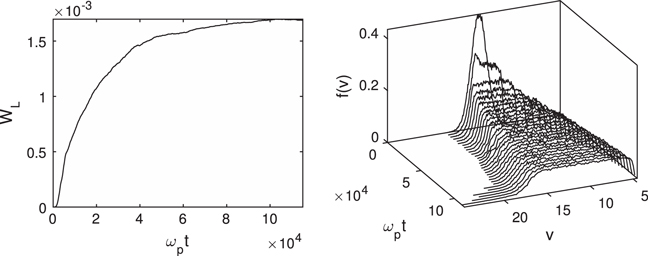
Figure 1. Left: time variation of the normalized spectral energy density WL of the Langmuir waves. Right: time variation of the beam velocity distribution  ; the velocity v is normalized by vT. The main parameters are the following:
 ,
,  ,
, 

Download figure:
Standard image High-resolution imageUp to the time  most features of the system's evolution are in agreement with the predictions of the quasilinear theory of Langmuir waves. However, for
  , short-wavelength density oscillations, which have been identified as IS waves, appear and grow with time along the full length L of the system, as shown by Figure 2 which presents the Langmuir wave energy density
  and the density fluctuations
  as a function of the space coordinate
  at three different times
  28000, and 35000. The short-wavelength density perturbations
  (see Equation (12)) present rather large amplitudes whereas the Langmuir wave packets reveal energy densities
  peaking up to around 0.01. To study these fluctuations in more detail and separate them from the background long-wavelength fluctuations
  , we filter
  and the normalized plasma velocity u, which consists of removing all the Fourier harmonics
  and uk with
  –
– (
( ); we obtain the short-wavelength density and plasma velocity in the form

Note that it is not essential to determine the exact value of  and that we remove the parasitic oscillations that remain after this operation at the edges of the chosen space portion where the filtering is applied. Despite its arbitrariness, this procedure constitutes an effective method for analyzing the properties of the excited IS oscillations.

Figure 2. Left panels: profiles of the normalized wave energy density  (turbulence parameter) at times
  28000, and 35000. Right panels: corresponding profiles of the density fluctuations
  ; short-scale oscillations are growing with time. The space coordinate
  ranges from 0 to the size L of the simulation box. Parameters are the same as in Figure 1.
Download figure:
Standard image High-resolution imageUsing Equation (12), we present in Figure 3 the time and space variations of the turbulence parameter  and the short-scale oscillations
  the full time range of the simulation. The dark lines traveling downward (Figure 3, left) correspond to Langmuir waves propagating along the beam direction with the group velocity
  (
( ). At
). At  IS waves appear (Figure 3, right) that propagate in the beam direction with a velocity around the normalized IS velocity
  . Simultaneously (at
  ), Langmuir waves propagating in the direction opposite to the beam with the group velocity
  can be observed. This picture is in full agreement with the development of a nonlinear decay process during which a Langmuir wave
  (
( ) transfers energy to a counterpropagating Langmuir wave
  of frequency
  and wavenumber
  and an IS wave
  (
( ). During this interaction the conditions of parametric resonance
 and
and 
 should be verified. As is well known from the theory developed in homogeneous plasmas (Kadomtsev 1965; Nicholson & Goldman 1978), those are satisfied if
  and
and  , with
  and
and  corresponding wave dispersions are
  and
and  We show below that in the present case these resonance conditions are fulfilled.
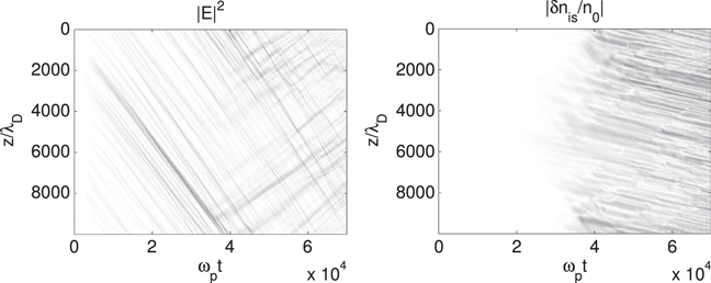
Figure 3. Left: space and time variations of the normalized Langmuir energy density  . Right: space and time variations of the corresponding short-scale density fluctuations
  . Parameters are the same as in Figure 1.
Download figure:
Standard image High-resolution imageLet us study the time evolution of the Langmuir and IS waves' spectra. To distinguish between the IS waves propagating in the positive and the negative directions (i.e., in the direction of the beam propagation and opposite to it, respectively), we calculate the spectra of the Riemann invariants  and
and  where
where  . In the absence of Langmuir waves,
  is conserved along the line
  for IS waves propagating in the positive direction (increasing z in Figure 3) and
  is conserved along the line
  for IS waves propagating in the negative direction (decreasing z in Figure 3). Thus, the spectrum of the energy density of the IS waves can be represented by
  with
with ![${S}_{k}={[{(\rho +u)}^{2}]}_{k}$](https://content.cld.iop.org/journals/0004-637X/809/2/176/revision1/apj517642ieqn127.gif) for
for  and
and ![${S}_{k}={[{(\rho -u)}^{2}]}_{k}$](https://content.cld.iop.org/journals/0004-637X/809/2/176/revision1/apj517642ieqn129.gif) for
for  : Sk is the spectrum of the IS waves with
  propagating in the positive direction and of the IS waves with
  propagating in the negative direction.
The spectra of the Langmuir and the IS waves' energy densities  and Sk are calculated in Figure 4 for the same times as the profiles of
  and
and  in Figure 2. The main peak centered near
  in the
  spectrum corresponds to waves
  excited by the beam instability near the most unstable mode around
  (Figure 4, upper left); note that
  broadens with time toward higher
  (i.e., lower phase velocities
  ); no waves with small
  are visible as wave scattering on the density fluctuations
  is very weak. A second peak (waves
  ) appears at
  near
near  ; it grows with time, eventually reaching the same amplitude as the other one at
  Meanwhile, IS waves
  are excited around
  , as shown by the Sk spectrum at
  (Figure 4, lower left); this peak grows in correspondence with that at
  (note that the peak near k = 0 in the Sk spectrum corresponds to the initial density oscillations and should not be considered here). One can identify the first cascade of the decay process
  . Indeed, the theory of three-waves' resonant decay in a homogeneous plasma predicts that for a parent Langmuir wave at
  we should get
  and
and  , which fits very well with the observations (Figure 4). Further (at
  , not shown here), a second cascade of decay occurs, i.e.,
  providing Langmuir waves with
  and IS waves
  that propagate in the direction opposite to the beam drift, i.e., with a group velocity
  . The secondary decay process is weaker than the first one and the amplitudes of the involved IS waves are smaller. Nevertheless, the cascading process occurs two times, as expected by the theory (no further cascades as
  ); unless damping of waves is included (what is not the case here), there is no threshold for such decay processes.

Figure 4. Upper panels: spectra  of the Langmuir waves (in logarithmic scales) for the same instants of time as in Figure 2, i.e.,
  28000, and 35000, as a function of
  . Lower panels: Corresponding spectra (in logarithmic scales) of the energy density Sk of the IS waves with
  propagating in the positive direction and of the IS waves with
  propagating in the negative direction. Parameters are the same as in Figure 1.
Download figure:
Standard image High-resolution imageThe energy of the IS waves starts to grow when the Langmuir turbulence is almost saturated; thus, one can expect to observe a clear linear stage of the decay instability. Indeed, as shown in Figure 5, the energy  of the short-scale IS oscillations (integrated over the full simulation box) grows exponentially within the time range
  , whereas the corresponding Langmuir energy
  changes only slightly. The growth rate Γ of the IS energy can be estimated as

which is indeed smaller than but close to the maximum growth rate of the decay instability given by Galeev et al. (1975) for monochromatic waves in homogeneous plasmas

Here  is the frequency of the IS waves; then, as
  and
and  (average value) we get
 The uncertainty in the determination of the average value of
  in Equation (14) and the fact that
  is calculated for monochromatic waves in homogeneous plasmas can explain the difference between Γ and the theoretical value
  Note also that, as expected, the nonlinear growth rates Γ and
  are significantly smaller than the typical minimum frequency
  of the waves involved in the decay, ensuring that the collective response of the IS waves can take place as well as the exchanges of energy during the wave–wave coupling.

Figure 5. Time variation of the energy  of the short-scale IS oscillations (thick line and left axis) and of the energy
  of the Langmuir waves (thin line and right axis) integrated over the full system's length
  in logarithmic scales. Parameters are the same as in Figure 1.
Download figure:
Standard image High-resolution imageFinally, we can conclude that our simulations, which were carried out for a small average level Δn ≃ 0.001 of density fluctuations, are consistent with the theory of weak turbulence for Langmuir waves resonantly interacting with IS waves through the channel  . Note that, obviously, the beam instability does not excite a monochromatic wave but a broad wave spectrum. Then, as shown by the above figures, many waves of this wide packet can decay, producing a broad spectrum of daughter waves. The fastest Langmuir decay occurs for waves with the largest field amplitudes, as shown by Equation (14), and the waves with larger k can undergo more decay cascades than those with smaller k. After the occurrence of several cascades, the Langmuir energy can be accumulated within the region
  , where waves cannot continue to decay but where the process of scattering off ions can become effective (see e.g., Cairns 2000; Kontar & Pecseli 2002). However, this problem is not considered here.
The influence of the background density inhomogeneities on the system's dynamics becomes significant only when Δn approaches or exceeds the threshold  , as shown by our previous works (Krafft et al. 2013; Volokitin et al. 2013) and the study we present herein concerning wave decay. We will consider in details successively two cases, when Δn = 0.01 and Δn = 0.02.
3.2. Langmuir Wave Decay in Inhomogeneous Plasmas with Random Density Fluctuations
When the average level of density fluctuations Δn becomes of the order or larger than the threshold  , the dynamics of the system is strongly influenced by the scattering of the waves on the density inhomogeneities. Indeed, the wave–particle resonance conditions are violated due to the random variations of the waves' phase velocities
  ; as a consequence, and compared to the homogeneous plasma case, the rate of growth of the Langmuir wave energy emitted during the bump-on-tail instability is decreased, while the relaxation time of the beam is increased. Moreover, due to their interactions with the density inhomogeneities, Langmuir waves with larger k can transfer part of their energy to Langmuir waves with smaller k, which in turn can damp and accelerate beam electrons of velocities
  up to
up to  and more. Note also that in plasmas with
  Langmuir waveforms tend to form spatially localized and clumpy wave packets.
The presence of fluctuating density gradients generating various processes of wave reflection, refraction, and scattering as well as wave energy focusing alter the development of parametric instabilities occurring in plasmas with long-wavelength density inhomogeneities; some of the first reasons are, for example, the random variations of the wave frequencies and thus of the resonance conditions between waves,  , and the modification of the distribution of Langmuir wave energy in the k-space. Thus, the influence of
  on the nonlinear dynamics of waves during Langmuir turbulence is important, as revealed by the following simulation results.
Figure 6 shows the time evolution of the Langmuir wave spectral energy WL and of the beam electron velocity distribution  in a plasma with
  near the threshold
  . One observes the presence of accelerated electrons (right panel) and the linked saturation of the wave energy growth (left panel, to compare with Figure 1).
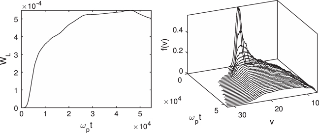
Figure 6. Left: time variation of the normalized spectral energy density WL of the Langmuir waves. Right: time variation of the normalized beam velocity distribution  . The main parameters are the following:
 ,
,  ,
, 

Download figure:
Standard image High-resolution imageProfiles of the Langmuir wave energy  and the density fluctuations
  along the simulation box of length L are presented in Figure 7 for three different times
  36000, and 52000. One can see that Langmuir wave packets are focused and localized within a wide space region where the density fluctuations are forming a well (upper panels). Note that such observations were also done for density perturbations forming humps and not only depletions, as in the case presented here. After some time (middle panels) the local structure of the Langmuir waves, which form a set of more or less separated packets, is conserved despite the modification of the density profile. However, after the appearance of IS waves of noticeable intensity, the structure of the Langmuir packets becomes much more irregular and chaotic in the space region where short-scale density oscillations are rising (lower panels). This is due to the decay of Langmuir waves and to the consequent redistribution of energy between them, as shown below.
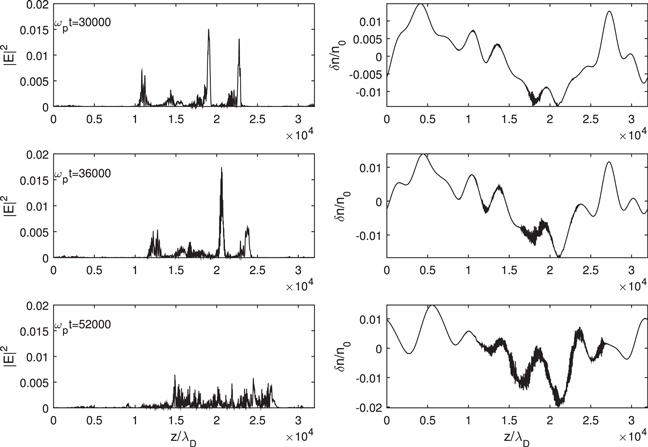
Figure 7. Left panels: profiles of the Langmuir wave energy  (turbulence parameter) at times
  36000, and 52000. Right panels: corresponding profiles of the density fluctuations
  The space coordinate
  ranges from 0 to the size L of the simulation box. The parameters are the same as in Figure 6.
Download figure:
Standard image High-resolution imageThe spectra of the Langmuir and IS waves, shown in Figure 8 for the same times as in Figure 7, present features similar to those observed in Figure 4 for the case of small  ; indeed, one can observe peaks corresponding to the development of a decay instability. However, due to the presence of randomly varying density inhomogeneities, some differences exist between the theory of decay in quasi-homogeneous plasmas and the observations, as will be discussed below.

Figure 8. Upper panels: spectra  of the Langmuir waves, in logarithmic scales, for the same times as in Figure 7. Lower panels: corresponding spectra (in logarithmic scales) of the energy density Sk. The full ranges of space (box of length
  ) and time of the system are considered (global spectra). The parameters are the same as in Figure 6.
Download figure:
Standard image High-resolution imageFirst, the wavenumber of the Langmuir mode observed near  at
at  and 36000 is consistent with the value expected for a first decay cascade, i.e.,
  ; the value of kL is determined by the location of the highest peak with
  in the Langmuir spectrum at
  (upper left panel, Figure 8), i.e.,
  (here
(here  and
and  ; note that the most excited Langmuir waves have phase velocities
  so that
  ). At the same time, the largest peak in the IS spectrum is centered near
  , which is very close to the expected wavenumber
  of IS waves produced during a first decay cascade. Moreover, the peak at
  in the Langmuir spectrum (upper left and middle panels) represents the mode
  generated during a second decay cascade, for which the corresponding IS wavenumber is expected at
  , which is close to the mode at
  visible in the IS spectrum (lower middle panel). Let us stress that the complex peak structure in the low-frequency spectra can be attributed to the fact that several decay instability regions exist and interfere one with another. Moreover, effects due to Langmuir waves' reflections on the density humps are essential and lead to the widening of the peaks in the corresponding wave spectra.
Second, one important difference compared to the quasi-homogeneous plasma case is that wave decay occurs in localized space-time regions. Indeed, for a given moment in the time range when decay occurs, there are not many occurrences of decay spread accross the full range of z (as in Figure 3), but the development of such a process can be observed only in two or three localized space regions. In this case, the processes of scattering, reflection, and/or 1D refraction modify the waves' propagation locally, depending, for example, on the presence along the waves' paths of more or less sharp gradients, deep wells, or wide humps, so that these waves can lose some part of their energy during their propagation, reducing by this fact the possibility of being submitted to further decay processes along z. To understand how a locally arising nonlinear interaction of Langmuir waves with density fluctuations develops, let us focus our attention on finite portions ![$[{z}_{1},{z}_{2}]$](https://content.cld.iop.org/journals/0004-637X/809/2/176/revision1/apj517642ieqn229.gif) of the simulation box. Figure 9 shows the spatio-temporal evolution of the Langmuir wave energy
of the simulation box. Figure 9 shows the spatio-temporal evolution of the Langmuir wave energy  and the short-scale IS density fluctuations
  in the subbox
 ![$[{z}_{1},{z}_{2}]=[13000,24000]{\lambda }_{{\rm{D}}}$](https://content.cld.iop.org/journals/0004-637X/809/2/176/revision1/apj517642ieqn232.gif) , during the time interval
, during the time interval  . One can see the formation of three main regions of IS wave activity (right panel), which broaden and eventually intersect. Note the emergence of IS waves traveling in the direction opposite to the beam propagation with a group velocity around
  , starting, for example, at
  and
and  : they correspond to the development of a second cascade of decay instability (see also above).
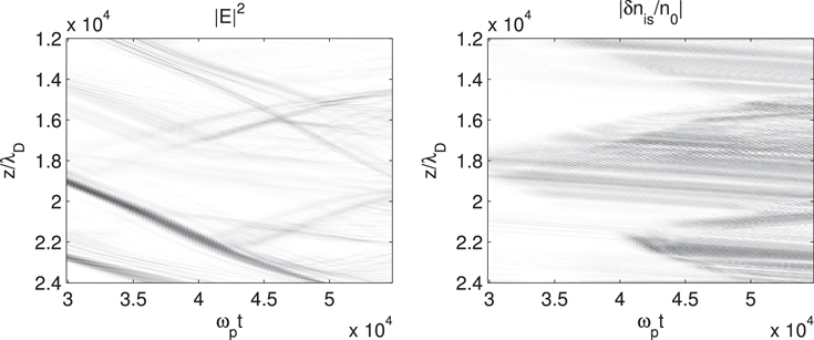
Figure 9. Space and time variations of  (left) and of the corresponding short-scale density fluctuations
  (12) (right), in the limited area
 ![$[13000,24000]{\lambda }_{{\rm{D}}}$](https://content.cld.iop.org/journals/0004-637X/809/2/176/revision1/apj517642ieqn239.gif) and during the time interval
and during the time interval  . The parameters are the same as in Figure 6.
Download figure:
Standard image High-resolution imageThe left panel shows that the interactions of Langmuir packets with density fluctuations occur during limited and rather short time durations. Then, as their group velocity  significantly exceeds the IS velocity
  , the Langmuir waves can propagate away from these interaction regions; further, part of their energy can be transferred to Langmuir packets arising from a first decay cascade and propagating in the opposite direction, with a group velocity
  (see, for example, the waves crossing near
  and
and  in the left panel). The beatings between Langmuir waves propagating in opposite directions lead to the generation of IS waves. Processes involving such beatings form a part of the cascade of energy transfer in the weak turbulence theory; however, some differences exist compared to the homogeneous plasma case: due to the presence of background density fluctuations, the decay processes are occurring locally, i.e., only in specific time and space regions.
Figure 10 shows the "local" wave spectra corresponding to Figure 9, i.e., computed within a specific subbox [13000, 24000] during a limited time
  . Those reveal more clearly than the global ones—corresponding to the full space-time domain (Figure 8)—the development of a cascade of energy transfer during the interaction of Langmuir and IS waves. This is particularly visible in the low-frequency spectra, with peaks appearing clearly in the vicinity of
 . In the high-frequency spectra, peaks are excited near
  0.025, 0.065 and 0.09 (upper left panel); the largest one, which corresponds to beam-driven waves, is located at
  As discussed above, a first decay cascade of the Langmuir wave
  starts, giving rise to a counterpropagating Langmuir wave at
 and to an IS wave with
  Further (at
  ), a second decay cascade occurs, providing the peak at
  (upper right panel) and an IS wave
  , propagating opposite to the beam. We obviously recover the same results as above, but with significantly less ambiguity in the interpretation of the spectral peaks.

Figure 10. Upper panels: "local" spectra  of the Langmuir waves, in logarithmic scales, for the same times as in Figures 7 and 8. Lower panels: corresponding "local" spectra (in logarithmic scales) of the energy density Sk. All spectra are computed in the limited space-time area corresponding to
 ![$[13000,24000]{\lambda }_{{\rm{D}}}$](https://content.cld.iop.org/journals/0004-637X/809/2/176/revision1/apj517642ieqn260.gif) and
and  . The parameters are the same as in Figure 6.
Download figure:
Standard image High-resolution imageFigure 11 shows the profiles of the Langmuir wave energy  and the density fluctuations
  within the same spatio-temporal area as in Figures 9–10. IS waves' short-scale oscillations appear first at
  within the region
  ; further they extend over wider space domains, eventually occupying for
  the subarea
 ![$[13000,24000]{\lambda }_{{\rm{D}}}$](https://content.cld.iop.org/journals/0004-637X/809/2/176/revision1/apj517642ieqn267.gif) . However, they do not extend over the whole space profile (see also Figure 7). One can observe that the various space regions of IS waves' generation are separated one from the other. Moreover, in each area where these waves appear, the growth of their energy stops when the Langmuir packets have traveled away and left the interaction region due to the large difference between the IS and the Langmuir waves' group velocities,
. However, they do not extend over the whole space profile (see also Figure 7). One can observe that the various space regions of IS waves' generation are separated one from the other. Moreover, in each area where these waves appear, the growth of their energy stops when the Langmuir packets have traveled away and left the interaction region due to the large difference between the IS and the Langmuir waves' group velocities,  (compare, for example, the panels at
  and
and  ). The escaping Langmuir waves can then interact with IS waves in other space-time regions where such oscillations appear.
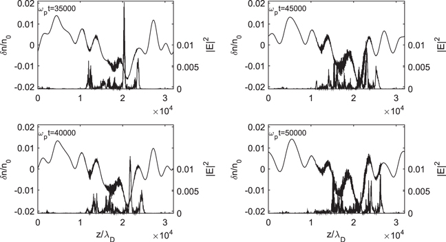
Figure 11. Profiles of the normalized Langmuir wave energy density  (right axis and lower curves in each panel) superposed to the density fluctuations
  (left axis and upper curves), in the area
 ![$[13000{\lambda }_{{\rm{D}}},24000{\lambda }_{{\rm{D}}}]$](https://content.cld.iop.org/journals/0004-637X/809/2/176/revision1/apj517642ieqn273.gif) , at times
, at times 
 , and 50000. Note that the origin of both vertical axes are not coinciding. The parameters are the same as in Figure 6.
Download figure:
Standard image High-resolution imageFigure 12 shows the time variation of the IS and Langmuir waves' energies,  and
and  , respectively, obtained by simulations involving a plasma with density fluctuations of larger average level, i.e.,
  (other parameters being the same as in Figure 1) and computed in the limited domain
 ![${L}_{s}=[13000{\lambda }_{{\rm{D}}},24000{\lambda }_{{\rm{D}}}]$](https://content.cld.iop.org/journals/0004-637X/809/2/176/revision1/apj517642ieqn279.gif) . One can see that, while the plasma waves' energy varies only slightly, the energy of the IS short-scale oscillations
. One can see that, while the plasma waves' energy varies only slightly, the energy of the IS short-scale oscillations  exhibits two periods of exponential growth; each of them corresponds to the growth of a localized IS wave packet rising in a specific region of the subbox Ls. The first period, between
  and
and  corresponds to the crossing of two Langmuir packets of positive but different group velocities; indeed, when a Langmuir packet passes through a density hump, its group velocity can be significantly reduced due to 1D refraction effects. The second period, i.e.,
  (see also Figure 9), corresponds to the occurrence of a first cascade of Langmuir waves' decay, whose growth rate can be estimated as
 (with
(with 
 ; see Equations (13)–(14)).
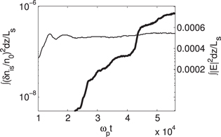
Figure 12. Time variations of the energy densities of the IS short-scale oscillations (bold line, left axis) and of the Langmuir waves (thin line, right axis), i.e.,  and
and  , respectively, in logarithmic scales; the energies are computed within a localized area Ls of the simulation box, in the range
  . The main parameters are the following:
 ,
,  ,
, 

Download figure:
Standard image High-resolution imageLet us present in this case a typical example of Langmuir decay involving several cascades. Figure 13 shows the spatio-temporal variation of the Langmuir wave energy density  and of the short-scale density oscillations
  , in the subbox
 ![$[5000,8000]{\lambda }_{{\rm{D}}}$](https://content.cld.iop.org/journals/0004-637X/809/2/176/revision1/apj517642ieqn298.gif) and the time interval
and the time interval  when the beam instability is saturated. In the left panel, beam-driven Langmuir waves are propagating with
  through the region
 ![$[5000,6700]{\lambda }_{{\rm{D}}}$](https://content.cld.iop.org/journals/0004-637X/809/2/176/revision1/apj517642ieqn301.gif) for
for  ; near
  and
and  their amplitudes are strongly enhanced when they cross another Langmuir packet traveling with
  . At the same time, IS waves propagating with the group velocity
  are excited (right panel).

Figure 13. Space and time variations of  (left) and of the corresponding short-scale density fluctuations
  (right), in the area
 ![$[5000,8000]{\lambda }_{{\rm{D}}}$](https://content.cld.iop.org/journals/0004-637X/809/2/176/revision1/apj517642ieqn309.gif) . The parameters are the same as in Figure 12.
. The parameters are the same as in Figure 12.
Download figure:
Standard image High-resolution imageIn Figure 14, which shows the corresponding profiles of  and
and  (including
  ) at six moments of time, one can see that
  reaches its maximum when the waves approach the local density hump near
  (left middle panel at
  ); at this point, both packets propagating in opposite directions interact and, as a result, some large part of the Langmuir energy is reflected and propagates away with
  (see Figure 13, left, and Figure 14, top right). A similar event can be observed later, near
  and
and  (Figure 13, left): the Langmuir wave decays. Figure 14 at
  and 63000 shows how the counterpropagating packet separates itself from the packet with
  , eventually taking with it almost all the Langmuir energy. The two peaks at
  (Figure 14 , bottom right) can be clearly identified in Figure 13 as the two packets propagating with
  , in the time range
  . Moreover, near
  and
and  , a second decay cascade occurs, giving rise to Langmuir packets propagating with
  and IS waves' oscillations propagating with
  (Figure 13).
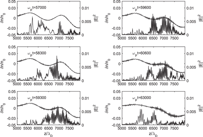
Figure 14. Profiles of the Langmuir wave energy density  (right axis and lower curves in each panel) superposed to the density fluctuations
  (left axis and upper curves), in the area
 ![$[13000{\lambda }_{{\rm{D}}},24000{\lambda }_{{\rm{D}}}]$](https://content.cld.iop.org/journals/0004-637X/809/2/176/revision1/apj517642ieqn331.gif) , at times
, at times 


 60600, and 63000. Note that the zero of both vertical axes are not coinciding. The parameters are the same as in Figure 12.
Download figure:
Standard image High-resolution imageIt is well known from theory (Musher et al. 1995) that decay processes involve several cascades of energy transfer to waves with longer wavelengths. The successive occurrence of two decay cascades was discussed and presented above for the cases of very small or finite average levels of external density fluctuations, i.e., for Δn ≃ 0.001 and Δn ≃ 0.01 (see, e.g., Figure 10). However, one must stress that decay cascading in a plasma with background density fluctuations of finite Δn presents specific features, which we examine now in more detail on the basis of simulation results presented in Figures 12–14. Note first that according to the decay resonance conditions, only three cascades are expected to occur for the beam and plasma parameters considered here. During these successive processes, Langmuir wavenumbers decrease more and more, starting from the value  corresponding to the most excited beam-driven Langmuir waves (not shown here); then, as a consequence of the resonance conditions, the Langmuir wave products of the first, second, and third decay cascades are characterized by the following wavenumbers:
 , and
, and  , whereas for the IS daughter waves we have
 , and
, and  , respectively. A fourth cascade is not possible as the resonance conditions are not fulfilled. An essential point lies in the fact that the Langmuir waves
  coming from the second cascade propagate in the direction of the beam drift and have larger phase velocities than those excited first by the beam instability. So the second decay cascade can play an important role in the acceleration of beam electrons above the initial beam velocity vb.
The first two decay cascades are very clearly observed in Figures 13–14. For  and
and  , two wave packets propagate along the beam direction (
 ) and a third one in the opposite direction (
 ) (Figure 13, left). In the vicinity of
  the packet with
  and with the largest amplitude collides near
  with the packet propagating with
  (see also Figure 14 at
  ). IS waves are generated as a result of the beating between these two colliding packets (Figure 13, right); during this process, the weaker amplitude packet with
  gets energy from the more intense one with
  . This mechanism could be considered as the first cascade of wave energy transformation, but the actual situation is more complicated. Indeed, almost simultaneously, the colliding packet with
  reflects on the density hump presenting a maximum at
  (Figure 14 at
  ). The propagating second packet with
  consequently collides with the amplified packet with
  and with the reflected one (Figure 13, left; Figure 14 at
  ). Their beatings also generate IS waves. At
  two wave packets are traveling in the direction opposite to the beam propagation (Figure 14 at
  ). Later, near
  and
and  a process starts which can be called the second decay cascade, involving one of these packets and generating IS waves propagating in the negative direction (at group velocity
  ) with no signatures of any Langmuir wave reflection (Figure 13, left). At last, near (
 ,
,  ) and (
 ,
,  ), structures similar to a third decay can be observed on the space-time evolution pattern (Figure 13, left); one can indeed observe a small but noticeable enhancement of the IS wave emission along the direction of the beam propagation, near
  and
and  (Figure 13, right), which is expected from a third cascade; however, as the wave packets have amplitudes that are too weak, we are not able to state that this process is actually and certainly a third cascade. Indeed, Figure 15 presents the corresponding local spectra of Langmuir and IS waves at the three time moments
  68000, and 74000; they show that if peaks at
  (upper right panel) and
  (lower right panel) are visible, they are either too weak (IS spectrum) or mixed with other effects (Langmuir spectrum). However, at
  and
and  , the position of some peaks in the IS and Langmuir spectra are very close to those predicted by the resonant wave decay theory in homogeneous plasmas for the first and the second cascades (see the discussion in the previous paragraph). As mentioned above, the spectrum of Langmuir waves for
  does not show clearly distinguishable peaks, which can be explained by two effects, i.e., the propagation of the waves in the inhomogeneous plasma and their exchanges of energy with the beam. At the same time, three main peaks can be observed in the IS spectrum: two correspond to the wavenumbers of the IS wave products of the two first decay cascades, i.e.,
  and
and  , whereas the third one near
  is likely due to a nonresonant wave–wave interaction.

Figure 15. Local spectra (computed in the area ![$[4500,8500]{\lambda }_{{\rm{D}}}$](https://content.cld.iop.org/journals/0004-637X/809/2/176/revision1/apj517642ieqn381.gif) ) of Langmuir and ion sound waves for three moments of time
) of Langmuir and ion sound waves for three moments of time 
 and 74000. The parameters are the same as in Figure 14.
Download figure:
Standard image High-resolution imageFinally, it is important to stress at this stage that it is generally very difficult, if not impossible, to separate the processes of wave reflection on density fluctuations from that of parametric wave–wave interactions; both effects are usually working together in a inhomogeneous plasma, and the origin of the counterpropagating (i.e., with  ) Langmuir waves produced cannot be determined conclusively in most cases. Note also that reflections of Langmuir waves on long-wavelength density inhomogeneities can, in some conditions, favor the emergence of nonlinear decay processes, owing to the appearance of parametric interaction processes involving waves traveling in the direction opposite to the beam propagation. One must also take into account the significant role of the variations of the long-wavelength density fluctuations due to their own dynamics; for example, the local positive gradient of the density hump in Figure 14 disappears for
  and conditions for IS wave generation in the vicinity of this region become less favorable than when Langmuir energy can focus on the gradients of the humps near some reflection points.
4. DISCUSSION AND CONCLUSION
Simulations have shown that three-wave decay processes including several cascades can occur in inhomogeneous plasmas as those of the solar wind in the source regions of type III bursts and, in particular, in the course of Langmuir turbulence in the presence of electron beams. Wave–wave interaction processes where a Langmuir wave decays into a Langmuir and where IS waves can be observed in plasmas with average levels of density fluctuations up to a few percent. Decay has been notably identified by the simultaneous presence of peaks in the high- and low-frequency wave energy spectra, at the wavenumbers of the mother and the daughter waves, in agreement with the waves' resonance conditions. Moreover, the growth rate of the IS energy has been shown to fit with the predictions of the parametric decay theory for homogeneous plasmas and monochromatic waves, at least up to Δn ≃ 0.02. A very good agreement between the wavenumbers predicted by this theory and our simulations of Langmuir turbulence in inhomogeneous plasmas has been observed. This is due to the fact that the waves' dispersion equations are not significantly modified by the irregularities and that the wavenumbers' shifts due to the density fluctuations are smaller than the spectral widths of the peaks.
For small values of Δn below the threshold, i.e.,  , three-wave decay processes occur commonly during Langmuir turbulence and can arise after some time in all space regions; moreover, they can be described with a rather good agreement by the weak turbulence theory for monochromatic waves in homogeneous plasmas. In this case, Langmuir turbulence does not present focused peaks along the space profiles (with a lack of Langmuir energy in some regions), but the wave energy is distributed roughly uniformly along the simulation box: wave decay is not a localized process and can evolve in time until its own saturation. On the contrary, when
  , several other effects such as wave scattering, reflection, or 1D refraction, for example, can compete with the decay processes whose duration is more limited and which take place locally in space-time locations where the physical conditions allow their appearance. These specific regions can be of various nature and are not only concerning the vicinity of reflection points on the density fluctuations' gradients where the Langmuir energy can be accumulated and focused before the decays start. In this case, as the Langmuir group velocity vg is generally much larger than the IS group velocity cs, the decay processes are not stopped due to nonlinear wave saturation but to kinematic effects, when the fastest Langmuir packets escape the localized regions where they locally interact with IS waves. However, in the asymptotic stage of the system's evolution, short-scale IS oscillations can exist along the whole space profile, due to the fact that vg is significantly larger than cs and that the Langmuir packets have time to travel through the density profile several times during the entire time of the simulation. Moreover, IS oscillations survive for a long time and can interact several times with the same Langmuir packets passing again in their neighborhood or with other arriving ones.
Generally, the larger Δn is (and/or the smaller the wavelengths of the fluctuations), the more decay processes become rare, as they can be overcome by scattering processes of waves on the density inhomogeneities. For large values of Δn lying significantly above the threshold (i.e.,  ), decay cannot be observed or only rarely and under specific local conditions; in this case, the scattering of the waves on the inhomogeneities, which occurs on a much shorter timescale than the decay process, tends to destroy the coherency between the waves necessary for decay. For example, the occurrence of wave decay is observed in our simulations for
  , even if this process is mostly overcome by reflection phenomena; however, for
  , no example of wave decay could be found for the physical parameters used.
While decay processes in quasi-homogeneous plasmas are more likely to occur when the beam is almost fully relaxed, such effects can start in a inhomogeneous plasma well before the beam is relaxed due to reflection processes and to the accumulation of energy near the reflection points on the density profiles. Indeed, the interferences between Langmuir waves can become more frequent because the possibilities of generating counterpropagating Langmuir waves are enhanced due to the presence of density fluctuations. Then, in some cases, reflection processes can favor the appearance of a decay process, i.e., increase its efficiency in its early stage, due to the coupling of Langmuir waves with amplitudes above the thermal level.
Langmuir wave decay allows the transfer of energy to smaller k waves, which can in turn accelerate beam electrons and generate high-energy tails. In particular, if the first decay cascade provides waves propagating in the direction opposite to the beam, the second cascade's Langmuir products propagate along the beam direction and thus can interact with beam particles of velocities larger than the initial beam velocity vb. However, they usually have small k and phase velocities around or exceeding  , so that all of them cannot be in resonance with the accelerated particles, whose largest velocity exceeds the velocity
  only for very long simulations. The next cascade processes can only shift the Langmuir waves to large resonance velocities and cannot affect the acceleration of beam particles. In the cases presented above, we can observe an increase with time of the largest velocity of the population of accelerated particles, beginning from
  when the second decay cascade starts (Figure 16; see also Figure 13). Such a process is, however, occurring in advanced stages of the beam relaxation, and thus is believed to play a minor role compared to the acceleration induced by the presence of randomly fluctuating density inhomogeneities. A more detailed study will be carried out in a forthcoming paper.
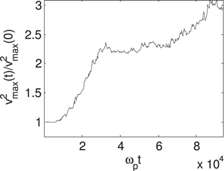
Figure 16. Variation with time of the maximum (normalized) square velocity of the population of accelerated particles; a second increase occurs near  , when the second decay cascade starts. The parameters are the same as in Figure 12.
Download figure:
Standard image High-resolution imageFinally, the occurrence of decay cascades has a noticeable influence on the redistribution of energy between the different k-scales of the Langmuir turbulence, leading to the appearance of specific modulation features in the corresponding Langmuir waveforms. Thus, wave–wave coupling can play a significant role in shaping these waveforms and producing the clumpy and characteristic modulation patterns observed by the satellites STEREO and WIND. Two examples are shown in Figure 17, for the parameters of Figures 12–16, i.e., when Δn ≃ 0.02. Let us simulate what would observe a virtual satellite starting at time  and position
  and moving with a velocity
  ; this satellite concludes its travel at
  , arriving at the position
  ; during its path, it passes through the region where the decay process occurs, i.e., within the space-time domain
  and
and  (see Figure 13). On the other hand, when the satellite starts at the same time but at another location
  , for example, and travels with the same velocity, it does not encounter any wave decay process, as such effect is not observed in the corresponding space-time range. Let us now compare in Figure 17 the waveforms observed by the virtual satellite for these two cases, respectively, i.e., the normalized electric fields
  registered as a function of time (Krafft et al. 2014). One observes in the upper panel (
 ) that specific modulation features revealing wave–wave beating appear within the range
  , when the satellite travels from
  to
to  , which corresponds exactly to the space-time domain where decay occurs (see Figures 13–14).

Figure 17. Langmuir waveforms (registered electric fields ES as a function of time) that would be observed by a satellite moving at a velocity  and starting at positions
  (upper panel) and
  (lower panel) at time
  ; the satellite travels until the time
  . The parameters are the same as in Figure 12.
Download figure:
Standard image High-resolution image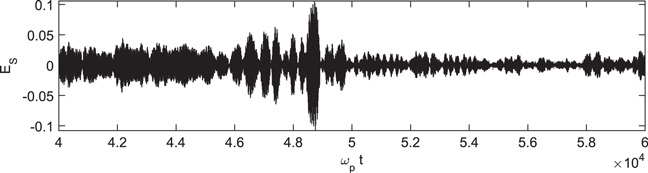
Figure 18. Langmuir waveform (registered electric field ES as a function of time in arbitrary units) that would be observed by a satellite moving at a velocity  and starting at a position
  at time
  ; the satellite travels until the time
  . The parameters are the same as in Figure 12, but with
  .
.
Download figure:
Standard image High-resolution imageOn the contrary, this kind of modulated structures are not visible in the waveform when the satellite starts at  (lower panel), i.e., when it does not cross any decay event. Such a result is in good agreement with the observations by the satellite STEREO reported recently in Graham & Cairns (2013), where their Figure 4 shows Langmuir waveforms observed before and after an electrostatic decay, in conditions very similar to ours (in particular, the electric field has a negligible perpendicular component); before decay, the amplitude of the waves varies smoothly and slowly, whereas after the decay a modulation pattern revealing wave–wave beating can be observed.
Another example is shown in figure 18 for the case of a plasma with a larger average level of inhomogeneities, i.e., Δn ≃ 0.03, where the other parameters are similar to those of Figures 12–16. A satellite passes with the velocity  through the region where the simulations evidenced a Langmuir decay. As a consequence, the waveform exhibits, during the time lapse
  when the decay process occurs, modulation features characteristic of wave beating.
Finally, in order to fit more closely to realistic physical conditions, we have performed simulations including finite ion and electron damping factors calculated taking into account bulk plasmas with nonthermal electron and ion Kappa tails. Figure 19 presents the time variation of the IS energy and the space-time evolution of the Langmuir energy density, respectively. The upper panel shows a significant growth of the IS energy near  whereas, around this time, one can observe in the lower panel the appereance of backscattered Langmuir waves propagating with negative group velocities. Therefore, even for significant (but moderate, due to the typical electron to ion temperature ratios
  ) values of the ion and electron damping factors
  and
and  , damping effects due to the presence of nonthermal electron and ion tails do not suppress the occurence and the fulfillment of the Langmuir wave decay processes. Moreover, those can even be identified more clearly due to the more or less efficient suppression of some wavelengths in the spectra.
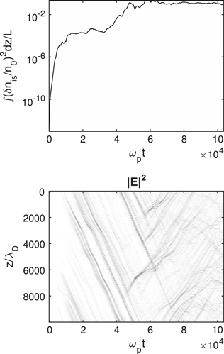
Figure 19. Upper panel: time variation of the energy densities of the IS short-scale oscillations. Lower panel: space and time variations of  , in the case when Landau damping on ions and electrons is taken into account, due to the presence of nonthermal Kappa tails in the bulk plasma velocity distribution. The main parameters are the following:
 ,
,  ,
,  ,
,  .
.
Download figure:
Standard image High-resolution image
This work was granted access to the HPC resources of IDRIS under the allocation 2013- i2013057017 made by GENCI. This work has been done within the LABEX Plas@par project, and received financial state aid managed by the Agence Nationale de la Recherche, as part of the programme "Investissements d'avenir" under the reference ANR-11-IDEX-0004-02. C.K. acknowledges the "Programme National Soleil Terre" (PNST) and the Centre National d'Etudes Spatiales (CNES, France). V.K. acknowledges the financial support from CNES through the grant "STEREO invited scientist."