


ABSTRACT
We present a survey of 429 coronal prominence cavities found between 2010 May and 2015 February using the Solar Dynamics Observatory (SDO)/Atmospheric Imaging Assembly limb synoptic maps. We examined correlations between each cavity's height, width, and length. Our findings showed that around 38% of the cavities were prolate, 27% oblate, and 35% circular in shape. The lengths of the cavities ranged from 0.06 to 2.9  . When a cavity is longer than 1.5
  , it has a narrower height range (0.1–0.3
  ), whereas when the cavity was shorter than 1.5
  , it had a wider height range (0.07–0.5
  ). We find that the overall three-dimensional topology of the long, stable cavities can be characterized as a long tube with an elliptical cross section. We also noted that the circular and oblate cavities are longer in length than the prolate cavities. We also studied the physical mechanisms behind the cavity drift toward the pole and found it to be tied to the meridional flow. Finally, by observing the evolution of the cavity regions using SDO/Helioseismic Magnetic Imager (HMI) surface magnetic field observations, we found that the cavities formed a belt near the polar coronal hole boundary; we call this the cavity belt. Our results showed that the cavity belt migrated toward higher latitude over time and the cavity belt disappeared after the polar magnetic field reversal. This result shows that cavity evolution provides new insight into the solar cycle.
Export citation and abstract BibTeX RIS
1. INTRODUCTION
Coronal prominence cavity evolution provides insight into the cause of the solar cycle. The solar cycle has always been an important topic of research in solar physics. It is a dynamo process involving the transformation of a poloidal magnetic field into a toroidal and from toroidal bands to a poloidal field, with the polarity becoming opposite to what was present earlier (Parker 1955; Dikpati & Charbonneau 1999). The cycling dynamo is characterized by the equatorward migration of sunspots as well as meridional flow. Meridional flow is the latitudinal flow of material from the equator toward the poles at the surface and from the poles to the equator below the surface. An inner return flow has been proposed to carry material from the mid-latitudes to the equator in about 11 years (Hathaway & Rightmire 2010).
The timing of polar field reversal has been studied using the polar magnetic field (Babcock 1959; Scherrer et al. 1977; Sun et al. 2015) and coronal hole boundaries (Waldmeier 1981; Webb et al. 1984; Karna et al. 2014). During polar reversal, there is maximum sunspot activity, the polar coronal holes shrink and almost disappear, and the polar magnetic field decreases through zero and reverses its polarity. Moreover, the migration of prominences toward the pole at the beginning of the solar cycle has been reported (Topka et al. 1982; Makarov & Sivaraman 1989; Mouradian & Soru-Escaut 1994; Shimojo et al. 2006; Li et al. 2008; Shimojo 2013).
In this article, we investigate how the coronal prominence cavity provides new insight into the global magnetic field evolution. Coronal cavities are circular, half-circular, or elliptical dark regions observed above the solar limb in white light and EUV coronal images as shown in Figure 1. In coronagraph observations, a cavity surrounds the prominence in both cases: prior to eruption in the lower corona and as a part of coronal mass ejections (CMEs) in the outer corona (Gibson et al. 2006). Cavities come in a range of sizes and shapes, from small ones associated with active regions to large cavities associated with large-scale, longitudinally extended polar crown filaments (Fuller et al. 2008). More than two-thirds of all CMEs originate from filament eruptions (St. Cyr & Webb 1991; Gopalswamy et al. 2003). Sometimes, even after an eruption, prominence and cavity remnants can remain or even reform at the same location (Gibson & Fan 2006). Cavities represent a much larger volume than that of the prominence, and so are an important part of the prominence cavity magnetic structure (Rachmeler et al. 2013; Gibson 2015).
We present a survey of 429 cavities found in data from the Atmospheric Imaging Assembly (AIA, Lemen et al. 2012) and Helioseismic Magnetic Imager (HMI, Schou et al. 2012) on board the Solar Dynamics Observatory (SDO, Pesnell et al. 2012). We studied the three-dimensional (3D) morphological structure of the cavities that appeared between 2010 May 20 and 2015 February 1, using the Limb Synoptic Maps described in Karna et al. (2015 hereafter Article 1). We measured the length, height, width, and heliographic longitudes and latitudes of the appearance and disappearance of the cavity. We also examined the correlations between the heights, widths, and lengths of the cavities in the catalog. We also found that the cavities formed a belt moving toward the polar region over time; we call this new belt the "cavity belt," an unquestionable piece of evidence for surface meridional flow. The article is organized as follows. In Section 2, we describe data measurements. In Section 3, we present our results. In Section 4, we discuss what we are able to draw from our observations and compare our results with other work. In Section 5, we summarize our results and present our conclusions.
2. MEASUREMENTS
We used limb synoptic maps to identify cavities. Limb synoptic maps are constructed from annuli above the solar limb as described in Article 1. The limb synoptic maps are available at the George Mason University (GMU) Space Weather Lab http://spaceweather.gmu.edu/projects/synop. As described in Article 1, a cavity appears as an elongated dark region in both AIA 193 Å and AIA 211 Å wavelength synoptic maps, and we see a prominence at the same location in AIA 304 synoptic maps. We identified 429 cavities since the launch of SDO. We measured the length of each cavity, one advantage of the measurements from the limb synoptic maps described in Article 1. Height and width are measured using the snapshot images at the middle time frame of the cavity's evolution.
We have made the following assumptions when counting the cavities.
- 1.If cavities appear at almost the same locations during a Carrington Rotation and also during the following Carrington Rotation, then they are counted as two different cavities.
- 2.If a cavity disappears for more than 48 hr (all 48 hr in the sequence of snapshot images) and reappears at the same latitude, then it is counted as a new cavity.
3. RESULT
We observed 429 cavities in four and a half years of data. The online cavity catalog lists the number of cavities seen in each Carrington Rotation from CR 2097 to CR 2159 (2010 May 20–2015 February 1), along with the length, height, width, and heliographic longitudes and latitudes of the appearance and disappearance of the cavity.

Figure 1. Snapshot images of cavity C21295746S as seen on the eastern limb on 2012 October 30 in the SDO/AIA 193 Å passband.
Download figure:
Standard image High-resolution imageFigure 2 shows how the height of each cavity varies with the width of the cavity. The heights of the cavities range from 0.08  to 0.5
  , whereas the widths vary from 0.09
  to 0.4
  . We arbitrarily defined the circular boundary
  to be in the range 0.9–1.1. In the plot, the blue line with error bars represents the region of circular cavities. Cavities falling above the blue line are prolate in shape and cavities falling below the blue line are oblate in shape. The plot shows that around 38% of cavities are prolate, 27% of cavities are oblate, and 35% of cavities are circular in shape. The typical error of measurement is 3 pixels (less than 1%), which is based on the standard deviation of measurement data to the ellipse fitting of the cavity. There is a weak linear correlation between height and width. The correlation coefficient between height and width is approximately r = 0.6.
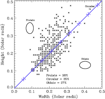
Figure 2. Height vs. width. Blue line with an error bar (10%) represents the region of circular cavities. Cavities falling above the blue line are prolate in shape and cavities falling below the blue line are oblate in shape.
Download figure:
Standard image High-resolution imageFigure 3 shows how the length of each cavity varies with the height of the cavity. The lengths of the cavities range from 0.06  to 2.9
  . One quarter of the cavities are longer than a solar radius. Cavities with length greater than 1.5
  have a narrower height range (0.1–0.3
  ), whereas cavity lengths smaller than 1.5
  have a wider height range (0.07–0.5
  ). The two red lines are estimated boundary lines that show how, with increasing cavity length, the height range decreases. This result implies that high-lying long cavities are unstable and subject to eruption. We find that the overall 3D topology of long, stable cavities is a long tube with an elliptical cross section. We also notice that the circular and oblate cavities are more common in long cavities and infer that they are more stable than prolate cavities. Figure 3 also shows that the prolate cavities on average have a higher height compared to the other shapes. The shorter length and higher height of the prolate cavities imply that prolate cavities are more likely to erupt. Forland et al. (2013) conducted a survey of cavities using 19 months of SDO/AIA data. They noted specific characteristics of the cavities in relation to their eruption as CMEs and concluded that, on average, eruptive cavities are narrow, high-centered, and with a base noticeably above the limb.
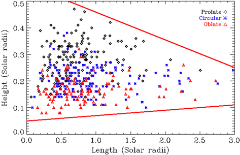
Figure 3. Height vs. length. The black diamonds, blue asterisks, and red triangles represent the prolate, circular, and oblate shapes of the cavities. The two red lines are the boundary of a region that shows how the height range narrows with increasing cavity length.
Download figure:
Standard image High-resolution imageWe plot each cavity's average latitude with time over the SDO/HMI magnetic butterfly diagram as seen in Figure 4. A magnetic butterfly diagram is produced by averaging the radial magnetic fields from HMI synoptic maps (Liu et al. 2012) over longitude for each solar rotation described by Karna et al. (2014).
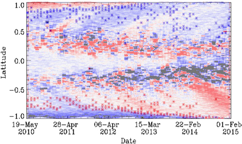
Figure 4. Time-latitude Butterfly diagram. The blue and red asterisks are cavity average latitude positions obtained from the limb synoptic map appearing in the northern and southern hemispheres. Red regions have negative polarity, and blue regions have positive polarity.
Download figure:
Standard image High-resolution imageIn Figure 4, we note that the cavities form a belt moving toward the polar regions in both hemispheres; we call this the "cavity belt." The evolution of cavity locations apparently depends on the sunspot cycle. Sunspots start each new cycle by emerging at relatively high latitudes and emerge at progressively lower latitudes as the cycle progresses. In a time-latitude butterfly diagram, we can see the active region field exhibiting a strong equatorward motion. Meanwhile, cavities progress toward the pole until the polar magnetic field reverses (as seen in the butterfly diagram when the magnetic field changes sign) and then appear at more random locations as seen in the northern hemisphere. Meanwhile, in the southern hemisphere, the cavity belt is still seen in the polar latitudes (see Figure 4). The appearance of cavities at random locations has not been observed in this hemisphere, as our data stops soon after the southern pole reversal. From the HMI data (Figure 4), we note that the northern pole reversed in late 2012, while the southern polar magnetic field reversed in late 2014.
4. DISCUSSIONS
As shown earlier, the cavity drift toward the pole is apparently related to the polar reversal. By observing the cavity through surface magnetic field observations from HMI, we showed that the cavity belt was formed near the polar coronal hole boundary. The cavity belt disappeared after the polar magnetic field reversal. The HMI magnetic butterfly diagram showed that the northern pole reversed in late 2012, however, the cavity belt disappeared several Carrington Rotations later. On the other hand, the southern pole reversed polarity in late 2014 (see Figure 4). We compared our magnetic butterfly diagram with Hathaway's magnetic butterfly diagram (Figure 17 of Hathaway 2015), and in both we noticed that the southern magnetic field reversed in late 2014. However, the results from the solar polar fields strengths measured by the Wilcox Solar Observatory (WSO), show that the northern polar field changed its polarity first in 2012 June but fluctuated around zero magnitude from 2014 March until late in 2014, while the southern polar field reversed in 2013 July (see Figure 5).
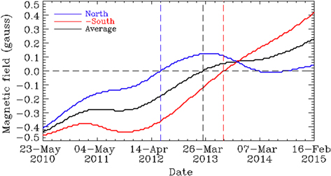
Figure 5. Solar polar magnetic strength data from WSO, filtered by a 20 nHz lowpass filter. The blue, red, and black lines represent the magnetic field strength at the north pole, south pole, and their average. Vertical lines represent the estimated time of the magnetic field reversals.
Download figure:
Standard image High-resolution imageOur HMI results for the timing of the polar field reversal in the northern hemisphere (Figure 4) differ by six months from the filtered WSO data. HMI data shows that the southern polar magnetic field reversed in late 2014, which is 1.5 years after the WSO reversal in mid-2013. Moreover, the cavity belt disappeared from the northern hemisphere within a few rotations, and the cavity belt disappeared in the southern pole just around the time of HMI reversal. Our cavity belt disappearance timing agrees better with the reversal timing from the HMI data.
The monthly sunspot Number (Figure 6) peaked in late 2011, primarily due to activity in northern hemisphere, whereas activity in the southern hemisphere peaked in 2014 February. Comparing Figures 4 and 6 shows that the northern pole reversed one year after sunspot maximum while the southern sunspot number peaked nine months earlier than southern pole reversal.
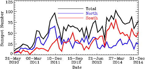
Figure 6. Monthly sunspot average. Blue and red represent the northern and southern hemispheric sunspot numbers, respectively. The black line represents the total sunspot number.
Download figure:
Standard image High-resolution imageOne key question is what causes the cavity belt? To answer this, we applied a linear fit to the variation of cavity latitudes within the belts and calculated the cavity belt migration speed from the slope of the fit. The cavity belt migration speeds in the northern and southern hemisphere were 5.0 m s−1 and 3.7 m s−1, respectively. We note two points from our result. First, our result is consistent with the meridional flow speed of  m s−1 at 75° latitude from Hathaway & Rightmire (2010) based on the magnetic features from 1996 May to 2009 June observed by the Michelson Doppler Imager on board the Solar and Heliospheric Observatory. Our results suggest that the cavity drift toward the pole forming the cavity belt is due to the meridional flow. Second, cavity belt drift is slower in the southern hemisphere. The late reversal in the southern pole may be due to slower meridional flow in the southern hemisphere. Moreover, we also noticed that from time to time cavities appear to follow surges in both hemispheres.
The migration of the prominences toward the poles during the ascending phase of the solar cycle has been reported by several authors (Topka et al. 1982; Makarov & Sivaraman 1989; Mouradian & Soru-Escaut 1994; Shimojo et al. 2006; Li et al. 2008; Shimojo 2013). For example, Shimojo et al. (2006) compared prominence activity data from 1992 July to 2004 December from the Nobeyama Radioheliograph (NoRH) with butterfly diagrams obtained from synoptic Carrington maps of Kitt Peak National Observatory magnetograms. They concluded that the drift of the prominences follows the poleward motion of the magnetic flux until the reversal of the polar polarity; after reversal, filaments slowly migrate toward the equator. A similar result was obtained by Li et al. (2008) from the latitudinal migration of filament activity over the full solar disk using the Carte Synoptique solar filament archive. Our results also show that the cavity belts move toward higher latitudes before the pole reversal. From Figure 4, we can see that soon after reversal in the northern hemisphere the cavity belt disappeared, and that later cavities appeared at random latitudes.
Topka et al. (1982) used Hα synoptic charts from 1964 to 1980 and calculated a poleward drift velocity of about 10 m s−1, which is twice our meridional flow speed in the northern hemisphere. This difference may come from looking at two different solar cycles. Shimojo (2013) extended the NoRH prominence data until 2013 March, calculated the migration velocities in the northern hemisphere to be 5.2 m s−1 for Solar Cycle 24, and concluded that a poleward motion of the prominences was an indicator of the meridional flow. In the southern hemisphere, only two prominence activities occurred at over −65° latitude after 2009, and therefore poleward expansion was not measured. Our cavity belt drift speed from the northern hemisphere agrees with that from Shimojo (2013).
Moreover, we examined whether there was a trend toward having a larger fraction of oblate cavities as the solar cycle progressed, but we found no significant correlation of shape with solar cycle phase.
5. SUMMARY AND CONCLUSION
We present a survey of 429 coronal prominence cavities found between 2010 May and 2015 February using SDO/AIA limb synoptic maps. Our findings showed the following.
- 1.38% of cavities are prolate, 27% oblate, and 35% circular in shape.
- 2.Cavities longer than 1.5
 have a narrower height range (0.1–0.3 ), whereas cavities shorter than 1.5 have a wider height range (0.07–0.5 ).
 - 3.The overall 3D topology of the long, stable cavities can be characterized as a long tube with an elliptical cross section.
- 4.Circular and oblate cavities have longer lengths than prolate cavities.
- 5.Early in a sunspot cycle, cavities form a belt moving toward the polar region with time; we call this the cavity belt.
- 6.The cavity belt migrated toward higher latitude with time and the cavity belt disappeared after the polar magnetic field reversal.
- 7.The HMI magnetic butterfly diagram showed that the northern pole reversed in late 2012, however, the northern cavity belt disappeared several Carrington Rotations later. Meanwhile, the southern pole reversed polarity in late 2014 and the cavity belt disappeared exactly at the time of southern pole reversal.
- 8.The HMI magnetic field diagram northern polar field reversal timing (late 2012) differs by six months from the filtered WSO data (mid 2012), and the HMI results (late 2014) from the southern hemisphere are one and a half year delayed in comparison to WSO data (mid-2013). In the WSO data, the northern hemisphere returned to near zero in 2014 and only recently appears to have reversed.
- 9.Cavity belt migration speeds in the northern and southern hemisphere were 5.0 and 3.7 m s−1, implying cavity belt migration is due to meridional flow.
- 10.The late reversal in the southern pole may be due to slower meridional flow in the southern hemisphere.


Our analysis shows that the cavity belt migrates toward higher latitudes at the time of magnetic field reversal and could be used to establish the time of polar magnetic field reversal. Our result gave us new insight to look at the global magnetic field. This study shows that the cavity evolution provides another dimension of information on the solar cycle.
N.K. thanks the Schlumberger Foundation Faculty for the Future for supporting this research. W.D.P. was supported by NASA's Solar Dynamics Observatory. J.Z. is supported by NSF AGS-1156120 and NSF AGS-1249270. The authors thank Sarah Gibson for many useful suggestions. The AIA and HMI data are courtesy of NASA/SDO and the AIA and HMI Science Investigation Teams. The GMU AIA Synoptic Maps Dataset can be accessed at http://spaceweather.gmu.edu/projects/synop. The monthly international sunspot numbers, separated by hemisphere, were obtained from http://www.ngdc.noaa.gov/stp/space-weather/solar-data/solar-indices/sunspot-numbers/hemispheric/lists/. Solar Polar Field Strength data, separated by hemisphere were obtained from http://wso.stanford.edu. The HMI synoptic maps were obtained from http://jsoc.stanford.edu/data/hmi/synoptic/. We would like to thank the anonymous referee for useful suggestions that helped improve the paper.