


ABSTRACT
We present H-band observations of β Pic with the Gemini Planet Imager's (GPI's) polarimetry mode that reveal the debris disk between ∼0 3 (6 AU) and ∼17 (33 AU), while simultaneously detecting β Pic b. The polarized disk image was fit with a dust density model combined with a Henyey–Greenstein scattering phase function. The best-fit model indicates a disk inclined to the line of sight (
 ) with a position angle (PA)
  (slightly offset from the main outer disk,
  ), that extends from an inner disk radius of
  to well outside GPI's field of view. In addition, we present an updated orbit for β Pic b based on new astrometric measurements taken in GPI's spectroscopic mode spanning 14 months. The planet has a semimajor axis of
  , with an eccentricity
  The PA of the ascending node is
  offset from both the outer main disk and the inner disk seen in the GPI image. The orbital fit constrains the stellar mass of β Pic to
  Dynamical sculpting by β Pic b cannot easily account for the following three aspects of the inferred disk properties: (1) the modeled inner radius of the disk is farther out than expected if caused by β Pic b; (2) the mutual inclination of the inner disk and β Pic b is
  when it is expected to be closer to zero; and (3) the aspect ratio of the disk (
 ) is larger than expected from interactions with β Pic b or self-stirring by the disk's parent bodies.
Export citation and abstract BibTeX RIS
1. INTRODUCTION
The dynamical interactions between exoplanets and their local debris disks provide a unique window into the understanding of planetary system architectures and evolution. In this regard, the β Pic system is important as it is one of the rare cases where both a planet and a debris disk have been directly imaged.
The β Pic system first garnered interest after Smith & Terrile (1984) followed up a prominent Infrared Astronomical Satellite infrared excess detection (Aumann 1985) and imaged an edge-on circumstellar disk in dust scattered light. Since then, many observational and theoretical studies have helped to paint a picture of a dynamically active system that contains a rapidly rotating directly imaged ∼10–12 MJ planet (Lagrange et al. 2009; Snellen et al. 2014; Chilcote et al. 2015), an asymmetric debris disk (Lagage & Pantin 1994; Kalas & Jewitt 1995), infalling small bodies (Beust & Morbidelli 1996; Kiefer et al 2014), multiple planetesimal belts (Wahhaj et al. 2003; Okamoto et al. 2004), a carbon-rich gas disk (Roberge et al. 2006), and a circling gas cloud that may indicate a recent collision between planetesimals (Dent et al. 2014). Here we examine the nature of the dynamical relationship between the planet, β Pic b, and the debris disk using polarimetric imaging and modeling of the innermost region of the disk.
The overall structure of the disk—a depleted inner region, an extended outer region, and an apparent warp—has been well-established in the literature. Smith & Terrile (1984) originally used optical depth arguments to infer that β Pic's disk must be depleted of grains interior to a radius of ∼30 AU. Burrows et al. (1995) used Hubble Space Telescope (HST)/WFPC2 to image the disk in optical scattered light and described qualitatively a vertical warp in the midplane structure somewhere between 15 and 10'' radius. The first quantitative measurements of the midplane warp were derived from ground-based adaptive optics (AO) observations in the near-infrared (NIR; Mouillet et al. 1997). In these data, the peak height of the warp is at ∼3'' radius, ∼58 AU assuming heliocentric distance of 19.44 pc (van Leeuwen 2007), and corresponds to 3° deviation from the position angle (PA) of the midplane measured beyond ∼100 AU.
Two geometrical interpretations of the apparent warp have been proposed. The first is that we are observing a single disk warped by forcing from a planet on an inclined orbit. Using numerical models and semi-analytic arguments, Mouillet et al. (1997) demonstrated that a planet inclined by 3°–5° to a hypothetical disk can replicate the observed structure via a secular perturbation. The inferred mass of the planet depends on when the planet's orbit was perturbed out of coplanarity, because in this paradigm the warp propagates radially outward on million year timescales. Augereau et al. (2001) applied this model to explain several other observational features of the disk such as the larger scale asymmetries.
Alternatively, the structure could be composed of two disks, with symmetric linear morphologies, superimposed on the sky plane. Two disks would appear to create a warp in the midplane of the primary disk because of a ∼3° difference in PA. Based on high angular resolution optical data obtained with HST/STIS that clearly showed the warp component, Heap et al. (2000) postulated that the sky plane contains "two disks 5° apart." This interpretation is also favored in subsequent studies based on multi-color HST/Advanced Camera for Surveys/HRC observations of β Pic's disk (Golimowski et al. 2006). More detailed analytic modeling of these data are consistent with two disks with a relative PA on the sky of 3 2 ± 13 (Ahmic et al. 2009). Ahmic et al. (2009) also find that the fainter inclined disk has a line of sight inclination 60 ± 10, whereas the brighter, primary disk is consistent with being exactly edge-on. More recently Apai et al. (2015) presented a re-reduction of the early HST/STIS observations, coupled with newer observations obtained 15 years apart. They found that these observations were consistent with the two-disk interpretation, but they also examine a scenario where β Pic b is perturbing the disk.
The perturbing planet scenario requires a planet with a mass, semimajor axis, and mutual inclination with respect to the flat outer disk sufficient to create the warp. Lagrange et al. (2009) discovered β Pic b, a planet with a mass and separation appropriate for creating the warp; with additional astrometric measurements, its orbit was constrained to 
 , and
, and  (Chauvin et al. 2012; Macintosh et al. 2014). If the planet is secularly perturbing the disk, we expect it to be in the same plane as the inner disk and misaligned from the flat outer disk (though it may appear to be aligned in projection). One technical challenge is that the planet location, the inner warp and the outer disk have been measured on different angular scales and are detected using different observing strategies. Therefore, systematic errors in the PA calibrations between different data sets lead to uncertainty in the relative orientations of these three structures. For example, Currie et al. (2011) reported that the planet's orbit is misaligned with the inner disk, but Lagrange et al. (2012) noted that they are consistent with alignment when all sources of error are accounted for.
Lagrange et al. (2012) attempted to solve these problems by constructing observations where a single instrument is used to simultaneously detect both the planet and the disk. The results show β Pic b positioned 2°–4° above the southwest disk midplane at the 2010 epoch of observation ("above" means north of the SW midplane or at a larger PA than the SW midplane). Therefore, β Pic b's orbit is not coplanar with the main, flat, outer disk. Instead the position above the main midplane in the SW is in the direction of the warped component. This projected misalignment is consistent with the necessary mutual inclination between the planet's orbit and the main, flat, outer disk.
A different technical challenge is imaging the disk along the minor axis direction very close to the star in order to establish small inclinations away from edge-on (Kalas & Jewitt 1995). A small inclination away from edge-on (85°–89°) is difficult to ascertain at large separations because the sharpness of the disk midplane in projection (i.e., the shape of a cut perpendicular to the midplane) is a combination of the disk scale height and the small inclination to the line of sight. Closer to the star, however, the small inclination combined with an asymmetric scattering phase function tends to shift the isophotes so that the disk does not exactly intersect the star. For example, if the disk midplane appears to pass "above" the star, then that is taken as evidence that the disk comes out of the sky plane above the star, and enhanced forward scattering leads to the apparent misalignment between the midplane and the star.
For β Pic, Milli et al. (2014) discovered that the disk midplane traces a line that lies above the star. They inferred an ∼86°–89° disk inclination from modeling the data, using a Henyey–Greenstein (HG) phase function with g = 0.36. One significant issue with inferring the line of sight inclination from their  data set is that the 3.8 μm morphology of the disk within 10 AU is a combination of scattered light and thermal emission. Therefore the very warm dust near the star contributes to the detected flux within 05. Milli et al. (2014) concluded that shorter wavelength observations, that are less-contaminated by thermal emission, are necessary to disentangle the geometry of the system within 05 radius.
The technique used to image β Pic b relies on angular differential imaging (ADI; Marois et al. 2006) to achieve sub-arcsecond inner working angles (Lagrange et al. 2012; Milli et al. 2014; Nielsen et al. 2014). For ground-based observations, this technique typically provides more effective point-spread function (PSF) subtraction than using PSF reference stars images, which are subject to the time variability of the AO-corrected PSFs. However, when applied to extended objects—such as circumstellar disks—ADI often causes significant self-subtraction (e.g., Milli et al. 2012), impacting the accuracy of derived model disk parameters. These effects can be mitigated with forward modeling (e.g., Esposito et al. 2014), but self-subtraction can be largely avoided through polarimetric differential imaging (PDI; Kuhn et al. 2001). PDI takes advantage of the fact that scattered light is inherently polarized while stellar radiation is not, to subtract the unpolarized stellar PSF, revealing the polarized disk underneath.
Here we present polarimetric observations of β Pic's debris disk at 1.6 μm (H-band), taken with the Gemini Planet Imager (GPI). The data simultaneously reveal the debris disk in polarized light and β Pic b in unpolarized light. These observations provide a unique perspective on the vertical extent of the disk at small angular separations, where ADI self-subtraction is typically the most severe. In addition, we present new astrometric measurements of the companion β Pic b taken with GPI's spectroscopy mode, which we use to provide an updated orbital fit.
In Section 2 we provide a description of the observations and data reduction steps for both polarimetry and spectral mode data. We describe our analysis of the disk image in Section 3, and our orbit fitting in Section 4. In Section 5, we discuss our interpretation of the two fits, both individually and in the context of the disk–planet interaction. We present our conclusions in Section 6.
2. OBSERVATIONS AND DATA REDUCTION.
GPI is a recently commissioned NIR instrument on the Gemini South telescope, designed specifically for the direct imaging of exoplanets and circumstellar disks (Macintosh et al. 2014). The optical path combines high-order AO (Poyneer et al. 2014), with an apodized pupil Lyot coronagraph (Soummer et al. 2011) that feeds an integral field spectrograph (IFS; Larkin et al. 2014). The coronagraph system masks out the central star, while simultaneously suppressing diffraction caused by the telescope and its support structure. Within the IFS, GPI's focal plane is sampled by a lenslet array at a spatial scale of 14.13 mas/lenslet (see Section 4.1) over a ∼28 × 28 square field of view. The light from each lenslet is passed through either a spectral prism, to allow for low resolution (R ∼ 45) integral field spectroscopy, or a Wollaston prism, for broadband integral field polarimetry. During observations, Gemini's Cassegrain rotator is turned off to allow the sky to rotate while the orientation of the PSF remains static with respect to the instrument.
The complexity of the instrument results in an intricate path from raw data to a fully processed datacube, requiring many calibrations and transformations to obtain a final data product. As a result, the GPI Data Reduction Pipeline (DRP) has been designed as a dedicated software application for processing GPI data. A full description of the GPI DRP can be found in Perrin et al. (2014), Maire et al. (2010) and references therein. A walkthrough of the data reduction process for GPI polarimetry data can be found in Perrin et al. (2015). Below, we provide a brief summary of the observations and relevant data reduction steps. All the data described herein was reduced using the GPI Pipeline version 1.2 or later.30
2.1. Polarimetry Mode Observations
Polarimetric observations of β Pic were carried out on 2013 December 12 UT, while performing a series of AO performance and optimization tests (Table 1). β Pic was observed for a total of forty-nine 60 s frames, during which the field rotated in parallactic angle by 91°. Between each image the half waveplate (HWP) modulator was rotated by 225. For 25 frames, GPI's two Sterling cycle cryocoolers (Chilcote et al. 2012) were set to minimal power to reduce vibration in the telescope and instrument to improve the AO performance. The external Gemini seeing monitors were not operational during these observations and as a result the seeing throughout the sequence remains unknown. However, β Pic b can easily be seen in the majority of raw detector images, even before data reduction.
Table 1. GPI Observations of β Pic
| β Pic b | ||||||
|---|---|---|---|---|---|---|
| Date | Observing Mode | Exposure Time (s) | Parallactic Rotation (°) | Seeing ('') | Separation (mas) | PA (°) |
| 2013 Nov 16 | K1-Spec. | 1789 | 26 | 1.09 | 430.3 ± 3.2 | 212.31 ± 0.44 |
| 2013 Nov 16 | K2-Spec. | 1253 | 18 | 0.93 | 426.0 ± 3.0 | 212.84 ± 0.42 |
| 2013 Nov 18a | H-Spec. | 2446 | 32 | 0.68 | 428.1 ± 2.7 | 212.22 ± 0.39 |
| 2013 Dec 10 | H-Spec. | 1312 | 38 | 0.77 | 418.8 ± 3.6 | 212.64 ± 0.53 |
| 2013 Dec 10b | J-Spec. | 1597 | 18 | 0.70 | 419.1 ± 6.2 | 212.16 ± 0.81 |
| 2013 Dec 11 | H-Spec. | 556 | 64 | 0.46 | 419.2 ± 5.1 | 212.26 ± 0.72 |
| 2013 Dec 12 | H-Pol. | 2851 | 91 | ⋯ | 426.6 ± 7.0 | 211.80 ± 0.68 |
| 2014 Mar 23 | K1-Spec. | 1133 | 47 | 0.47 | 412.5 ± 2.7 | 212.08 ± 0.41 |
| 2014 Nov 08 | H-Spec. | 2147 | 25 | 0.77 | 362.9 ± 4.1 | 212.17 ± 0.65 |
| 2015 Jan 24 | H-Spec. | 716 | 5 | 0.85 | 347.7 ± 4.7 | 212.17 ± 0.65 |
Notes.
aThese observations were published by Macintosh et al. (2014), but have been re-reduced here to maintain homogeneity across the data sets. bThese observations were published by Bonnefoy et al. (2014), but have been re-reduced here to maintain homogeneity across the data sets.Download table as: ASCIITypeset image
Each raw data frame was dark-subtracted, corrected for bad-pixels and then "destriped" to remove any remaining correlated noise in the raw image caused the by the cryocooler vibration (Ingraham et al. 2014). Since the time of these observations, the level of vibration has been significantly mitigated through the use of a new controller, which drives the two coolers 180° out of phase (Hartung et al. 2014). The vibration caused by the two coolers now interferes destructively and the overall effect is significantly damped. With a reduced level of vibration, the destriping algorithm is only needed for very short exposure times, and incorrect use may result in the injection of unwanted noise. We direct the reader to the GPI IFS Data Handbook31 for further details on the destriping algorithm and its appropriate use.
In GPI's polarimetry mode (pol. mode), a Wollaston prism splits the light from each lenslet into two spots of orthogonal polarization states on the detector. Flexure effects within the instrument cause these lenslet PSF spots to move from their predetermined locations on the detector, typically by a fraction of a pixel. For each frame, the PSF offset was determined using a cross-correlation between the raw frame and a set of lenslet PSF models measured using a Gemini Facility Calibration Unit (GCAL) calibration frame. The overall method is decribed in Draper et al. (2014) using high-resolution microlenslet PSFs. Here we use a Gaussian PSF model, which is less computationally intensive, but provides similar results. The raw frames were then reduced to polarization datacubes (where the third dimension carries the two orthogonal polarizations) using a weighted PSF extraction centered on the flexure-corrected location of each of the lenslets' two spots (see Perrin et al. 2015).
Each cube was divided by a reduced GCAL flat field image, smoothed using a low pass filter. The flat field corrects simultaneously for throughput across the field and a spatially varying polarization signal. In theory, this polarization signal should be removed during the double differencing procedure later in the pipeline; however, we have found empirically that this polarization signal is best divided out of each cube individually.32
To determine the position of the occulter-obscured star, a Radon-transform-based algorithm (Pueyo et al. 2015) was used to measure the position of the elongated satellite spots (Wang et al. 2014). Knowledge of the obscured star's location is critical when combining multiple datacubes that must be both registered and rotated. Each datacube was then corrected for distortion across the field of view (Konopacky et al. 2014). The datacubes were then corrected for any non-common path biases between the two polarization spots using the double differencing correction described by Perrin et al. (2015), before being smoothed with a 2-pixel FWHM Gaussian profile.
Instrumental polarization, due to optics upstream of the waveplate, converts unpolarized light from the stellar PSF into measurable polarization that, if left uncalibrated, can mimic an astrophysical signal. This signal was removed from each difference cube individually, first by measuring the average fractional polarization (i.e., the difference of the two orthogonal polarization slices divided by their sum) inside of the occulting mask, where the flux is due solely to star light diffracting around the mask. We assume that this fractional polarization signal is due to polarization of unpolarized stellar flux by the instrument and telescope. For each lenslet, the fractional instrumental polarization was then multiplied by the total intensity at that location, and then subtracted off in a similar manner to the double differencing correction (see Footnote 32). Using this method we find the instrumental polarization to be ∼0.5%, a similar level to that reported by Wiktorowicz et al. (2014) using the same data set.
The difference cubes were then shifted to place the obscured star at the center of the frame and then rotated to place north along the y-axis and east along the x-axis. All of the polarization datacubes were then combined using singular value decomposition matrix inversion to obtain a three dimensional Stokes cube, as described in Perrin et al. (2015). Non-ideal retardance in GPI's HWP makes GPI weakly sensitive to circular polarization, Stokes V. Measurements of the circular polarization of an astrophysical source would require knowledge of the HWP's retardance beyond the current level of calibration. Therefore, in almost all cases the Stokes V cube slice should be completely disregarded.
The Stokes datacube was then transformed to "radial" Stokes parameters:  (Schmid et al. 2006; see Footnote 32). Under this convention, each pixel in the Qr image contains all the linear polarized flux that is aligned perpendicular or parallel to the vector connecting that pixel to the central star. A positive Qr value indicates a perpendicular alignment and a negative Qr indicates a parallel alignment. Note that this sign convention is opposite that used in Schmid et al. (2006), where positive values of Qr correspond to a parallel alignment. The Ur image holds the flux that is aligned ±45° to the same vector. For an optically thin circumstellar disk, the polarization is expected to be perpendicular and all the flux is expected to be positive in the Qr image. The Ur image should contain no polarized flux from the disk and can be treated as a noise map for the Qr image. The final reduced disk image can be seen in Figure 1.
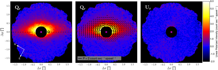
Figure 1. Left: the β Pic debris disk in polarized intensity, Qr, from observations with GPI's polarimetry mode. The disk image has been rotated so that the midplane of the outer disk (PA = 291; black dashed horizontal line) is horizontal. The star's location and β Pic b's location are marked by the magenta × and black circle, respectively. Center: the Qr image with polarization vectors overplotted. Though the centrosymmetric nature of the polarization is captured in the transformation to the radial stokes images, the vectors serve to emphasize this behavior. Right: the radial polarized intensity, Ur, from the same datacube as the image on the left, shown at the same color scale. For optically thin circumstellar material, the flux is expected to be solely in the Qr image, thus this images provides an estimate of the noise in the disk image.
Download figure:
Standard image High-resolution image2.2. Spectral Mode Observations
Observations of β Pic in spectroscopic mode (spec. mode) were carried out during four separate GPI commissioning runs, as well as during an ongoing astrometric monitoring program scheduled during regular general observing time. In total, we present nine individual sets of observations over seven epochs (Table 1). Two of the observation sets have been previously published: the H-band data set from 2013 November 18 (Macintosh et al. 2014) and the J-band data set from 2013 December 10 (Bonnefoy et al. 2014). Here we have re-reduced all the data in a consistent manner in an effort to reduce systematic biases and maximize the homogeneity of the data set. As with the polarization mode observations, those observations that were taken during the instrument's commissioning were carried out during AO optimization tests and therefore have a range of exposure times and filter combinations.
All data sets were reduced with standard recipes provided by the GPI DRP. Raw data frames were dark subtracted and destriped for microphonics in the same manner as the polarimetry observations. A short-exposure arc lamp image was taken contemporaneously with each science observation to measure the offsets of the lenslet spectra due to flexure within the IFS. The mean shift was calculated for a subset of lenslets across the field of view relative to a high signal-to-noise ratio (S/N) arc lamp image taken at zenith via a Levenberg–Marquardt least-squares minimization algorithm (Wolff et al. 2014).
The raw detector image was then transformed into a spectral datacube, using a box extraction method. For observations obtained with the K1 and K2 filters, thermal sky observations were taken immediately before or after the observation sequence. Sky background cubes were created in the same manner described above and subtracted from science datacubes. Finally, all cubes were corrected for distortion (Konopacky et al. 2014).
Each data set was PSF subtracted using the methods outlined in Pueyo et al. (2015). To minimize systematic biases, the ensemble of data sets was treated as uniformly as possible. The main steps of this data reduction process include: high-pass filtering, to remove the remaining PSF halo; wavelength-to-wavelength and cube-to-cube image registration, to correct for atmospheric differential refraction and sub-pixel stellar motion across the observing sequence; subtracting the speckles using the KLIP principal component analysis algorithm (Soummer et al. 2012) on each wavelength slice in each cube; rotation to align the north angle of each image; and co-adding the resulting cubes in time.
For the epochs in which β Pic b was observed on consecutive nights, relative alignment was tested using both the cross-correlation method described in Pueyo et al. (2015) and the absolute stellar locations based on the satellite spot centroids derived using the GPI DRP. For these epochs we found better consistency in the location of β Pic b using the DRP centroids, which we then chose to adopt for all data sets.
The KLIP algorithm was implemented using both spectral differential imaging (SDI; Marois et al. 2000) and ADI, building for each slice a PSF library that takes advantage of the radial and azimuthal speckle diversity (in wavelength and in PA, respectively). Due to the relative brightness of β Pic b with respect to the neighboring speckles we limited the exploration of KLIP parameter space to two zone geometries and two exclusion criteria (1 and 1.5 PSF FWHM) for each data set. For each slice, the 30 PSFs that were the most correlated in the region where β Pic b is located were used for PSF subtraction, except for the J-band data which required 50 PSFs for satisfactory subtraction.
To determine the optimal number of principal components to use for each data set, we examined both the evolution of the extracted spectrum and the astrometric stability as a function of wavelength as we increased the number of components. This latter test helps us to rule out the pathological cases for which either a residual speckle (i.e., insufficiently aggressive PSF subtraction) or self-subtraction (i.e., over-aggressive PSF subtraction) bias planet centroid estimates. We checked for potential biases by comparing astrometric positions measured when using only a high-pass filter with those measured when applying KLIP. Finally, we checked for self-consistency by injecting six synthetic point sources at the same separation as β Pic b, but at different PAs. Based on these tests we concluded that the astrometric measurements do not feature systematics either introduced by residual speckles or biases associated with KLIP above the uncertainty levels reported in Section 4.1.
3. DISK RESULTS
The debris disk is recovered in polarized light from ∼17 (32 AU), to an inner working angle of ∼032 (6.4 AU); see Figure 1. While GPI's H-band focal plane mask extends to a radius of ∼012, uncorrected instrumental polarization and other noise sources dominate over the disk emission at separations smaller than ∼032.
A comparison of the Qr and Ur images indicate that the disk is detected at a high S/N out to the edge of the GPI field. Overplotting linear polarization vectors indicates that the emission is linearly polarized perpendicular to the scattering plane, as expected for optically thin conditions. This property is captured in the transformation to radial Stokes parameters, but we have included the vectors in Figure 1 for additional clarity.
Morphologically, the disk appears vertically offset from the midplane of the outer disk in the NW direction, indicative of a slight inclination relative to the line of sight. This is consistent with previous models of the disk at similar angular separations (e.g., Milli et al. 2014).
The Ur image shows low level structure in the form of a dipole-like pattern with positive emission in the E–W direction. Figure 2 displays the Ur image with a color scale that emphasizes this structure. In the radial Stokes basis, this is the pattern produced by a constant linear polarization across the field, which could be associated with residual instrumental polarization that was not successfully subtracted during the data reduction process. Since the level of these residuals is much lower than the disk emission, we defer improvement of our instrumental polarization subtraction procedure for future work.
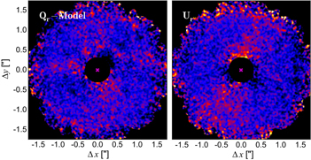
Figure 2. Left: the residuals of the Qr image after subtraction of the best-fit disk model, shown at a stretch to emphasize their structure. The residual structure in the NW–SE direction is likely due imperfect subtraction of the instrumental polarization, but may also represent the difference between the true scattering properties of the grains and the Henyey–Greenstein function used in the model. Right: the Ur image, shown at the same stretch as the residuals. The star's location is marked with a magenta ×.
Download figure:
Standard image High-resolution imageThe disk is not detected in total intensity (Stokes I; Figure 3), where images are dominated by the residual uncorrected PSF of the star itself. Due to both the extended nature of the disk at these angular scales and frame-to-frame variation of the PSF (compounded by the AO tests carried out during the observing sequence), ADI PSF subtraction has proven unsuccessful. Without an unbiased total intensity image of the disk, characterization of the polarization fraction remains out of reach at present. As a result, we opt to model only the polarized intensity.
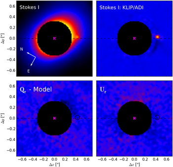
Figure 3. Top left: the Stokes I image from the polarimetry observations, without PSF subtraction. The dashed line indicates the position angle of the outer disk. The planet can be seen at a separation of ∼04 just above the horizontal line, to the SW from the central star. Top right: the Stokes I image after applying KLIP/ADI PSF subtraction. The planet is recovered at a very high S/N. Bottom left: the polarized intensity image, Qr, after disk model subtraction. The black circle indicates the location of the planet in the Stokes I images. Bottom right: the radial Stokes image (same as in Figure 1), Ur. No point source polarization signal is detected for β Pic b in either Stokes Qr or Ur. All images have been rotated so that the outer disk's PA is horizontal (dashed black line). In all four images the star's location is marked with a magenta ×.
Download figure:
Standard image High-resolution image3.1. Disk Modeling
The principal objective of our disk modeling is to retrieve basic geometric properties of the disk. The modeling approach adopted here is to combine a simple recipe for the 3D dust density distribution with a parametric model of the polarized scattering phase function and then fit to the data using the affine-invariant sampler in a parallel-tempering scheme from the emcee Markov chain Monte Carlo (MCMC) package (Foreman-Mackey et al. 2013). Parallel tempering uses walkers at different "temperatures" to broadly sample the posterior distributions and is therefore a useful strategy when the likelihood surface is complex.
For a disk seen in edge-on projection, the radial dust density distribution becomes degenerate with the dust scattering properties. This degeneracy is typically broken with the use of physical grain models, which describe scattering properties (including polarization) as a function of wavelength. In practice, observations are fit to grain models either using simultaneous polarization and total intensity information (e.g., Graham et al. 2007), or multicolor images (Golimowski et al. 2006). With only single wavelength polarized intensity images available, we instead use the HG scattering function (Henyey & Greenstein 1941) to describe the scattering efficiency as a function of scattering angle. The shape of the HG scattering function is a function of only one parameter, the expectation value of the cosine of the scattering angle,  and thus provides a useful tool to approximate grain scattering when using physical models is impractical. The applicability of the HG scattering function to the modeling of our polarized intensity images is discussed in Section 5.1.
Our dust density model, expressed in stellocentric coordinates,  follows a power law between an inner radius, R1, and an outer radius, R2, and has a Gaussian vertical profile with rms height
  and constant aspect ratio, h0:
where r is the radial distance from the star, z is the height above the disk midplane and β is the power law index of the dust density. Inside R1 and outside R2 the dust density is zero. The dust density distribution is combined with the HG function,  to generate a scattered light image of the disk as seen in 2D projection from the observer's frame, where the intensity for a given pixel
  is calculated as the integral along the line of sight direction
Here,  represents the dust density distribution, but tilted with a disk inclination, ϕ, relative to the observer's line of sight. The scattering angle
  is a function of position.
The  term accounts for the diminishing stellar flux as a function of distance from the star. The disk's PA,
  is implemented as a coordinate transformation between the stellocentric coordinates and the projected observer's coordinates. The constant, I0, and the flux normalization, N0, have been included to account for any possible biases and the conversion between model flux and detector counts, respectively. In summary, our model has a total of nine free parameters:
Within the current model there exists a degeneracy between forward scattering ( ) with an inclination of
  and backwards scattering (
 ) with an inclination of
  In an effort to conserve computation time we chose to assume forward scattering and place a prior constraint on the scattering parameter,
  which is consistent with the model of Milli et al. (2014). A summary of the model parameters and their prior distributions can be found in Table 2.
Table 2. Disk Model Parameters
| Parameter | Symbol | Range | Prior Distribution |
|---|---|---|---|
| Inner Radius | R1 | 1–100 AU | Uniform in 
|
| Outer Radius | R2 | R1–500 AU | Uniform in 
|
| Density Power Law Index | β | 0.5–4 | Uniform in β |
| Scale height aspect ratio | h0 | 0.01–2 | Uniform in 
|
| HG asymmetry parameter | g | 0–1 | Uniform in g |
| Line of Sight Inclination | ϕ | 80°–90° | Uniform in 
|
| Position Angle |

|
25°–35° | Uniform in 
|
| Flux Normalization | N0 | 1–1000 | Uniform in 
|
| Flux Offset | I0 | −5–10 | Uniform in I0 |
Download table as: ASCIITypeset image
We fit the model to the GPI disk image using the parallel-tempering sampler from the emcee package. The diffraction limit in the H-band for Gemini south is 0043, equal to about three GPI pixels. We therefore apply a 3 × 3 pixel binning to both the Qr and Ur images before fitting. This improves the noise statistics and speeds up the execution time of the MCMC fit, without significantly sacrificing spatial information. At each angular separation in the Qr image, the errors were estimated as the standard deviation of a 3 pixel-wide annulus centered at that separation in the Ur image. The error estimates therefore contained photon noise, read noise and the unsubtracted instrumental polarization.
The MCMC sampler was run for 2500 steps with 2 temperatures, 128 walkers and burn-in of 500 steps. Additional temperature chains were not employed because of the additional computational cost incurred and the lack of evidence that the Markov chain sampler was only selecting local islands of high likelihood. One strength of using ensemble sampling over other types of sampling for MCMC fitting is that large speed-ups are possible via parallel-processing. On a 32-core (2.3 GHz) computer the entire MCMC run took nearly five days to complete.
After the run, the maximum auto-correlation across all parameters was found to be 85 steps, indicating that the chains should have reached equilibrium (Foreman-Mackey et al. 2013 recommend  autocorrelation times for convergence). In addition, the chains were examined by eye and appeared to have reached steady-state by the end of the burn-in phase. The posterior distributions (Figure 4) were estimated from the zero temperature walkers, using only one of out every 85 steps to ensure statistical independence of the surviving samples. The expected covariance between the inclination ϕ and g (Kalas & Jewitt 1995) is reproduced. Degeneracies are also found between ϕ and g, h0 and g, h0 and β, h0 and ϕ, β and g, and β and ϕ, but in all cases, the parameters appear to be well constrained.
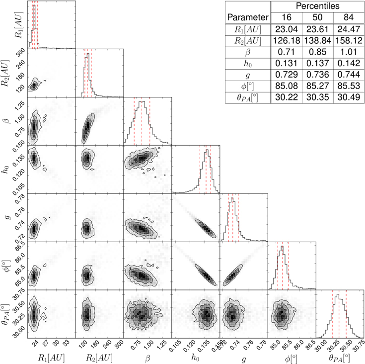
Figure 4. Posterior distributions of the model parameters from MCMC disk model fitting to the Qr disk image. The diagonal histograms show the posterior distributions of each parameter marginalized across all the other parameters. In each plot, the dashed lines indicate the 16%, 50%, and 84% percentiles. The off-diagonal plots display the joint probability distributions with contour levels at the same percentiles. The normalization term, N0, and the constant offset term, I0, have been excluded from this plot because they convey no relevant astrophysical information. Inset table: the 16%, 50%, and 84% percentiles from the marginalized distributions.
Download figure:
Standard image High-resolution imageThe 16%, 50%, and 84% percentiles for each parameter are displayed in a table in the upper right corner of Figure 4. Marginalized across all parameters we find a disk inclined relative to the line of sight by  with an inner radius of
  , an outer radius of
  and an aspect ratio of
  The PA of the disk is
  where the errors include GPI's systematic error in PA (∼02). Note that the systematic uncertainty in the PA is not reflected in Figure 4. The dust is well fit by forward scattering grains, with a scattering asymmetry parameter of
  These results are further discussed in Section 5.1.
Figure 5 displays the best fit model and the residuals of the Qr image minus the model. The best fit model was generated using the median value of each parameter in the marginalized posterior distribution. We find that the highest likelihood disk model successfully reproduces the GPI data. When examined at a different color scale, the residuals image displays similar low-level structure as that of the Ur image (Figure 2). The structure in the NW–SE direction is likely the Qr counterpart of the residual instrumental polarization that's seen in the Ur image. A possible alternative explanation is that the structure could be due to a mismatch between the true scattering properties of the dust and the HG scattering function at small angular separations. A second structure can be seen along the disk midplane to the NE of the star. This asymmetric brightness feature is possibly due to a local overdensity of dust, that would increase the scattering at that location. Indeed, the β Pic disk is known to have multiple brightness asymmetries (Apai et al. 2015 provide a good summary). However, the feature is detected at similar brightness levels as the residual instrumental polarization and may yet be an uncharacterized artifact of the polarimetry reduction. Deeper observations of the disk will be required to distinguish between a true brightness asymmetry and instrumental effects.
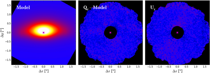
Figure 5. Left: the disk model generated with the median values from the marginalized posterior distributions (as found in Figure 4). The inner edge of the disk is at a projected separation of 12, but contributes negligible light to the observed surface brightness. Center: the residuals of Qr image minus the disk model. The level of the residuals is very similar to the Ur image. Right: the Ur image, reproduced here as a point of comparison to the residual image. In all images the star's location is marked with a magenta ×. The images have been rotated so that the outer disk is horizontal and all are displayed at the same color scale as Figure 1.
Download figure:
Standard image High-resolution image4. PLANET RESULTS.
4.1. Astrometry in Spectroscopy Mode
We describe here in broad terms our astrometric measurements and estimation of uncertainties, without delving into the details of each individual data set. For each epoch, the entirety of the data set is combined to estimate the planet's position relative to β Pic. The errors on this relative position are a combination of the error on the star's position, the planet's position, GPI's pixel scale and the accuracy to which we know GPI's orientation relative to true North.
For each data set, the stellar position was calculated using two methods. The wavelength slices of each datacube were first registered using the relative alignment procedure described in Section 2.2 and then collapsed into a broadband image. A Radon transform was then performed on the radially elongated satellite spots to find the stellar position (as in Pueyo et al. 2015). The stellar position was also estimated using the geometric mean of the satellite spot locations provided by the GPI DRP. Most H-band data sets show agreement between two methods at the 0.05 pixel level, with the exception of the 2013 December 11 commissioning sequence, during which extensive AO performance tests where being carried out. For K-band data sets the difference between the two methods is no more than 0.05 pixels and for the J-band data set it is 0.2 pixels. We found greater consistency in the relative location of β Pic b between observations obtained on consecutive nights when using the Radon method, and therefore chose to adopt the centroids measured with the Radon method for all measurements. For each data set, we considered the difference between the two methods as our estimate for the uncertainty on stellar position.
The location of β Pic b (in detector coordinates) was estimated at each wavelength channel, at each epoch and in each filter using the modified matched filter described in Pueyo et al. (2015). The uncertainty in β Pic b's location was estimated as the scatter in the position of the planet as a function of wavelength and number of principal components. We found the uncertainly to range from 0.05 pixels, for the data sets with significant field rotation and where the planet was at larger separations, up to 0.15 pixels, for the later epochs where the planet is significantly closer to the stellar host and SDI is less effective.
We estimated GPI's pixel scale using the methods described in Konopacky et al. (2014) by combining all the data presented therein with four new observations of  Ori B, taken between 2014 September and 2015 January. We find an updated pixel scale value of 14.13 ± 0.01 mas/lenslet. Konopacky et al. (2014) measured a PA offset of −100 ± 003 during GPI commissioning. Subsequently, version 1.2 of the GPI DRP was updated to incorporate that 1° offset and correct for it automatically. Using the new measurements of
  Ori B, we find a residual PA offset of −011 ± 025.
Based on the measured location of β Pic b and its parent star in detector coordinates we calculated the relative separation and PA at each epoch. The separation was converted to milliarcseconds using the new platescale estimate and the PA was adjusted by  The separation and PA from each measurement can be found in Table 1. Uncertainties on these quantities were combined with the errors on the star position and planet position to yield the errors presented in the table.
4.2. Astrometry in Polarimetry Mode
β Pic b is detected in the Stokes I image as a point source superimposed on the extended PSF halo (Figure 3). After applying PSF subtraction using a python implementation of KLIP/ADI (Wang et al. 2015) to the image, the planet is recovered at extremely high S/N. The planet's position in the Stokes I image was estimated using the StarFinder IDL package (Diolaiti et al. 2000), which requires the user to input a PSF model for precision astrometry. In GPI's polarimetry mode the entire bandpass is seen by each frame and therefore the satellite spots are elongated and cannot be used as a PSF reference, as they are in spectroscopy mode. Instead, we used a GPI PSF generated with AO simulation software (Poyneer & Macintosh 2006).
To estimate astrometric errors we used StarFinder to measure β Pic b's location in the total intensity image from each of the 49 polarization data cubes. The rms difference between the planet location in the individual cubes and the Stokes I image was taken to be the error in the planet location. The error on the location of the star is estimated from the rms scatter of the measured star's position across the set of cubes. This error tracks the motion of the star behind the coronagraph between frames, which we expect to be larger than the errors on the star's position determined by the Radon transform, and therefore likely overestimates the errors.
The position of β Pic b in the polarimetry mode observations can be found in Table 1. As with the spectroscopy mode data, the errors represent a combination of the errors on the star's and planet's positions, GPI's pixel scale and GPI's PA offset on the sky.
4.3. Orbit Fitting
Using the ten newly obtained astrometric points (nine from spec. mode and one from pol. mode), combined with the data sets presented by Chauvin et al. (2012) and Nielsen et al. (2014), we fit for the six Keplerian orbital elements of β Pic b plus the total mass of the system using the parallel-tempered sampler from emcee (Foreman-Mackey et al. 2014). While astrometric datapoints have been published in other papers, in an effort to minimize systematics between data sets, we limited ourselves to only these two large data sets where considerable effort has been made to calibrate astrometric errors. The fitting code was previously used in Kalas et al. (2013), Macintosh et al. (2014), and Pueyo et al. (2015). We also fit the radial velocity measurement of the planet from Snellen et al. (2014), which allows us to constrain the line of sight orbital direction and break the degeneracy between the locations of the ascending and descending node.
The model fits seven parameters: the semimajor axis, a; the epoch of periastron, τ; the argument of periastron, ω; the PA of the ascending node, Ω; the inclination, i; the eccentricity, e; and the total mass of the system, MT. Our orbital frame of reference followed the binary star sign convention used in Green (1985). Under this convention the ascending node is defined as the location in the orbit where the planet crosses the plane of the sky (centered on the star), moving southward in projection. Note that this is 180° different from the convention used in Chauvin et al. (2012). The projected PA of the ascending node on the sky is defined from north, increasing to the east. The argument of the periastron is defined as the angle between the ascending node and the location of the periastron in the orbit, with ω increasing from the ascending node. The epoch of periastron, τ, is defined in units of orbital period, from 1995 October 10 (Julian date 2450000.5). A summary of the orbital parameters and their prior distributions can be found in Table 3.
Table 3. Orbit Model Parameters
| Parameter | Symbol | Range | Prior Distribution |
|---|---|---|---|
| Semimajor axis | a | 4–40 AU | Uniform in 
|
| Epoch of Periastron | τ | −1.0–1.0 | Uniform in τ |
| Argument of Periastron | ω |
 rad rad |
Uniform in ω |
| Position Angle of the Ascending Node | Ω | 25°–85° | Uniform in Ω |
| Inclination | i | 81°–99° | Uniform in 
|
| Eccentricity | e | 0.00001–0.99 | Uniform in e |
| Total Mass | MT | 0–3 M⊙ | Uniform in 
|
Download table as: ASCIITypeset image
The MCMC sampler was run for 10,000 steps with 10 temperatures and 256 walkers after a "burn-in" of 2000 steps. After the run, the maximum auto-correlation across all parameters was found to be 25 steps, indicating that the chains should have reached equilibrium. The posterior distributions (Figure 6) were estimated using the zero temperature walkers, using only one of out every 25 steps. In Figure 6, the epoch of periastron was wrapped around to be only positive between 0 and 1 and the arguments of the periastron was wrapped around to range from 0° to 360°. A random selection of 500 accepted orbits are plotted on top of the astrometric and radial velocity datapoints in Figures 7 and 8, respectively. While the orbital fits are generally consistent with most of the astrometric datapoints, the majority of the orbital solutions fall more than 1σ from the measured radial velocity.
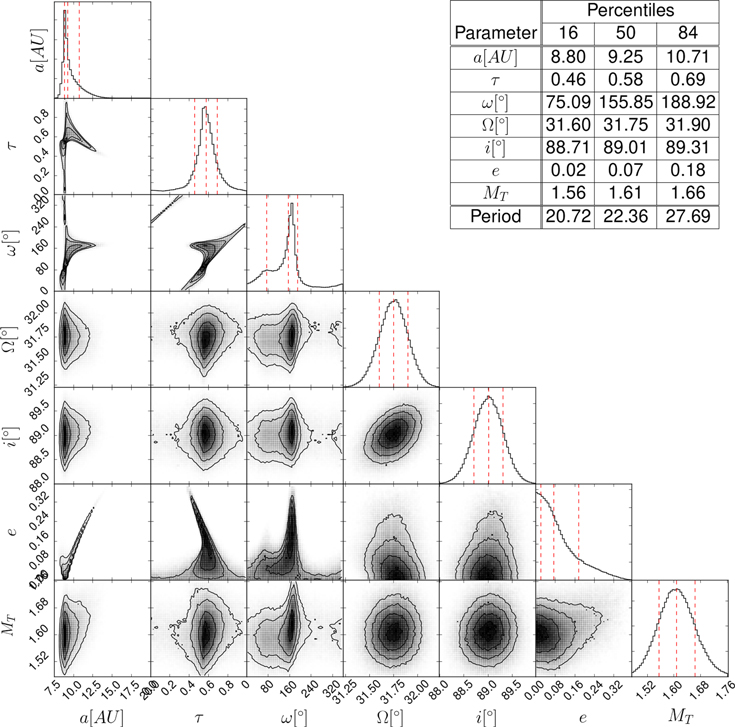
Figure 6. Posterior distributions of the model parameters from the MCMC orbit model fitting to the astrometry data points, as well as the radial velocity value from Snellen et al. (2014). The diagonal histograms show the posterior distributions of each parameter marginalized across all the other parameters. In each plot, the red dashed lines indicate the 16%, 50%, and 84% percentiles. The off-diagonal plots display the joint probability distributions with contour levels at the same percentiles. Inset table: the 16%, 50%, and 84% percentiles from the marginalized distributions.
Download figure:
Standard image High-resolution image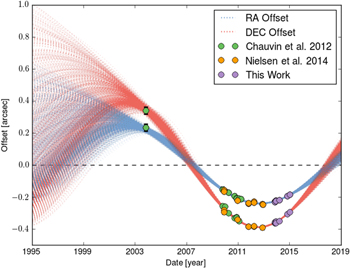
Figure 7. R.A. (blue) and decl. (red) offsets of β Pic b from β Pic for a random selection of 100 accepted orbits (dotted lines) from the MCMC run. The 29 data points used in the fit are overplotted, with the colors indicating their source. Error bars on the datapoint are smaller than the markers, except for the 2003 measurement from Chauvin et al. (2012). This fit includes the radial velocity constraint from Snellen et al. (2014) shown in Figure 8.
Download figure:
Standard image High-resolution image
Figure 8. Predicted radial velocity of β Pic b from from the orbital fit constrained by the astrometric data plotted in Figure 7 and the single radial velocity measurement from Snellen et al. (2014) (point with error bar). A random selection of 100 accepted orbits (purple dotted lines) from the MCMC are shown.
Download figure:
Standard image High-resolution imageWe find that the planet has a semimajor axis of  , an inclination of 8901 ± 030, and an ascending node at a PA of 3175 ± 015. We take the median of the marginalized posterior distribution to be the best estimator of each parameter's value, and the 68% confidence values as the errors. Following this convention, the eccentricity of the orbit is found to be
  However, the eccentricity is a positive definite quantity and typical estimators (e.g., the mean and median) will overestimate the true eccentricity when it is small (
 ). When considering eccentricities of radial velocity planets, Zakamska et al. (2011) consider several different estimators and find that for small eccentricities the mode of the distribution is the least biased. The mode of our distribution falls in the smallest eccentricity bin indicating an eccentricity very close to zero. Therefore, it is perhaps more appropriate to quote the upper limit on the eccentricity
  (95% confidence).
For orbits with higher eccentricities ( ), the epoch and argument of periastron have strong peaks at ∼0.5 periods and
  respectively. At lower eccentricities these two parameters remain degenerate, with a large range of acceptable values. Overall, the marginalized distributions reveal that these parameters are still relatively unconstrained. The ensemble of accepted orbits at the end of the run have a reduced
  of
of 
Marginalized across all parameters, the total mass of the system is 1.61 ± 0.05 M⊙. At  β Pic b contributes less than 1% to the total mass, giving β Pic itself a mass of
  This falls slightly below the range estimated by Crifo et al. (1997) (1.7–1.8M⊙) and just within the range of Blondel & Djie (2006) (1.65–1.87 M⊙), who both use evolutionary models and the HR diagram to date β Pic. This estimate provides a slightly smaller value than that presented in Nielsen et al. (2014), though still consistent within their errors (
 )
)
By combining the semimajor axis and stellar mass values of each walker at each accepted iteration, we are able to create a posterior distribution for the orbital period, from which we derive that  . The large upper limit is due to the extended tail in the semimajor axis distribution.
4.4. Planet Polarization
Giant exoplanets may have polarized emission in the NIR either due to rotationally induced oblateness (Marley & Sengupta 2011) or asymmetries in cloud cover (de Kok et al. 2011). For β Pic b, the recently measured rotational period of ∼8 hr would induce a polarization signature due to oblateness of less than 0.1% (below GPI's current sensitivity limit, Wiktorowicz et al. 2014). Therefore, any detected polarization signal would be indicative of cloudy structure.
To estimate β Pic b's polarization, we first created a disk-free linear polarized intensity image by combining the model-subtracted Qr image with the Ur image ( ). The total polarized flux at the location of β Pic b, within an aperture of radius
  was then compared to the flux of 38 independent apertures at the same angular separation. We find that β Pic b's polarized flux is
  from the mean flux of the independent apertures, consistent with zero linear polarization signal from the planet (see Figure 3). While this measurement does not provide any evidence for cloud structure, it does not exclude the possibility either; the magnitude of cloud-induced polarization depends on many factors, including the atmospheric temperature and pressure profile, the composition, the nature of the inhomogeneities, rotation, and viewing angle. The PSF variability during the observations makes accurate recovery of the total intensity of the planet difficult, and thus we leave the characterization of an upper limit on the planet's polarization fraction for future work.
5. DISCUSSION.
5.1. The Debris Disk
With GPI we probe the projected disk between 03 and 17 at high spatial resolution. The work presented here has two advantages over previous attempts to model the disk at similar angular separations. First, the polarized intensity images provide a unique view of the disk, in particular the vertical extent is free of any biases associated with ADI PSF subtraction. Second, the MCMC fitting allows us to fully explore the multi-dimensional parameter-space and place quantitative confidence intervals on the model parameters.
MCMC fitting requires evaluation of the likelihood function for each set of parameters that is examined. The cost of fitting depends on the computational expense of evaluating the model and the dimensionality of the model parameter space. For that reason we have limited our exploration to optically thin scattering, an analytic recipe for the phase function, and a simple model of the dust distribution. We do not consider multi-component disks (as modeled for the outer disk, e.g., Ahmic et al. 2009) and we assume that the disk aspect ratio is constant. Regardless of these simplifications, we find that this model provides an excellent fit to our polarized image.
The HG scattering function is often used to model the total intensity scattering efficiency of dust grains, but has not been used extensively for polarized intensity. This is at least partially due to the fact that in most circumstances where polarized intensity is measured, total intensity is obtained as well, allowing for more sophisticated modeling of the dust scattering. In addition, the scattering efficiency of polarized intensity of small spherical particles approaches zero at very small scattering angles, a feature that is not captured by the HG function. While the exact shape of the HG function cannot fully reproduce the polarized scattering efficiency function for physical models, a quick informal survey of possible grain models indicates that our best fit  can be reproduced by Mie scattering particles with a radius of ∼1 μm and an index of refraction of m = 1.033–0.01i, similar to the porous, icy grains inferred by Graham et al. (2007) for AU Mic. However, as previously mentioned, a true characterization of the physical grain scattering properties will require either an unbiased total intensity image, or polarized intensity images at other wavelengths. We leave the characterization of the dust properties of the inner disk for future work.
The observations of Milli et al. (2014) have a field of view (04–38) that overlaps with our disk detection and therefore provide a good point of comparison. They model the L' emission with a single component disk model similar to ours, albeit with different radial and vertical dust density profiles. Even so, their best fit inclination (i = 86°) and PA ( ) agree fairly well with our own. Their data set constrains the sky-plane inclination less precisely and inclinations of 85°–88° provide good fits to their data. The consistency between their measurements and ours builds confidence that the measured angles are not highly sensitive to the assumed scattering properties and radial dust distribution. The PA of the disk seen in our images (
 ) and those of Milli et al. (2014) appears to be misaligned from both the outer main disk (
 Apai et al. 2015) and the warp (
 ). This offset, and how our disk images fit into the context of the whole system, will be further discussed in Section 5.3.
The results of our model fitting reveal an inclined disk with an inner radius of  (12), populated by grains that preferentially forward scatter polarized light. The majority of the detected polarized flux is therefore inside the projected inner radius and the result of forward scattering by the constituent dust grains. Without direct detections of either the inner or outer radius, the constraints on both are governed by the overall shape and spacing of isophotal contours (see Figure 9).
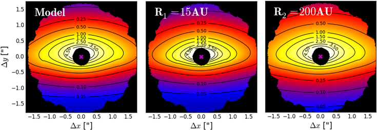
Figure 9. Three different disk models with polarized intensity contours overplotted. The differences in the shapes and spacing of the contours illustrate how the inner and outer radius are constrained even though neither are directly detected. All three images are displayed with the same Log color scale. This color scale has been chosen to emphasize the differences between the models, and is not the same scale as Figures 1 and 5. Left: the best fit disk model from Figure 5. Center: the same disk model with the inner radius changed from the median value of R1 = 23.6 to 15 AU. The smaller inner radius increases the scattering contributions from dust at smaller projected separations. As a result, the spacing of the inner contours, in particular in the horizontal direction, becomes tighter while leaving the outer contours relatively unchanged. In addition, the contour ansae are pulled down toward midplane. Right: the best fit disk model with the outer radius changed from R2 = 138 to 200 AU. The larger outer radius increases the scattering contributions from dust at separations further above the midplane, which pushes the contours further out in the vertical direction.
Download figure:
Standard image High-resolution imageThe location of the inner edge of the disk seen in our model is a unique feature of this work and has not been found in previous scattered light imaging at similar angular separations. This could be attributed to both the scattering properties of the dust, which make the inner edge difficult to see, and the modeling strategies used in those studies. Milli et al. (2014) also use a HG function to model their dust. However, their model considers a population of parent bodies between 50 AU and 120 AU, with the density falling as separate power laws inside and outside of these radii and they do not define an inner radius in the same manner as in our model. Apai et al. (2015) make surface brightness measurements of the disk between 05 and 150, but find no noticeable change in the brightness profile at 11. In our model, we find that the forward scattering nature of the dust grains means that the inner edge itself contributes minimally to the observed surface brightness at its projected separation. This serves to emphasize the critical role of dust scattering when interpreting the surface brightness as a function of radius; a smooth surface density by itself does not necessarily exclude features in the radial dust profile.
Note that our model has been defined with a sharp cut-off inside the inner radius, and caution should be used when interpreting the exact value. There may be dust inside of the inner radius with a lower surface density. For example, the true dust density inside the inner radius may have a slowly decreasing inner power-law, such as those considered in Milli et al. (2014).
Imaging and spectroscopic studies in the mid-IR have probed similar regions of the debris disk at wavelengths where contrast between the stellar flux and the dust (thermal) emission is more favorable than in the optical and NIR. Okamoto et al. (2004) found spectroscopic evidence for dust belts at 6, 16, and 30 AU. Wahhaj et al. (2003) fit a series of four dust belts to deconvolved 18 μm images and found their best fit radii to be 14, 28, 52, and 82 AU. With the exception of the belts close to ∼15 AU, all of these belts are either well outside or at the very edge of our field of view. The 6 AU belt seen by Okamoto et al. (2004) is below our inner working angle. We note that the Okamoto et al. (2004) belt at ∼16 AU only occurs on the NE side, at roughly the same location as the tentative brightness asymmetry seen in our disk model residuals. We see no evidence of the other belts in projection, but we model the disk with a continuous dust distribution and therefore may not be sensitive to dust at their locations. Mid-IR imaging by Weinberger et al. (2003) indicates emission within 20 AU that is significantly offset in PA from the main outer disk. In our disk image we see no indication of this offset.
Previous studies of β Pic's debris disk in polarized scattered light have been carried out both in the optical (Gledhill et al. 1991; Wolstencroft et al. 1995) and the NIR (Tamura et al. 2006). These observations image the disk at separations of 15''–30'' and 26–64, in the optical and NIR, respectively. At these angular separations the total intensity observations are not limited by the PSF halo and when combined with the polarized images, polarization fraction can be used to model the dust grains (Voshchinnikov & Krügel 1999; Krivova et al. 2000). Tamura et al. (2006) combine the optical measurements with their K-band data and find that the observations could be explained by scattering from fluffy aggregates made up of sub-micron dust grains. Unfortunately, the lack of total intensity images and a non-overlapping field of view make a direct comparison between our observations and this past work difficult.
5.2. β Pic b
In general, our orbit fit is consistent with those previously published (e.g., Chauvin et al. 2012; Macintosh et al. 2014; Nielsen et al. 2014), but the longer temporal baseline and increased astrometric precision significantly tighten the constraints on the orbital parameters. In particular, we find that the PA of the ascending node of the planet lies in between the main outer disk and warp feature, consistent with Nielsen et al. (2014).
At first glance, the errors on our orbital elements appear comparable to those in Macintosh et al. (2014). However, our fit includes the total mass of the system as an additional free parameter. Nielsen et al. (2014) modeled the system's total mass as a free parameter in their orbital fit and found that accounting for the uncertainty in the system's total mass resulted in larger uncertainties in the planet's orbital elements. In particular, they find that with a floating system mass the eccentricity distribution has a long tail that peaks at high eccentricities. Due to a degeneracy between semimajor axis and eccentricity, this stretched the semimajor axis distribution to higher values as well. In Figure 6, we find that the eccentricity is now significantly better constrained ( ), and while the degeneracy remains, the semimajor axis is constrained to be
  with 84% confidence.
For each orbit defining our posterior distribution, we calculate the epoch of closest approach and find that it will fall between 2017 November 20, and 2018 April 4 with 68% confidence. With our derived inclination of i = 8901 ± 036, the updated transit probability is ∼0.06%, assuming that the planet will transit if the inclination is within 005 from 90°. This is a reduction by a factor of ∼50 from the estimate in Macintosh et al. (2014), who found i = 90.7 ± 0.7.
Even though the likelihood of a planet transit is small, it is still possible that dust particles orbiting within the planet's Hill sphere ( AU) will transit. Indeed the transit of a ring system surrounding an exoplanet was recently detected around J1407 (Mamajek et al. 2012). In the outer solar system, satellites around the giant planets have stable orbits within a Hill sphere about the planet out to
  when in prograde orbits and
  in retrograde orbits (Shen & Tremaine 2008). For β Pic b, assuming a planetary mass of 11 MJ, a semimajor axis of 9.25 AU, a circular orbit and a stellar mass of 1.60 M⊙, we calculate a Hill radius of ∼1.2 AU. Thus, stable orbits within the Hill sphere will transit if the planet's inclination is within 38 and 53 of edge-on, for prograde and retrograde orbits, respectively. Our new constraints on the inclination indicate that these orbits will almost certainly transit. However, the true transit probability will depend not only on the exact location of the dust, but also its orientation relative to the observer. For example, dust that fills the stable orbits and is orbiting face-on relative to the observer will transit, but if it is orbiting edge-on it will not.
The presence of infalling comets (a.k.a. falling evaporating bodies, or FEBs) has been previously inferred by redshifted absorption features in β Pic's spectrum (Beust & Morbidelli 1996). Thébault & Beust (2001) suggested that a massive ( ) planet within ∼20 AU on a slightly eccentric orbit (
 ), could be responsible for imparting highly elliptical orbits on bodies within a 3:1 or 4:1 resonance, that then plunge toward the star. In this scenario the argument of the periastron of the planet is restricted to a value of
  from the line of sight. Using our definitions, the equivalent requirement is
  Our results neither confirm nor rule out the infalling comet scenario. While the marginalized distribution of the argument of periastron allows for a broad range of values, if the orbit is indeed eccentric, then ω peaks strongly around 170°, just outside of the acceptable values for this scenario. Thébault & Beust (2001) find that if the eccentricity of the massive perturber (here assumed to be β Pic b) is as large as
  then the infalling comets most likely originate in the 3:1 resonance, which occurs between 18 and 22 AU based on our 68% confidence range for β Pic b. The inner edge of the dust in our scattered light images falls at
  , outside of range of values for the 3:1 resonance. However, as noted above, our inner radius is sharply defined, and there may still be material inside. For smaller perturber eccentricities the infalling comets originate in the 4:1 resonance, which occurs between 22.2 and 26.5 AU. Our disk model does not constrain whether there is an excess of bodies librating in the 4:1 resonance.
5.3. The Disk–Planet Interaction
A planet on an inclined orbit is thought to be responsible for the warp feature in the region of the disk outside our field of view at ∼80 AU (Mouillet et al. 1997; Augereau et al. 2001). The directly imaged planet β Pic b (Lagrange et al. 2009) has a mass, semimajor axis, and inclination consistent with producing the warp (e.g., Dawson et al. 2011). The updated PA of β Pic b's ascending node,  is offset by 265 with respect to the flat outer disk (291 ± 01; Apai et al. 2015), consistent with producing a warp tilted by 5° counter-clockwise with respect to the flat outer disk. As illustrated by Apai et al. (2015, Figure 21), our azimuthal viewing angle of the warped disk affects the degree to which the inner disk and the planet's orbit appear aligned with the flat outer disk in projection and also affects the projected height of the warp. Although the planet's updated orbit remains consistent with sculpting the outer regions of disk, several features of the inner regions of the disk that we measured here are unexpected solely from sculpting by β Pic b (Figure 10).
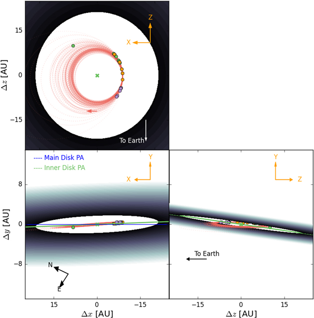
Figure 10. Three orthogonal projections of the system: the plane of the sky (bottom left), a top down view (top left), and a side view (bottom right). The system has been rotated in three dimensions so that the midplane of outer disk is horizontal (blue line) in the bottom left plot. Each image includes the best fit disk midplane (grayscale decreasing as  ), a random selection of 100 accepted orbits (dotted red lines), and the location of β Pic b according to a likely orbit at the same epochs as the measurements of Chauvin et al. (2012), Nielsen et al. (2014), and those included in this work (purple markers). Bottom left: the positions of the planet emulate the direct imaging astrometry points. The green line indicates the position angle of our inner disk model. Top left: the orbital inclination of the planet and the mismatch between the planet and main disk's position angles on the sky result in the top panel being slightly offset from a planet's orbital plane. The RV measurement of the planet (Snellen et al. 2014) breaks the degeneracy in the orbital direction and allows us to calculate the line of sight (Z) coordinate for each epoch. The red arrow indicates the direction of motion in the orbit. Bottom right: the green line displays the inclination of the inner disk relative to the observer's point of view. In all panels, the green x indicates the location of the star.
Download figure:
Standard image High-resolution image
First, the inner edge of the disk is at 23.6 AU, about twelve Hill radii from the planet. We performed a simulation using mercury6 (Chambers 1999) of a planet with orbital parameters set to the median values in Figure 3 embedded in a disk of test particles initially spanning 10–40 AU. On the timescale of hundreds to thousands of orbits, the planet clears out the disk to ∼15 AU, with the inner edge persisting at that location over the 20 Myr stellar lifetime (Binks & Jeffries 2014; Mamajek & Bell 2014). An inner edge at ∼15 AU is in agreement with simulations by Rodigas et al. (2014; see their Table 2).
We have not explored disk models with gradual inner edges (e.g., Milli et al. 2014), so there may be material between 15 and 23.6 AU with a lower surface density, or planet bodies that are less collisionally active. If the disk inside 23.6 AU is truly cleared out, an undetected low-mass planet in between β Pic b and the disk's inner edge could be responsible; we find that a planet could exist on a stable orbit in that region.
Second, we expect the inner disk to be centered on the planet's orbital plane. Given a warp located at ∼80 AU, the width of a secular cycle (i.e., the difference in semimajor axis for which the planetesimals are  out of phase in their oscillations about the planet's orbital plane) is only about 1 AU at a radius of 40 AU and the timescale of a secular cycle is about forty times shorter than at the location of the warp. Therefore, close to the planet, a sufficient number of secular cycles should have passed that the parent bodies' free inclination vectors are randomized about the forced inclination from the planet. Under certain conditions, we found that our simulation could produce a parent bodies sky plane inclinations distribution with peaks at
  (one of which could correspond to
  ), where
  is the line of sight inclination of the planet and
  is the mutual inclination between the planet and the outer disk. However, we expect that even in these circumstances the measured disk midplane would be aligned with the planet's orbital plane. Moreover, damping by collisions, small bodies, or residual gas—provided that it occurs on a timescale shorter than half a secular timescale—reduces the free inclination, decreasing the disk scale height but keeping it centered about the planet's orbital plane.
Instead, the average plane of the inner disk appears mutually inclined with respect to the planet's orbit. If the polarized intensity images were dominated by scattered light from the outer disk, a mutual inclination with respect to the planet could be consistent, (depending on the semimajor axis of the dominant dust; see Figure 1 from Dawson et al. 2011), but in the current disk model the observed light is dominated by a close-in disk. Contribution from another planet to the forced plane of the disk is a possibility but the available parameter space for an additional planet that tilts the disk toward us, yet is too low mass to escape detection, is quite limited. In the future, we plan to explore a wider range of dust-scattering models to ensure that this result (a disk mutually inclined to the planet's orbit at ∼25 AU) is not dependent on the assumed dust properties.
Finally, the scale height of the disk appears larger than expected from stirring by β Pic b or self-stirring of the parent bodies. In the absence of damping, the total thickness of the disk would be  corresponding to a scale height aspect ratio of about 0.06 for a planet inclined by 36 with respect to the primordial plane. Self-stirring to the escape velocity of 10 km planetesimals would contribute only about 0.001 to the aspect ratio; self-stirring to the escape velocity of Pluto sized bodies would be required. In practice, we do not expect most parent bodies participating in the collisional cascade to be stirred to random velocities of the largest bodies (e.g., Pan & Schlichting 2012); their steady-state random velocities depend on the balance between stirring, damping by smaller bodies and each other, and radiation forces. The scale height is also significantly larger than observed further out in the disk (Ahmic et al. 2009)—even at 50 AU (Milli et al. 2014). The robustness of the scale height to the dust scattering model should be explored further; for example, a significant contribution from polarized back scattering (not modeled here) could result in a smaller inferred scale height. If the current inferred large scale height in the very inner disk is robust, a sub-detection planet located between β Pic b and the inner edge of the disk and mutually inclined with respect to β Pic b is a possible explanation.
Nesvold & Kuchner (2015) recently simulated the dynamical and collisional behavior of β Pic's planetesimals and dust grains using SMACK (Nesvold et al. 2013), which models planetesimals across a range of sizes using super particles. They find that collisional damping is not important in shaping the morphology of the disk. Their detailed model also does not predict the surprising observational features discovered here: they find the planet clears a gap only out to 14.5 AU and that the disk is centered about the planet's orbital plane (see their Figure 3). They find that some planetesimals in the inner disk are scattered by each other or the planet to inclinations larger than  increasing the thickness of the inner disk by about 50%, not enough to account for the (
 larger) observed scale height.
6. CONCLUSION
We have presented new images of the β Pic debris disk in polarized light that reach angular separations previously inaccessible to both space and ground-based telescopes. The use of PDI as a means of PSF subtraction circumvents the need for ADI PSF subtraction which can cause self-subtraction, especially in vertically extended disks like that of β Pic at the angular separations explored by GPI. The disk image was modeled with a radial power-law dust distribution combined with a HG scattering function. The disk model indicates an inclined disk at a PA on the sky between the main outer disk and the warped feature with an inner edge at ∼23 AU.
The conclusions about the geometry of the disk are based on the assumption that a HG scattering phase function can accurately represent the true scattering properties of the constituent dust grains. Future imaging studies, such as multi-color polarimetry at similar angular separations, will allow for the use of more sophisticated dust grain models that will be able to further examine the inner part of the disk and to test our results.
In addition, we presented ten new astrometric measurements of the planet β Pic b, which we combine with previous measurements to fit an orbital solution. The solution improves upon those previously published by tightening the constraints on the Keplarian orbital elements, particularly the inclination and PA of the ascending node. We leave the total mass of the system as a free parameter, allowing us to constrain the stellar mass of β Pic to within 
When considered together, the disk model and the orbital fit indicate that the dynamics of the inner edge of the disk are not consistent with sculpting by the planet β Pic b alone. This could be explained by an as-of-yet undetected planet in-between the known planet and the inner edge of the disk. Under this scenario the less massive, further out planet would dynamically influence the inner regions of disk, while the more massive β Pic b would have a greater affect at larger radii, causing the well know warp. If there is in fact another planet at this location, this will have significant consequences for our understanding of the planet formation history and dynamical evolution of this system.
The results presented herein are based on observations carried out during the commissioning of GPI as well as observations from the general observing program GS-2014B-Q-48. The Gemini Observatory is operated by the Association of Universities for Research in Astronomy, Inc., under a cooperative agreement with the NSF on behalf of the Gemini partnership: the National Science Foundation (United States), the National Research Council (Canada), CONICYT (Chile), the Australian Research Council (Australia), Ministério da Ciéncia, Tecnologia e Inovaçāo (Brazil), and Ministerio de Ciencia, Tecnología e Innovación Productiva (Argentina). This research was supported in part by NASA cooperative agreement NNX15AD95G, NASA NNX11AD21G, NSF AST-0909188, and the University of California LFRP-118057. R.I.D gratefully acknowledges funding by the UC Berkeley Miller Institute for Basic Research. M.S.M. acknowledges the support of the NASA ATP program. S.M.A.'s work was performed under the auspices of the U.S. Department of Energy by Lawrence Livermore National Laboratory under Contract DE-AC52-07NA27344. M.P.F.'s and G.D.'s work was carried out with contributions from NSF grant AST-1413718. S. Wiktorowicz's work was performed (in part) under contract with the California Institute of Technology (Caltech) funded by NASA through the Sagan Fellowship Program executed by the NASA Exoplanet Science Institute. The work of A.G. is supported by the NSF Graduate Research Fellowship Program under grant No. DGE-1232825. Portions of D.W.P.'s work were performed under the auspices of the U.S. Department of Energy by Lawrence Livermore National Laboratory under Contract DE-AC52-07NA27344. All posterior distribution plots have been created with the Triangle33 python plotting package (Foreman-Mackey et al. 2014).
Facility: Gemini:South (GPI) - .
Footnotes
- 30
- 31
- 32
This feature will be included in the release of GPI Pipeline version 1.4.
- 33