


ABSTRACT
We explore the transport of energetic particles in interplanetary space by using test-particle simulations. In previous work such simulations have been performed by using either magnetostatic turbulence or undamped propagating plasma waves. In the current paper we simulate for the first time particle transport in dynamical turbulence. To do so we employ two models, namely the damping model of dynamical turbulence and the random sweeping model. We compute parallel and perpendicular diffusion coefficients and compare our numerical findings with solar wind observations. We show that good agreement can be found between simulations and the Palmer consensus range for both dynamical turbulence models if the ratio of turbulent magnetic field and mean field is δB/B0 = 0.5.
Export citation and abstract BibTeX RIS
1. INTRODUCTION
A fundamental problem in space science is the motion of energetic particles such as solar energetic particles or cosmic rays through the solar system. Similar transport phenomena occur in fusion plasmas and different astrophysical scenarios such as the interstellar space (see, e.g., Schlickeiser 2002; Spatschek 2008; Shalchi 2009 for reviews). Various analytical theories for describing the transport were developed in the past. The first and also simplest approach is provided by quasilinear theory (see Jokipii 1966). In his pioneering work, Palmer (1982) compared quasilinear diffusion coefficients with observational data. The data he considered can be represented by a band or box known as a Palmer consensus range (see, e.g., Figure 2 of the current paper). Palmer (1982) concluded that there is no agreement, and thus our understanding of the particle motion was incomplete.
Bieber et al. (1994) extended the standard quasilinear approach by modifying the used turbulence model. They suggested using a so-called two-component model rather than the pure slab model employed before. Furthermore, they modified the used spectrum by incorporating dissipation effects. Most importantly, however, they replaced the magnetostatic model with a dynamical turbulence model. The quasilinear calculations performed by Bieber et al. (1994) agreed well with the aforementioned Palmer consensus range.
Before Bieber et al. (1994) published their pioneering paper, it was already clear that quasilinear theory itself can be problematic. Jones et al. (1973), Völk (1973), as well as Goldstein (1976) pointed out that quasilinear theory cannot describe pitch-angle scattering at large pitch-angles correctly. Later it was shown that there are more issues with this theory. Shalchi et al. (2004) have argued that the quasilinear parallel mean free path does not agree with test-particle simulations as soon as the slab model is replaced by a two-component model. Shalchi (2015) has shown that quasilinear theory only works for perpendicular diffusion if the Kubo number is small and if pitch-angle scattering is suppressed. The role of the Kubo number in classifying the transport regimes in space plasmas was also considered in the work of Zimbardo et al. (2004, 2012).
Since quasilinear theory is questionable, one has to revisit the problem of particle transport in the solar system. In Tautz & Shalchi (2013) detailed simulations have been performed by employing a turbulence model that is very similar to the one used before by Bieber et al. (1994). A major difference, however, is that Tautz & Shalchi (2013) employed a plasma wave propagation model rather than the dynamical turbulence approach used by Bieber et al. (1994).
The purpose of the this article is to perform for the first time test-particle simulations in full dynamical turbulence. We use exactly the model suggested by Bieber et al. (1994), meaning that we use the same analytical form for the spectrum, turbulence geometry, and dynamical correlation function. Of course our numerical approach is not based on the questionable quasilinear approach used before. We compare our numerically obtained parallel mean free paths  with the Palmer consensus range representing the different solar wind observations.
From our test-particle simulations we can also obtain the perpendicular mean free path  and the ratio of the two mean free paths
  . Our findings are compared with the corresponding Palmer consensus range, Jovian electrons (see Chenette et al. 1977), and Ulysses measurements of Galactic protons (see Burger et al. 2000). This type of comparison was performed before in the context of analytical theories for perpendicular diffusion (see, e.g., Bieber et al. 2004 and Shalchi et al. 2006) where good agreement was found. In the current paper, however, we compare computer simulations directly with the aforementioned solar wind observations.
The remainder of the paper is organized as follows. In Section 2 we explain the physics of turbulence by focusing on dynamical effects. The methodology that is used to perform particle transport simulations in dynamical turbulence is explained in Section 3. In Sections 4 and 5 we show our findings for the two considered dynamical turbulence models and we compare them with different solar wind observations. In Section 6 we conclude and summarize.
2. DYNAMICAL TURBULENCE
Magnetic turbulence, in general, is described by the two-point-two-time correlation tensor whose components are given by

where we have used the ensemble average operator  . The vectors
  and
and  denote arbitrary positions in space. The times t and t0 correspond to current and initial times, respectively. It is usually convenient to describe magnetic turbulence in a Fourier or wavenumber space. Thus we can use the tensor components

The latter components are linked to those of Equation (1) via a Fourier transformation. A standard assumption in turbulence and transport theory is that all tensor components obey the same temporal behavior and thus,

where we have used the static tensor components  and the so-called dynamical correlation function
 . Magnetic turbulence is an essentially nonlinear phenomenon, so a simple description in terms of linear waves is not appropriate. In other words, the usual dispersion relation ω = ω (k) cannot be used, thus a number of empirical models are employed in test-particle simulations and analytical theories (see Bieber et al. 1994 and Shalchi et al. 2006). Some of them are summarized in Table 1. In analytical treatments of the transport, we directly use such models. As described in Section 3, this is not the case in test-particle simulations where a Fourier transformation has to be employed for the dynamical correlation function. We define

We can solve this time integral easily for the different models listed in Table 1. The corresponding analytical forms for the function  are also listed in the aforementioned table. Using
  instead of
  means that we describe the turbulence in a four-dimensional Fourier space with the coordinates
  and ω.
Table 1. Different Models for Dynamical Magnetic Turbulence
| Dynamical Turbulence Model | Correlation Function 
|
Fourier Representation 
|
|---|---|---|
| Magnetostatic Turbulence | 1 | δ (ω) |
| Undamped Plasma Waves |

|

|
| Damping Model of Dynamical Turbulence |

|

|
| Random Sweeping Model |

|

|
| Nonlinear Anisotropic Dynamical Turbulence |

|

|
Note.  denotes the dynamical correlation function and
  is its Fourier transform. The parameter ωp corresponds to the plasma wave frequency and γ is a damping parameter. The latter parameter is explained in the main part of the text.
Download table as: ASCIITypeset image
For the damping model of dynamical turbulence, which is one of the two models used by Bieber et al. (1994), the dynamical correlation function is an exponential (see Table 1 of the current paper). The inverse correlation time γ entering the exponential is, in this case, given by  , where we have used the wave vector
  and the Alfvén speed vA. The parameter α is a numerical factor, which, according to Bieber et al. (1994), is a number between zero (static turbulence) and one (strong dynamical turbulence). The same γ is used in the random sweeping model where the dynamical correlation function is a Gaussian (see again Table 1). In the general case, however, the parameter γ can be more complicated (see, e.g., Shalchi et al. 2006).
Of course, one has to specify the static tensor components  as well. In the current paper we employ a so-called slab/2D model, which is also known as two-component model due to the fact that there are two different wave modes, namely slab and two-dimensional (2D) modes. This type of turbulence model is frequently used to approximate solar wind turbulence and is supported by observations (see, e.g., Matthaeus et al. 1990; Osman & Horbury 2009a, 2009b; Turner et al. 2012), turbulence simulations (see, e.g., Oughton et al. 1994; Matthaeus et al. 1996; Shaikh & Zank 2007), and analytical treatments of turbulence (see, e.g., Zank & Matthaeus 1993). More details concerning the model used can be found in those papers, or, in the context of test-particle simulations, in Hussein et al. (2015).
In the following we briefly describe the most important features of the static correlation tensor we used. In slab/2D turbulence, the components of the static correlation tensor are written as  , where we have used the components of the slab tensor defined as

and the components of the 2D tensor defined as

In Equations (5) and (6) we have used the two spectra  and
and  , respectively. Furthermore, l, m = x, y and Plm = 0 if one of two indexes are equal to z. Obviously the 2D tensor (6) is designed so that δ Bz = 0 which is in agreement with the model proposed originally in Bieber et al. (1994, 1996). The assumption δBz = 0 is motivated by the fact that in the solar wind the power in parallel fluctuations is usually small in the inertial range (see Belcher & Davis 1971).
For the slab spectrum we use the model proposed by Bieber et al. (1994)
where we have used the slab bendover scale lslab, the dissipation wavenumber kd, the inertial range spectral index s, and the dissipation-range spectral index p. Furthermore, we have employed the normalization function

with the Gamma function Γ (z).
For the 2D spectrum we employ an extension of the model proposed by Bieber et al. (1994). By combining the spectrum used in the latter paper with the ideas discussed in Matthaeus et al. (2007) and Shalchi & Weinhorst (2009), we suggest using
The only parameter that is new compared to the slab spectrum is the energy range spectral index q controlling the spectral shape at large turbulence scales. Furthermore, we have used the extended normalization function

In Table 2 we list the values we have used for the different turbulence and particle parameters. Now our used turbulence model is fully defined and in the next section we describe how this model is incorporated into test-particle codes.
Table 2. The Parameter Values Used for Our Test-particle Simulations
| Parameter | Symbol | Value |
|---|---|---|
| 2D energy range spectral index | q | 2 |
| Inertial range spectral index | s | 5/3 |
| Dissipation range spectral index | p | 3 |
| Alfvén speed | vA | 33.5 km s−1 |
| Slab bendover scale | lslab | 0.030 AU |
| 2D bendover scale |

|
0.030 AU |
| Dissipation wavenumber | kd | 3 × 10⁵ 1/AU |
| Mean field | B0 | 4.12 nT |
| Slab fraction |

|

|
| 2D fraction |

|

|
Note. The values should be appropriate in the interplanetary space at 1 AU heliocentric distance.
Download table as: ASCIITypeset image
3. METHODOLOGY
In order to simulate the propagation of energetic particles through a plasma, we have to perform different steps. The first one is the creation of the turbulent magnetic fields based on a specific turbulence model (e.g., the slab model or two-component turbulence). Thereafter we need to solve numerically the Newton–Lorentz equation for an ensemble of particles to obtain their orbits. The last step is the computation of diffusion parameters by averaging the obtained particle orbits in an appropriate way.
In order to calculate the turbulent magnetic field at the position of the charged particle  , one can use the Fourier representation

In numerical treatments of the transport, the wavenumber integrals in Equation (11) have to be replaced by sums. In the current paper we only simulate turbulence models with reduced dimensionality and a superposition of such models. Therefore, the wavenumber integral can be replaced by a single sum. Since we are dealing with dynamical turbulence, the dynamical correlation function is also replaced by the corresponding Fourier representation as described in Section 2. Therefore, compared to static simulations a second sum occurs in the formula for the magnetic field creation. By following previous work (see, e.g., Michałek & Ostrowski 1996; Giacalone & Jokipii 1999; Tautz 2010; Hussein et al. 2015), in combination with our dynamical turbulence approach, we can write the turbulent magnetic field as
with the random phase βmn. For the slab modes and the 2D modes we have used the same polarization vector  , namely

where ϕm is a random angle.
All quantities used above are normalized with respect to the slab bendover scale lslab. This means, for instance, that km in the code represents the physical quantity  or
or  and z stands for
  . The frequency ω is normalized with respect to the unperturbed gyrofrequency of the particle Ω, hence
  .
.
In Equation (12) we have also used the wavevector  with the random wave unit vector

As above, the angle ϕm is a random number. What the value of ηm is depends on the simulated turbulence model. For slab modes we have ηm = 1 and for 2D modes ηm = 0. In Equation (12) we have also used the amplitude function
The function G(kμ, ων) represents the spacetime spectrum for which we use

The function χ (km, ωn) can be obtained from Table 1. In the following we employ the damping model of dynamical turbulence as well as the random sweeping model (see Section 2 for more details). The function G(km) used here is the usual spectrum, as used in simulations of magnetostatic turbulence (see, e.g., Hussein et al. 2015). In the current paper we use Equation (7) for the slab modes and Equation (9) for the 2D modes.
In the model used for  , one finds the Alfvén speed vA. The latter parameter can be normalized with respect to the particle speed v so that

with the speed of light c and

Here we have used the dimensionless rigidity defined via R = RL/lslab, where RL = v/Ω is the unperturbed Larmor radius and lslab is the slab bendover scale used above. For lslab = 0.03 AU and B0 = 4.12 nT this gives R0 = 9.2 × 10⁻⁵ for electrons and R0 = 0.169 for protons. All other parameter values used for our simulations are summarized in Table 2.
In order to perform the simulations with high accuracy, one has to take into account several conditions. In our simulations of particle transport in dynamical turbulence we have to deal with the same issues as in the simulations of static turbulence (see again Hussein et al. 2015 for more details). However, there are a few additional concerns when it comes to dynamical turbulence. For instance, we have to deal with the minimal value of the parameter  (see below). Furthermore, we need a certain number of grid points in space and time. For most of our runs we have set N = M = 256 in Equation (12). For lower rigidities we had to set N = M = 64 to avoid computation times that were too long. In all our runs we have computed running diffusion coefficients for times up to at least Ωt = 104 (here Ω denotes again the gyrofrequency) to ensure that we are in the stable regime.
While we have performed the simulations, we have realized that the value of the minimum frequency, ωmin, has a strong influence on both parallel and perpendicular mean free paths. This influence was noticed for both protons and electrons but was much stronger for electrons. To address this issue, we performed a series of test simulations for electrons with ![$R\in \ [{10}^{-2},5\times {10}^{-2},{10}^{-3}]$](https://content.cld.iop.org/journals/0004-637X/817/2/136/revision1/apj522200ieqn45.gif) , with values of ωmin ranging from 10−20 to 10−2. We define the parameter ζ as the ratio of the outcome
, with values of ωmin ranging from 10−20 to 10−2. We define the parameter ζ as the ratio of the outcome  from simulations with a specific value of ωmin to the final value from the same simulations with ωmin = 10−20. The results are shown in Figure 1. Small values of ωmin are required in order to obtain the correct results from the simulations. This issue is a consequence of the form of the resonance function used here (see Table 1).

Figure 1. The ratio  vs. the minimum frequency ωmin. The results shown here were obtained for pure slab turbulence, the damping model of dynamical turbulence, and electrons. The minimum frequency ωmin shown here is normalized with respect to the unperturbed gyrofrequency of the particle Ω.
Download figure:
Standard image High-resolution imageFollowing the ideas presented in Tautz (2010) we also compute the errors of the different mean free paths. The author noted that using the standard deviation as a mean of estimating the error is inappropriate, as the mean square displacement calculated in the Monte Carlo code is the variance of the distribution function for the diffusion equation itself. In addition, test particles interacting with turbulent magnetic fields scatter in a random manner, leading to a huge variance in their square deviation. Hence one has to come up with a method that takes into account the averaging processes used over the number of turbulence manifestations, NT, for each of which a fixed number of test particles were simulated in space and time, resulting in a diffusion coefficient. The mean error is then defined to be the deviation of the different mean free paths for a specific turbulence, λn, from the final averaged mean free path, λf. Mathematically that reads as
Using Equation (19), both the error in the parallel and perpendicular mean free paths were calculated as  and
and  respectively. To calculate the error in the ratio of the two mean free paths,
  , we use the rule of error combination

In all plots shown in Sections 4 and 5 we have shown the error bars based on the discussion presented here.
4. RESULTS FOR THE DAMPING MODEL OF DYNAMICAL TURBULENCE
We started our investigations by employing the damping model of dynamical turbulence. We have performed simulations for three sets of parameters. First we have used pure slab turbulence and set δB/B0 = 1.0. In the second run we replaced the slab model with a 20%/80% slab/2D composite model but we kept the magnetic field ratio the same. The assumed contribution of the slab and 2D models is in agreement with the work of Bieber et al. (1994, 1996). In the last set of our simulations we still used the two-component model but the magnetic field ratio was reduced to δB/B0 = 0.5, as suggested by Ruffolo et al. (2012).
4.1. Slab Turbulence with δB/B0 = 1.0
In the first set of simulations we have employed the slab model of magnetic turbulence in combination with the damping model of dynamical turbulence. We have computed the parallel and perpendicular diffusion coefficients versus time for different rigidities.
For parallel transport we clearly obtained a diffusive behavior for all considered cases. The obtained parallel mean free path versus rigidity is visualized in Figure 2. The parallel mean free paths we have obtained numerically agree with the quasilinear results derived in Bieber et al. (1994). However, as in this previous work, the parallel mean free paths are clearly below the Palmer consensus range. Therefore, we agree with the statement of Bieber et al. (1994) that a pure slab setup cannot provide an appropriate approximation for solar wind turbulence. Therefore, the slab model has to be replaced with a more realistic model such as the two-component model. This is done in Sections 4.2 and 4.3.
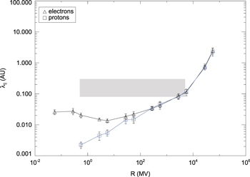
Figure 2. The parallel mean free path vs. magnetic rigidity for pure slab turbulence, the damping model of dynamical turbulence, and δB/B0 = 1.0. The shaded band represents the Palmer (1982) consensus range. The parallel mean free path is shown in astronomical units (AU) and the rigidity is shown in megavolts (MV).
Download figure:
Standard image High-resolution imageFor perpendicular transport we observed subdiffusive transport after the initial ballistic regime. The Unified Nonlinear Transport (UNLT) theory developed in Shalchi (2010) can be used to compute the perpendicular diffusion coefficient analytically for dynamical turbulence (see Shalchi 2014). The latter theory predicts that in the limit  perpendicular diffusion is recovered but the corresponding perpendicular mean free path is very small. The findings of the current paper agree with such analytical predictions in the sense that all our numerical results are larger than the analytical values.
4.2. Slab/2D Turbulence with δB/B0 = 1.0
Since theoretical results obtained by using either quasilinear calculations (see Bieber et al. 1994) or numerical simulations (see previous paragraph) do not agree with observations as long as the slab model is used, we now employ the 20%/80% composite model proposed by Bieber et al. (1994, 1996).
The parallel mean free path versus magnetic rigidity is shown in Figure 3. Although the parallel mean free path is now increased compared to the pure slab result, we are still far below the Palmer consensus range. Whereas quasilinear estimates provide a parallel mean free path that is a factor of five larger compared to the slab result, this effect is much smaller if simulations are used. The physical explanation for that different behavior was presented in Shalchi et al. (2006). For the two-component model used here, resonance broadening due to perpendicular diffusion becomes important. This type of nonlinear effect makes the parallel mean free path smaller compared to the quasilinear result. Thus, we conclude that the idea of replacing the slab model with a two-component model helps to increase the parallel diffusion coefficient, but this effect is not strong enough to achieve agreement with solar wind observations.

Figure 3. The parallel mean free path vs. magnetic rigidity for two-component turbulence, the damping model of dynamical turbulence, and δB/B0 = 1.0. The shaded band represents the Palmer (1982) consensus range.
Download figure:
Standard image High-resolution imageFor the perpendicular diffusion coefficient we found diffusive behavior for all considered cases. The perpendicular mean free path versus magnetic rigidity is visualized in Figure 4 and the ratio of the two diffusion parameters  versus rigidity is shown in Figure 5. The latter ratio is almost constant for small rigidities and then decreases rapidly if the rigidity is increased. According to Figure 4 the perpendicular mean free path eventually becomes constant in the high rigidity limit. This behavior of the perpendicular diffusion coefficient is exactly what is predicted by the UNLT theory, as shown in detail in Shalchi (2015).

Figure 4. The perpendicular mean free path vs. magnetic rigidity for two-component turbulence, the damping model of dynamical turbulence, and δB/B0 = 1.0. For comparison we show observations of Jovian electrons (Chenette et al. 1977, star), Ulysses measurements of Galactic protons (Burger et al. 2000, dots), and the Palmer (1982) value (horizontal line).
Download figure:
Standard image High-resolution image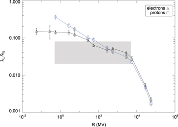
Figure 5. The ratio of perpendicular and parallel mean free paths vs. magnetic rigidity for two-component turbulence, the damping model of dynamical turbulence, and δB/B0 = 1.0. The shaded band represents the Palmer (1982) consensus range.
Download figure:
Standard image High-resolution image4.3. Slab/2D Turbulence with δB/B0 = 0.5
As argued in the previous section, the parallel mean free paths obtained from our simulations are still too small compared to the observations. Those results, however, were obtained for a magnetic field ratio of δB/B0 = 1.0. Ruffolo et al. (2012) suggested that the latter ratio is δB/B0 = 0.5. Furthermore, Tautz & Shalchi (2013) successfully used this magnetic field ratio in their simulations of propagating plasma waves. Thus, we employ the same value here and compute parallel and perpendicular diffusion parameters again.
The parallel mean free path versus magnetic rigidity is shown in Figure 6. We can now clearly see that the electron parallel mean free path goes through the Palmer consensus range. Thus we conclude that we can indeed reproduce the solar wind observations by using our test-particle code. However, besides using the two-component turbulence model, we also have to reduce the magnetic field ratio to δB/B0 = 0.5.

Figure 6. The parallel mean free path vs. magnetic rigidity for two-component turbulence, the damping model of dynamical turbulence, and δB/B0 = 0.5. The shaded band represents the Palmer (1982) consensus range.
Download figure:
Standard image High-resolution imageThe perpendicular mean free path and the ratio of the two diffusion coefficients are shown in Figures 7 and 8, respectively. Qualitatively, the perpendicular diffusion coefficient obeys the same behavior as above, only the magnitudes are different. We compare our numerical findings with observations of Jovian electrons (Chenette et al. 1977), Ulysses measurements of Galactic protons (Burger et al. 2000), and the Palmer (1982) value. Good agreement between the simulations and observations is found.
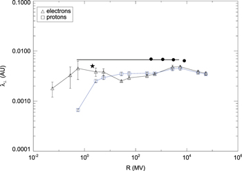
Figure 7. The perpendicular mean free path vs. magnetic rigidity for two-component turbulence, the damping model of dynamical turbulence, and δB/B0 = 0.5. For comparison we show observations of Jovian electrons (Chenette et al. 1977, star), Ulysses measurements of Galactic protons (Burger et al. 2000, dots), and the Palmer (1982) value (horizontal line).
Download figure:
Standard image High-resolution image
Figure 8. The ratio of perpendicular and parallel mean free paths vs. magnetic rigidity for two-component turbulence, the damping model of dynamical turbulence, and δB/B0 = 0.5. The shaded band represents the Palmer (1982) consensus range.
Download figure:
Standard image High-resolution image5. RESULTS FOR THE RANDOM SWEEPING MODEL
In the current paragraph we replace the damping model of dynamical turbulence used above with a random sweeping model where the dynamical correlation function is a Gaussian function (see Table 1). Motivated by the results obtained in Section 4, we only run the simulations for two-component turbulence and a magnetic field ratio of δB/B0 = 0.5.
The parallel mean free path versus magnetic rigidity is shown in Figure 9. Again, the electron parallel mean free path goes through the Palmer consensus range and we can reproduce the solar wind observations by using our test-particle code. By comparing Figures 6 and 9, it can be seen that the results are very similar and the differences between the damping model of dynamical turbulence and the random sweeping model are minor.

Figure 9. The parallel mean free path vs. magnetic rigidity for two-component turbulence, the random sweeping model, and δB/B0 = 0.5. The shaded band represents the Palmer (1982) consensus range.
Download figure:
Standard image High-resolution imageThe perpendicular mean free path and the ratio of the two diffusion coefficients are shown in Figures 10 and 11, respectively. By comparing those results with our findings obtained for the damping model of dynamical turbulence (see Figures 7 and 8), we conclude that there is not a strong influence from the chosen dynamical turbulence model.
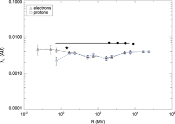
Figure 10. The perpendicular mean free path vs. magnetic rigidity for two-component turbulence, the random sweeping model, and δB/B0 = 0.5. For comparison we show observations of Jovian electrons (Chenette et al. 1977, star), Ulysses measurements of Galactic protons (Burger et al. 2000, dots), and the Palmer (1982) value (horizontal line).
Download figure:
Standard image High-resolution image6. SUMMARY AND CONCLUSION
We have revisited the problem of particle transport in interplanetary space. We have combined test-particle simulations with the model for solar wind turbulence proposed by Bieber et al. (1994). The latter model contains the following key features:
- 1.The spectrum has energy, inertial, and dissipation range and allows us to modify the spectral shape by changing the corresponding indexes q, s, and p;
- 2.The used magnetic correlation tensor contains two contributions or wave modes, namely slab and 2D modes; and
- 3.The turbulence is assumed to be dynamical and we have employed two different models for the dynamical correlations function, namely the damping model of dynamical turbulence and the random sweeping model.
Whereas the used turbulence model is exactly the one described and used in Bieber et al. (1994), our approach to compute particle diffusion parameters is very different. Bieber et al. performed quasilinear calculations, whereas our work is entirely based on computer simulations. Similar simulations have been used before by considering static turbulence (see, e.g., Giacalone & Jokipii 1999; Qin et al. 2002a, 2002b) or undamped propagating plasma waves (see, e.g., Michałek & Ostrowski 1996; Tautz & Shalchi 2013). For the first time we have performed test-particle simulations for dynamical turbulence by employing a more-dimensional Fourier transformation approach, as described in Section 3.
In Figures 2–8 we have shown our numerical findings that were obtained by using the damping model of dynamical turbulence, and compared them with the Palmer (1982) consensus range representing the different solar wind observations. As already concluded by Bieber et al. (1994), we are not able to reproduce the consensus range by simply employing a slab model. The use of a two-component turbulence model is required but even then we are not able to find agreement with the observations. This finding is a major difference between previous work and our simulations. The idea of Bieber et al. (1994) was that by replacing the slab model with a two-component model, we could increase the parallel mean free path drastically. This idea, however, works only in the framework of quasilinear theory. The theory, however, is incorrect due to nonlinear effects, as already pointed out in Shalchi et al. (2004). The simulations are quasi-exact apart from numerical inaccuracies. As shown in the current paper, just replacing the slab model with a slab/2D model alone does not lead to agreement with the observations. Despite the aforementioned issue, we were still able to reproduce the Palmer consensus range by assuming that the turbulent magnetic field is a bit weaker compared to what was assumed before. If we assume that δB/B0 = 0.5, as suggested by Ruffolo et al. (2012), instead of the standard assumption δB/B0 = 1.0, agreement between simulations and observations can indeed be found.
We have repeated our simulations by using the random sweeping model proposed by Bieber et al. (1994). We have again employed the slab/2D model and assumed δB/B0 = 0.5 for the magnetic field ratio. The corresponding results for the parallel mean free path, perpendicular mean free path, and the ratio of the two latter parameters are visualized in Figures 9–11. Our findings are similar to those obtained for the damping model of dynamical turbulence. Again the parallel mean free paths agree very well with the Palmer consensus range.

Figure 11. The ratio of perpendicular and parallel mean free paths vs. magnetic rigidity for two-component turbulence, the random sweeping model, and δB/B0 = 0.5. The shaded band represents the Palmer (1982) consensus range.
Download figure:
Standard image High-resolution image
For the perpendicular diffusion coefficient we found very similar results for the damping model of dynamical turbulence and the random sweeping model. The same applies for the ratio  . We have compared our numerical results with different solar wind observations, namely observations of Jovian electrons (Chenette et al. 1977), Ulysses measurements of Galactic protons (Burger et al. 2000), and the Palmer (1982) value. For two-component turbulence and a magnetic field ratio of δB/B0 = 0.5 good agreement is found for the damping model of dynamical turbulence as well as the random sweeping model.
Reames (1999) argued that the parallel mean free path can be of the order of 1–2 AU for low rigidity particles at a 1 AU heliocentric distance. The largest value for the parallel mean free path in this regime was obtained for the random sweeping model (see Figure 9) where we found  AU. Obviously our numerical results are about a factor of four below the value of Reames (1999). One could try to further reduce the magnetic field ratio δB/B0 or to use a more realistic dynamical turbulence model. This will be subject of future work.
We would also like to point out that there is some similarity between our findings and the results found previously by Tautz & Shalchi (2013). The latter authors, however, used undamped propagating plasma waves, which corresponds to a different turbulence setup. We conclude that propagating plasma waves as well as dynamical turbulence allow for a reproduction of the Palmer consensus range.
We also conclude that the Bieber et al. (1994) turbulence model can indeed be seen as a valid model for particle transport. However, this requires setting δB/B0 = 0.5, a value which is a factor of two smaller compared to the value originally used. Finally, we can state that with this magnetic field ratio we can indeed reproduce solar wind observations by using our test-particle code.
A.S. acknowledges support by the Natural Sciences and Engineering Research Council (NSERC) of Canada. Most simulations shown in this article were obtained by using the national computational facility provided by WestGrid. We are also grateful to S. Safi-Harb for providing her CFI-funded computational facilities for code tests and for some of the simulation runs presented here.