


ABSTRACT
We study the formation of planetesimals in protoplanetary disks from the gravitational collapse of solid over-densities generated via the streaming instability. To carry out these studies, we implement and test a particle-mesh self-gravity module for the Athena code that enables the simulation of aerodynamically coupled systems of gas and collisionless self-gravitating solid particles. Upon employment of our algorithm to planetesimal formation simulations, we find that (when a direct comparison is possible) the Athena simulations yield predicted planetesimal properties that agree well with those found in prior work using different numerical techniques. In particular, the gravitational collapse of streaming-initiated clumps leads to an initial planetesimal mass function that is well-represented by a power law, , with , which equates to a differential size distribution of , with . We find no significant trends with resolution from a convergence study of up to 5123 grid zones and particles. Likewise, the power-law slope appears indifferent to changes in the relative strength of self-gravity and tidal shear, and to the time when (for reasons of numerical economy) self-gravity is turned on, though the strength of these claims is limited by small number statistics. For a typically assumed radial distribution of minimum mass solar nebula solids (assumed here to have dimensionless stopping time ), our results support the hypothesis that bodies on the scale of large asteroids or Kuiper Belt Objects could have formed as the high-mass tail of a primordial planetesimal population.


1. INTRODUCTION
The discovery of thousands of exoplanet systems from Kepler and other missions has confirmed the ubiquity and diversity of planetary systems in our galaxy. The dominant physical processes that lead to the observed configurations of exoplanet systems, however, remain unclear. A central question, for both high- and low-mass planets, is whether what we see reflects the in situ growth of planets from a population of planetesimals, or is instead determined largely by migration at a later stage. Answering this question robustly requires determining, from protoplanetary disk initial conditions, where and when planetesimals form.
In the "bottom-up" model for planet formation, planets are built through several key stages, beginning with the coagulation of small particles into larger particles and particle aggregates, the formation of planetesimals from these solids, and the growth of planetesimals from accretion into larger bodies that become terrestrial planets and the cores of gas giants. In the first step, the collisions of particles through Brownian and turbulent motions lead to their growth into larger bodies. This process is efficient at producing approximately millimeter-size solids (e.g., Brauer et al. 2008; Birnstiel et al. 2010; Zsom et al. 2010). Recent work has shown that it may be possible for solids to grow to approximately centimeter to meter sizes as they drift through radially varying turbulence (Dra̧żkowska et al. 2013), though interior to the snow line, such growth is difficult and solids likely remain stunted at millimeter sizes (Dra̧żkowska & Dullemond 2014).
The propensity of these solids to grow in size only goes so far, however, and forming larger bodies of kilometer size scales or larger (i.e., planetesimal scales) faces two theoretical difficulties. First, if particles grow to sufficiently large sizes (approximately meter sizes at 1 au), they experience a significant head-wind from the sub-Keplerian rotating gas, which causes them to lose angular momentum and rapidly spiral into the star (Weidenschilling 1977). Several mechanisms have been invoked to counteract this drift. For example, pressure bumps due to zonal flows (Johansen et al. 2009a; Simon & Armitage 2014), ice lines (Kretke & Lin 2007; but see Yang & Menou 2010 and Bitsch et al. 2014), and abrupt transitions in ionization fraction (Dzyurkevich et al. 2010; Dra̧żkowska et al. 2013) may stop or slow this radial drift and may even be required given observations showing the presence of these particles at large disk radii (e.g., Andrews et al. 2012).6 However, even if these particle traps are efficient at slowing radial drift, particles still cannot easily grow beyond millimeter to centimeter sizes. A combination of laboratory experiments (primarily on silicates) and modeling shows that particles within this size range do not easily stick together, and instead fragment or bounce (Blum & Wurm 2008; Brauer et al. 2008; Birnstiel et al. 2010; Zsom et al. 2010). Whether this is also the case for icy particles is less clear (e.g.,Blum & Wurm 2008; Okuzumi et al. 2012; Kataoka et al. 2013; Wada et al. 2013; Krijt et al. 2015; Musiolik et al. 2016).
A promising route toward surpassing these difficulties involves instabilities of aerodynamically coupled systems of gas and solid particles. As the gas removes angular momentum from the particles via a headwind, the particles experience inward radial drift. However, the back-reaction of the particle momentum on the gas causes particle over-densities to experience less gas drag as these over-densities act to boost the gas and reduce their own headwind. Therefore, regions of higher particle density will experience slower radial drift, leading to a pile up of solids at various radii. This mechanism is the essence of what is known as the streaming instability (Youdin & Goodman 2005; Johansen & Youdin 2007; Youdin & Johansen 2007; Bai & Stone 2010a, 2010c).
The streaming instability has been studied analytically in the linear regime (Youdin & Goodman 2005; Youdin & Johansen 2007) and in the nonlinear regime via numerical simulations (e.g., Johansen et al. 2007; Johansen & Youdin 2007; Bai & Stone 2010a). The initial growth of the instability does not involve self-gravity, and in this limit, two and three-dimensional (3D) calculations have been used to quantify the strength of clumping as a function of the physical (Johansen et al. 2009b; Bai & Stone 2010c; Carrera et al. 2015), and numerical parameters, e.g., resolution (Bai & Stone 2010b). In particular, Johansen et al. (2009b) and Bai & Stone (2010c) carried out numerical calculations of the streaming instability without self-gravity and found that the instability generally leads to efficient particle clumping when the dimensionless stopping time (i.e., the stopping time multiplied by the orbital frequency) is and the height-integrated solid-to-gas ratio is super-solar. Furthermore, the instability occurs for a wide range in background gas pressure gradients, but for a given metallicity, it favors smaller gradients (Bai & Stone 2010c).

Three-dimensional calculations that include the mutual gravitational forces between particles have been used to study how planetesimals form (Johansen et al. 2007, 2009b, 2011, 2012, 2015). While many characteristics of planetesimal formation have yet to be fully explored, these studies have generally shown that planetesimals with masses consistent with dwarf planets and planetesimals in the main asteroid belt and Kuiper Belt can form after the streaming instability generates sufficiently strong clumps that self-gravity can take over (e.g., Johansen et al. 2007, 2011, 2012, 2015).
These studies have established the streaming instability as the leading candidate mechanism for the efficient formation of planetesimals. Many critical questions, however, remain open. These include whether the streaming instability—in isolation, or in concert with large-scale structures such as zonal flows (Johansen et al. 2009a)—can form planetesimals in the inner disk, where the dimensionless stopping time of millimeter-sized particles . Furthermore, the dependence of the initial planetesimal mass and size distributions on physical properties, such as τ, the metallicity, and gas-phase turbulence is an open issue. Indeed, characterizing these distributions is of substantial importance to explaining properties of both the main asteroid belt and the Kuiper Belt planetesimal populations. To-date, simulations of the streaming instability in the presence of particle self-gravity (Johansen et al. 2015) have revealed a shallower planetesimal size distribution than what is inferred from main belt and Kuiper Belt observations (Jedicke et al. 2002; Morbidelli et al. 2009; Fraser et al. 2010, 2014). However, an extensive systematic survey of the dependence of this distribution on physical parameters has yet to be carried out.

Purely numerical issues are also of interest. The relative strengths and weakness of different numerical schemes are well-characterized in a variety of situations, including low and high-Mach number turbulence, but much less is known in the more complex situation where we have multiple phases, aerodynamic coupling and self-gravity. All previous simulations of planetesimal formation that have included self-gravity have used high-order finite difference methods (implemented in the Pencil code). Here, we instead combine particle self-gravity with a higher order Godunov hydrodynamic scheme (implemented in the Athena code; Stone et al. 2008) to study planetesimal formation and again address the dependence of planetesimal mass and size distributions on numerical effects.
In this paper, the first of a series, we describe our implementation of particle self-gravity within the Athena code, and present results from a baseline set of 3D simulations. Our primary focus is on independently verifying (and in some cases extending) prior numerical simulations of streaming-initiated planetesimal formation, and hence we start with parameter choices that match those in the existing literature. We specifically address the convergence of the initial planetesimal mass function with numerical resolution, and the effect of varying the strength of self-gravity as compared to tidal shear. We also study whether the results depend on when in the simulation particle self-gravity is turned on, given that it is common (and computationally expedient) to do so at a relatively late time when the non-self-gravitating streaming instability is already strongly nonlinear. There has been some study of the impact of this approximation (Johansen et al. 2011), but a detailed investigation of the effects of pre-gravity conditions on the outcome of planetesimal formation has not yet been performed.
The outline of the paper is as follows. Our methodology is described in detail in Section 2, which includes a description of the numerical algorithm and the implementation of particle self-gravity, two test problems to check this implementation, and a description of our streaming instability calculations. In Section 3, we present our results from each set of calculations, and we discuss these results in Section 4. We wrap up with a summary and conclusions in Section 5.
2. METHOD
In this section, we explain our methodology. We first describe the algorithmic details of Athena in the shearing box approximation with the inclusion of aerodynamic coupling between the gas and the particles and the mutual gravitational attraction between particles solved via a Fast Fourier Transform (FFT) method. We then present tests of our particle self-gravity module, followed by a description of our set up, parameters, and diagnostics for the local, streaming instability simulations that we carry out in this paper.
2.1. Numerical Algorithm
Our simulations use Athena, a second-order accurate Godunov flux-conservative code for solving the equations of hydrodynamics and magnetohydrodynamics. The simulations we have carried out here neglect magnetic fields, and we use the hydrodynamics module of Athena. We use the Athena configuration that includes the dimensionally unsplit corner transport upwind method of Colella (1990) coupled with the third-order in space piecewise parabolic method of Colella & Woodward (1984). We use the HLLC Riemann solver to calculate the numerical fluxes (Toro 1999). A detailed description of the base Athena algorithm and the results of various test problems are given in Gardiner & Stone (2005, 2008), and Stone et al. (2008).
The simulations employ a local shearing box approximation. The shearing box models a co-rotating disk patch whose size is small compared to the radial distance from the central object, R0. This allows the construction of a local Cartesian frame that is defined in terms of the disk's cylindrical co-ordinates via , , and . The local patch co-rotates with an angular velocity Ω corresponding to the orbital frequency at R0, the center of the box; see Hawley et al. (1995).


There are two sets of equations to solve. Comprising the first set are the continuity and momentum equation for the gas dynamics:


where ρ is the mass density, is the momentum density, P is the gas pressure, is the identity matrix, is the (dimensional) stopping time of the particles, and q is the shear parameter, defined as q = −dlnΩ/dlnR. We use , appropriate for a Keplerian disk. For simplicity and numerical convenience, we assume an isothermal equation of state , where is the isothermal sound speed. From left to right, the source terms in Equation (2) correspond to radial tidal forces (gravity and centrifugal), vertical gravity, the Coriolis force, and the feedback from the particle momentum onto the gas. The feedback term consists of the local particle mass density , the difference between the particle velocity and gas velocity, and the stopping time of particles due to gas drag. As we describe below, this feedback term is calculated at the location of every particle and then distributed to the gas grid points.


The second set of equations describes the particle evolution. The equation of motion for particle i is given by

where the prime denotes a frame in which the background shear velocity has been subtracted. This is part of the orbital advection scheme (Masset 2000; Johnson et al. 2008; Stone & Gardiner 2010), which has been implemented for the gas dynamics as well. The term accounts for the inward radial drift of particles resulting from a gas headwind, where η is the fraction of the Keplerian velocity by which the orbital velocity of particles is reduced (see Section 2.3). In real disks, this headwind results from a radial pressure gradient that causes the gas to orbit at sub-Keplerian speeds while the particles continue to orbit at Keplerian velocities. However, such a radial pressure gradient is inconsistent with the radial (shearing) periodic boundary conditions in the shearing box model. Following Bai & Stone (2010b), we circumvent this issue by imposing an inward force on the particles, resulting in the term as described above. As a result, both the particles and gas (azimuthal) velocities are shifted to slightly higher values (by ) than what would be present in a real disk, but the essential physics of differential motion between the gas and particles is accurately captured.


Equation (3) is solved using the algorithms described in Bai & Stone (2010b); in particular, we use the semi-implicit integration method combined with a triangular shaped cloud (TSC) scheme to map the particle momentum feedback to the grid cell centers and inversely to interpolate the gas velocity to the particle locations ().

The force due to the particle self-gravity is denoted by , which is found by first solving Poisson's equation for particle self-gravity,


where is the gravitational potential of the particle self-gravity. The force is then calculated via,


In solving Equation (4), we follow the methodology outlined in Section 2.3 and the appendix of Koyama & Ostriker (2009), which consists of a discrete 3D FFT adapted to handle the shearing-periodic boundaries in x and the vacuum boundaries in z. Solving the Poisson equation with FFT requires periodicity in all three-dimensions. In the azimuthal dimension, this is trivially satisfied. For the radial boundaries, the particle mass density (which is distributed to the gas grid points using the same interpolation method as used to calculate the momentum exchange terms; TSC) is mapped to the nearest time in which the shearing-periodic boundaries are purely periodic. From Hawley et al. (1995), the times at which the radial boundaries are purely periodic are with . For each value of x, the particle density is reconstructed along y via a conservative remap; the density is calculated by differencing numerical "fluxes" along y. These fluxes are calculated via third order reconstruction coupled with the extremum preserving algorithm of Sekora & Colella (2009). Note that this reconstruction is the same method employed to remap the fluid quantities in the radial ghost zones as part of the shearing-periodic boundary conditions (Stone & Gardiner 2010).


In the vertical direction, the solution to Equation (4) is found using the Green's function of the Poisson equation for a horizontal sheet of sinusoidal source mass, as described in detail in the appendix of Koyama & Ostriker (2009). The authors of that work developed this method to calculate the potential of self-gravitating gas, but we have trivially extended this same algorithm to use the particle mass density instead of the gas density.
With these methods in hand, the potential is calculated as follows. The particle mass density is reconstructed along y via the same third-order conservative remap as is used for the boundary conditions, multiplied by appropriate functions of z, as described above (see Equation (A11) of Koyama & Ostriker 2009), and then Fourier transformed via a 3D FFT. The density in Fourier space is then multiplied by the appropriate coefficients and transformed back to real space via another 3D FFT (see Equation (A8) of Koyama & Ostriker 2009). In calculating the 3D FFT's, a domain of size is used; twice the vertical domain size is required for the use of Green's function in solving the potential with vacuum boundaries. Finally, the gravitational potential is mapped back to the original time using the third-order conservative remap that was used on the particle mass density.

The resulting is a cell-centered quantity, and we calculate the forces at the cell center using a central finite difference method over three grid cells in every direction. Thus, the force (Equation (5)) in the x-direction in cell is calculated by


and similarly for the y and z directions. The forces then have to be interpolated back to the location of the particles, and we again use the TSC method. We add the self-gravity force to the particles simultaneously with the drag force.
The boundary conditions are the shearing-periodic boundaries in the radial direction, purely periodic in the azimuthal direction, and a modified outflow condition in the vertical direction in which the gas density is extrapolated via an exponential function into the grid zones (Simon et al. 2011, R. Li et al. 2016, in preparation). This latter boundary condition is not standard in shearing box setups for the streaming instability as the small domain size makes it difficult to prevent substantial outflow in the vertical direction. However, in a forthcoming publication by the authors (R. Li et al. 2016, in preparation), we have experimented with the vertical boundary conditions and find that coupled with a routine to renormalize the total mass in the domain to make it constant in time, the outflow boundaries work reasonably well.
The boundary conditions for the gravitational potential are essentially the same as the hydrodynamic variables; shearing-periodic in x and purely periodic in y. The vertical boundary conditions are open, and the potential is calculated in the ghost zones via a third order extrapolation.
2.2. Particle Self-gravity Tests
In this section, we carry out two tests of our numerical algorithm for particle self-gravity. The first test is the collapse of a uniform density sphere of particles. The second test consists of the self-gravitating, shearing wave of particles described in the Supplementary Material of Johansen et al. (2007).
2.2.1. Spherical Collapse
The collapse of a uniform density sphere under its own gravity has a simple analytic solution with which to compare the numerical solution. The equation of motion for a test particle at radius r(t) starting at the outer edge of the sphere is

where M is the total mass within the sphere and remains constant in time. Parameterizing the time dependence of r(t) via , we assume that , where r0 is the initial radius of the uniform density sphere, and find that


The analytical solutions to the radius and mass density are given by


where α is given by Equation (8).
To test our self-gravity solver against this analytic solution, we initialize a sphere of particles with radius on a cubic domain of resolved by 963 zones. Every zone within the radius of the sphere has one particle per grid cell initially. We turn off gas drag on the particles in order to only test the particle self-gravity module. We use TSC interpolation, and the semi-implicit particle integrator. The boundary conditions are open in all three dimensions, and consequently we use the Green's function approach of Koyama & Ostriker (2009) to solving for the potential with vacuum boundaries; here applied to all three dimensions instead of only the vertical as described above. We arbitrarily set the value of G to 8 × 10⁻³.


The solution to this test problem is shown in Figure 1, which depicts the evolution of and versus time in units of the free fall time where is the initial particle mass density. As the figure shows, the numerical solution matches the analytic solution quite well. The differences between the two curves that show up at late times is a result of the FFT solver becoming less accurate as the particles are concentrated into fewer and fewer grid cells. At such particle densities, the discretization error of the FFT solution starts to dominate, as we discuss more below. Even with these errors, the numerical solution does not deviate too much from the analytic solution. This limitation should be kept in mind when considering the formation of planetesimals. In fact, the natural softening length of our FFT solver is where is the length of a grid cell.7


Figure 1. Numerical solution to the particle sphere test problem compared to the analytic solution. The radius of the sphere is shown in the top panel and the particle mass density is shown on the bottom. In both plots, the black curves are the analytic solution, and the red curves are the numerical solution. We plot both the density at the center of the sphere (solid red line) and averaged over the sphere (dashed red line) in the lower plot. Our algorithm for calculating the radial extent of the sphere finds the first cell inward from the boundary in which the particle mass density jumps above 50% of the density at the sphere's center. Thus, our algorithm tends to integrate to just slightly larger than the boundary of the sphere, making both the average density and the sphere radius slightly different than the analytic solution. Otherwise, the numerical solution agrees quite well with the analytic solution. There is some deviation at late times, at which point we expect the numerical solution to deviate from the analytic due to grid-scale effects.
Download figure:
Standard image High-resolution imageTo further test our gravity module, we have also implemented a direct summation method for calculating the mutual gravitational forces between particles. This method is exact, but scales as , where N is the number of particles. For large numbers of particles the direct summation method becomes prohibitively expensive. However, for small numbers of particles we can use this method to compare the forces calculated by the FFT method with the forces from the direct summation, which will be exact to within machine precision. The comparison also tests the accuracy of our interpolation scheme since the direct sum method does not require any interpolation of the gravitational forces to the particle locations. We calculate the error in the force in the ith direction as


where is the force due to self-gravity on particle n calculated via the FFT method and is the same but calculated with the direct summation method. We run the particle sphere collapse problem at a resolution of 323 (and again, one particle per grid cell within the sphere initially) and find that the errors are typically very small early on (on the order of 10−5 or less). As time progresses, the errors grow; as the particles get more concentrated within a smaller number of grid cells, the truncation level error from the particle self-gravity solver will become more and more dominant. At , the average errors are approximately 1% or less, and near , the average errors are on order of a few percent.


2.2.2. Self-gravitating, Shearing Wave
While the spherical collapse problem tests the core of our Poisson solver, we require a problem to test the implementation of this solver in the shearing box setup. To this end, we employ the linearized self-gravitating, shearing particle wave with gas drag described in detail in Section 1.3.1 of the Supplementary Material of Johansen et al. (2007). Following that work, we linearize the continuity equation, equation of motion, and Poisson's equation for a particle "fluid" of density , velocity , and self-gravity potential where prime represents the linear perturbation on the background. The perturbation is assumed to be of the form . Note that we assume uniformity along the vertical direction. The evolution of the density and velocity perturbations are then governed by the following equations:


![${q}^{\prime }(t,x,y)=\delta q(t){\rm{Exp}}[i({k}_{x}(t)x+{k}_{y}y)]$](https://content.cld.iop.org/journals/0004-637X/822/1/55/revision1/apj523488ieqn53.gif)


where the radial wavenumber kx is time-dependent,

We set , , ky = 1, q = 1.5, and . We solve Equations (12)–(14) using a simple finite difference algorithm to obtain our linear solution to the self-gravitating, shearing wave problem in the linear limit. For the numerical test of our algorithm, we initialize a grid of size at resolution and with one particle per cell initially; the small size/resolution in the vertical direction makes the problem effectively two-dimensional while still testing the full 3D FFT algorithm. In this setup, the boundary conditions are shearing-periodic in x and purely periodic in both y and z. Note that we turn off particle feedback to the gas for this test problem.


The time evolution of the amplitude of the perturbations are shown in Figure 2. The numerical solution agrees very well with the linear solution up to amplitudes of . At this point, the numerical solution approaches the nonlinear regime, and agreement between the linear and numerical solutions is not expected. This test problem, which includes several essential ingredients relevant to the streaming instability calculations in this paper, (i.e., shear, self-gravity, and drag), demonstrates the validity of our self-gravity implementation in the shearing box setup.


Figure 2. Amplitude of the perturbations vs. time (in units of ) in the self-gravitating, shearing wave test. The red lines show the numerical solution, whereas the black lines show the linear solution. The solid lines are the density perturbation, , the dashed lines are the x velocity perturbations, , and the dotted–dashed lines are the y velocity perturbations, . There is excellent agreement between the numerical and linear solutions up to amplitudes of , where the numerical solution begins to go nonlinear.


Download figure:
Standard image High-resolution image2.3. Simulation Setup
All of our streaming instability simulations use a shearing box domain of size = . Here, H is the vertical scale height of the gas, which is initialized with a hydrostatic (Gaussian) vertical profile,


where is the mid-plane gas density. We choose code units so that the standard gas parameters are unity; . Given the limited vertical extent of our domain, the gas density does not vary significantly.


The particles are distributed uniformly in x and y and with a Gaussian profile in z. The scale height of this profile is . While we add random noise to the particle locations to seed the streaming instability, it is worth mentioning that the particles are not initially in an equilibrium state. There is radial motion induced by the radial drift term as described above, and the lack of a pressure gradient to counteract vertical gravity means that the particles will settle toward the disk mid-plane.


Four dimensionless quantities characterize the evolution of the streaming instability and the ability of dense clumps to gravitationally collapse. The streaming instability depends upon the dimensionless stopping time,

which characterizes the aerodynamic interaction between a single particle species and the gas, the metallicity,

which is the ratio of the particle mass surface density to the gas surface density , and a radial pressure gradient parameter that accounts for the sub-Keplerian gas in real disks


This radial pressure gradient produces a headwind on the particles, which has velocity a fraction η of the Keplerian velocity. For all of our runs, , metallicity is moderately super-Solar, Z = 0.02, and .


With the inclusion of self-gravity, an additional parameter is needed to describe the relative importance of self-gravity and tidal shear. We define a parameter ,


which describes the strength of self-gravity in the simulation. Physically, varying is equivalent to changing the gas density (and thus through assuming the same Z, the particle mass density) or the strength of tidal stretching (i.e., changing Ω) or both. Thus, in a real disk, will vary with radius, and in a minimum mass solar nebula model (MMSN; Hayashi 1981), this parameter increases very gradually with radius.


In what follows, we convert code units to physical units using the mass unit and assuming a radius of 3 au in an MMSN. For , this equates to . This physical unit conversion depends on , as we discuss further below.


Our fiducial simulation is a relatively low-resolution run with = gas zones and 2,400,000 particles. For this simulation, we turn on self-gravity at a time and set .


2.4. Parameter Variation
We then explore parameter space by varying one parameter in each simulation subset (demarcated in Table 1 by separate boxes). In the first subset, we vary the numerical resolution and the number of particles. We explore a lower resolution with 300,000 particles, and two higher resolutions: with 19,200,000 particles and with 153,600,000 particles. In the next subset, we vary the value of from 0.02 to 0.1; this was chosen to match the test carried out by Johansen et al. (2012) in which the strength of gravity was varied.


Table 1. Streaming Instability Simulations
| Run | Domain Size | Resolution | τ | Z | Comments | |||
|---|---|---|---|---|---|---|---|---|
| () | ||||||||
| SI64-G0.05 | 300,000 | 0.3 | 0.02 | 0.05 | 400 | ⋯ | ||
| SI128-G0.05 | 2,400,000 | 0.3 | 0.02 | 0.05 | 170 | Fiducial Run | ||
| SI256-G0.05 | 19,200,000 | 0.3 | 0.02 | 0.05 | 150 | ⋯ | ||
| SI512-G0.05 | 153,600,000 | 0.3 | 0.02 | 0.05 | 110 | ⋯ | ||
| SI128-G0.02 | 2,400,000 | 0.3 | 0.02 | 0.02 | 170 | ⋯ | ||
| SI128-G0.02_tm20 | 2,400,000 | 0.3 | 0.02 | 0.02 | 150 | Restarted earlier | ||
| SI128-G0.02_tm10 | 2,400,000 | 0.3 | 0.02 | 0.02 | 160 | Restarted earlier | ||
| SI128-G0.02_tp10 | 2,400,000 | 0.3 | 0.02 | 0.02 | 180 | Restarted later | ||
| SI128-G0.02_tp20 | 2,400,000 | 0.3 | 0.02 | 0.02 | 190 | Restarted later | ||
| SI128-G0.05 | 2,400,000 | 0.3 | 0.02 | 0.05 | 170 | Fiducial Run | ||
| SI128-G0.05_tm20 | 2,400,000 | 0.3 | 0.02 | 0.05 | 150 | Restarted earlier | ||
| SI128-G0.05_tm10 | 2,400,000 | 0.3 | 0.02 | 0.05 | 160 | Restarted earlier | ||
| SI128-G0.05_tp10 | 2,400,000 | 0.3 | 0.02 | 0.05 | 180 | Restarted later | ||
| SI128-G0.05_tp20 | 2,400,000 | 0.3 | 0.02 | 0.05 | 190 | Restarted later | ||
| SI128-G0.1 | 2,400,000 | 0.3 | 0.02 | 0.1 | 170 | ⋯ | ||
| SI128-G0.1_tm20 | 2,400,000 | 0.3 | 0.02 | 0.1 | 150 | Restarted earlier | ||
| SI128-G0.1_tm10 | 2,400,000 | 0.3 | 0.02 | 0.1 | 160 | Restarted earlier | ||
| SI128-G0.1_tp10 | 2,400,000 | 0.3 | 0.02 | 0.1 | 180 | Restarted later | ||
| SI128-G0.1_tp20 | 2,400,000 | 0.3 | 0.02 | 0.1 | 190 | Restarted later | ||
| SI128-G0.05-no_clump | 2,400,000 | 0.3 | 0.02 | 0.05 | 0 | ⋯ | ||
| SI128-G0.05-low_clump | 2,400,000 | 0.3 | 0.02 | 0.05 | 40 | ⋯ | ||
| SI128-G0.05-med_clump | 2,400,000 | 0.3 | 0.02 | 0.05 | 170 | Same as Fiducial Run | ||
| SI128-G0.05-high_clump | 2,400,000 | 0.3 | 0.02 | 0.05 | 240 | ⋯ |


Download table as: ASCIITypeset image
Finally, we determine the effect of the state at which self-gravity is initiated by examining two diagnostics in a simulation identical to the fiducial one, but with no self-gravity. The first is the maximum value of the volume-averaged particle mass density, , and the second is a weighted version of the volume-averaged particle mass density, defined as . In general, these two quantities behave similarly, but while the maximum density has been used more frequently in the literature to track the degree of clumping via the streaming instability, it can be largely affected by a small number of grid cells (or even one cell), and the latter quantity is more representative of the degree of clumping over the entire domain. Using both of these diagnostics in concert, we chose restart times of (the "low clumping" case), (medium clumping; this is the same as the fiducial simulation), and (high clumping). We also run one case with self-gravity turned on from the beginning state .


All of these runs are labelled by the numerical resolution employed, the strength of self-gravity, and any other modifying information. For example, run SI128-G0.05-low_clump has 128 zones per dimension, , and is initiated from a "low clumping" state, as described above. All simulations are shown in Table 1 with the parameters outlined and any additional, relevant comments.

2.5. Diagnostics
There are several diagnostics employed in Section 3 that we now describe. First is the maximum particle mass density, as described above, as a proxy for the degree of clumping during the streaming instability. Another often employed quantity is the particle mass surface density, which is simply the integral of over the vertical extent of the domain.

Most of our diagnostics require that we locate gravitationally bound mass clumps (after self-gravity has been included) and calculate their mass. Following the basic arguments in Johansen et al. (2011), we calculate at a given time and use a peak-finding algorithm to locate local maxima in the surface density above a certain threshold. The mass of any given clump is determined by calculating a circular region surrounding the clump and iteratively increasing the radius of this region until the mass enclosed within it equals the mass of a clump that is bound by self-gravity compared to tidal effects. Mathematically, we seek a radius R such that the tidal term, , and the gravitational acceleration of a test particle at the edge of the clump's Hill sphere, are in balance,


when the mass enclosed within our test circle equals Mp, we set R as the Hill radius and Mp as the clump mass.
There are two limitations to our algorithm. First, it has difficulty determining the masses of clumps when two or more clumps are very close together in the xy plane. This is alleviated somewhat by setting a minimum distance, equivalent to the Hill radius of a 0.1 mass (which, as we will see, is consistent with masses at the higher end of the resulting mass distributions), below which the algorithm counts two clumps as being one. Furthermore, we subtract contributions of neighboring clumps that are beyond this minimum distance but still within each clump's Hill radius. This limitation with overlapping clumps is particularly troublesome at early times when gravitationally bound clumps have yet to fully form, yet there are still peaks in . The error associated with overlapping clumps commonly manifests itself as very sharp peaks or troughs in the time evolution of the clump masses. While this limitation causes issues on short timescales when clumps temporarily interact, it does not affect the clump mass on long timescales. As a first order approach to remove this effect, we apply a simple boxcar smoothing technique to the time evolution of clump masses in all that follows.


The second limitation arises from applying a two-dimensional approach to a fully three-dimensional problem. However, even though clumps exist in three dimensions, the particle layer is vertically thin enough to make the two-dimensional clump finding approach a good approximation. Indeed, the algorithm appears to do a sufficient job at finding clumps that remain gravitationally bound as the simulation progresses and does not find too many false positives. Furthermore, as shown in Section 3, the diagnostics that employ this algorithm return results roughly consistent with Johansen et al. (2012), lending support to the idea that our analysis works reasonably well.
From this clump finding algorithm, we calculate both the time history of the mass of the formed clumps and the mass distribution function for these clumps. Many of the simulations form only small numbers of clumps, so we seek a simple functional form to fit to the mass distribution. Consistent with prior work, a power-law differential mass distribution,

works well. Here, C1 is a constant that for the purposes of this paper is arbitrary. We also consider the cumulative mass distribution,

where C2 is another arbitrary constant. We can easily translate Equation (22) to a size distribution to find where .


Under the assumption that the data is drawn from a power-law distribution, the power-law index p of the differential distribution can be determined directly from the set of measured masses using a maximum likelihood estimator (MLE; Clauset et al. 2009). From Equation (3.1) in Clauset et al. (2009), we estimate the value of the power-law index by


where is the minimum value of the planetesimal mass in our data, and n is the total number of planetesimals. The error is given by their Equation (3.2),


Using the MLE for p avoids any binning step, which can introduce bias into the estimate. To visually represent the differential distribution, however, we make a local estimate of by taking to be half the distance in the mass co-ordinate between a given planetesimal and its nearest neighbors. A least squares linear fit in log–log space to versus Mp gives an alternate measure of p, that is very roughly consistent but generally slightly smaller.


Irrespective of the statistical methods used, two cautions are in order. First, the underlying distribution of planetesimal masses formed in the simulations cannot in reality be a simple power law because there is zero probability of forming a body with a mass greater than the total mass of solids in the domain. If the actual distribution is a truncated power law then our naive fit will over-estimate the value of p. Second, our lower-resolution runs form rather small number of planetesimals, and any method for estimating p in this situation is noisy, possibly biased, and liable to return a non-Gaussian distribution of slope estimates. Simple experiments suggest that only the higher-resolution runs, for which there are on order 100 planetesimals, can be expected to return robust estimates of the distribution.
3. RESULTS
In this section, we present the results from our various parameter studies. We first describe the properties of the fiducial simulation SI128-G0.05 in detail, followed by quantifying the effects of changing the strength of gravity, the numerical resolution, and the degree of clumping when self-gravity is initiated. Each study is described in its own subsection and the simulations corresponding to each study are presented in Table 1.
3.1. Fiducial Run
In this section, we describe some properties of our fiducial run, SI128-G0.05. Self-gravity is switched on at , after which the mutual gravitational attraction between particles causes the particle density to increase; in units of the initial mid-plane gas density, the maximum particle density rapidly increases to , and then slowly increases to afterward.


A time progression of the particle surface density is shown by a series of snapshots in Figure 3. The streaming instability produces several azimuthally extended structures at early times, which eventually form into one large clumping structure. After self-gravity turns on, some of the high density regions collapse and become gravitationally bound structures with a variety of masses. Near the end of the simulation, there are on order 10 of these bound structures, to which we refer from now on as planetesimals.

Figure 3. Four snapshots during the fiducial simulation, SI128-G0.05. Shown is the logarithm of the vertically integrated particle surface density normalized to the average particle surface density. Time increases from top left to bottom right. The bottom left is shortly after self-gravity is turned on, and the bottom right is well after the planetesimals have formed.
Download figure:
Standard image High-resolution imageThe evolution of the mass of these planetesimals is shown in Figure 4; both the total mass and maximum mass are shown. This evolution can be compared to Figure 13 of Johansen et al. (2012). Although, most of the simulations in Johansen et al. (2012) contain collisional microphysics, they find that the mass evolution of planetesimals only depends very weakly on this, if at all. We find that the total and maximum masses in units of the mass of Ceres are approximately the same by in our fiducial simulation and the simulation of Johansen et al. (2012). Our simulations show a faster growth rate for the masses of planetesimals. Given the difficulties associated with the clump finding analysis early on, some differences are not surprising. However, that we find approximately the same values for the maximum and total masses is encouraging.


Figure 4. Evolution of the total mass in planetesimals (solid line) and maximum planetesimal mass (dashed line) over time in our fiducial simulation. The mass is given in units of the mass of Ceres. Time is in units of and is measured from the initialization of self-gravity onward. We find general agreement with a similar run in Johansen et al. (2012), but there are some differences in the initial growth rate of planetesimals.

Download figure:
Standard image High-resolution imageFinally, we analyze the mass and size distribution of these planetesimals. We find that there are 13 clumps, and roughly, the number of these clumps increases toward the low-mass end.
Choosing the point at which to calculate the mass distribution is a bit subtle. Our general approach is to visually inspect the particle mass density (e.g., Figure 3) and choose a time shortly after planetesimals have formed (so as to not sample later times when these planetesimals have substantially grown in mass due to accretion of smaller particles and/or mergers) and have become separate objects (i.e., no significant overlap with the over density of mass from which they formed). We have calculated the mass distribution at three different times; , and . While the large scatter in the differential mass makes a comparison between the different snapshots and a precise quantification of the power-law slope difficult, we find approximate "by-eye" agreement in the values of Mp and . To reduce the noise inherent in the differential mass distributions, we also checked the cumulative distributions at these three times and found excellent agreement. Thus, we are confident that there is not a substantial variation in the clump properties over short timescales.


The significant scatter present in the mass distribution brings into question any robust quantification of the value of p. The best-fit value of p from this simulation is clearly there is a large error on p. In order to improve the statistics, we have run four additional simulations with the same parameters as this fiducial run, but restarted from the "parent" non-self-gravitating simulation at different times. Specifically, we initiated self-gravity at before, before, after, and after the fiducial run. These runs are included in Table 1; the run appended with "tm20" ("tp20") means self-gravity is initiated at the fiducial case restart time minus (plus) . We chose these relatively large time displacements to reduce the likelihood that we would be sampling planetesimals that occur from quite nearly the same initial conditions; in such a case, the formation of planetesimals would not be independent. The result is shown in Figure 5. We fit this data with a power law and now find the error has been reduced by roughly a factor of three.


Figure 5. Differential mass distribution functions for the fiducial simulation along with the four simulations that were restarted at different times to improve statistics. Both the mass and the differential mass function are given in units of Ceres mass. A best-fit power law is over plotted as a dashed line of the corresponding color of the data. The best-fit power-law slope is .

Download figure:
Standard image High-resolution imageThere is a question of whether or not the properties of the distribution of planetesimal masses depend on the time at which self-gravity is activated. We carry out such an investigation below, and as described further in that section, we find that these properties do not appear to have any strong correlation with the initial state, justifying this approach.
3.2. Effect of Resolution
Figure 6 shows a snapshot of the particle mass surface density for each resolution. As with the fiducial simulation, the time chosen in each case is sufficiently long after self-gravity has been turned on for bound planetesimals to form, but sufficiently early so as to avoid the effect of merger events and additional mass accretion onto the formed planetesimals. The times corresponding to these snapshots are also chosen in the calculation of the mass distribution function below. As expected, the size of the largest planetesimals decrease as the grid scale decreases; the minimum radius follows the grid zone size. Furthermore, as resolution is increased, the number of planetesimals increases and the smallest bound mass decreases. From resolution 643 to 5123, the number of formed planetesimals at this time are 2, 13, 30, and 53, respectively.

Figure 6. Snapshot of planetesimal formation at each of the four different resolutions. Shown is the logarithm of the vertically integrated particle surface density normalized to the average particle surface density for runs SI64-G0.05 at (top left), SI128-G0.05 at (top right), SI256-G0.05 at (bottom left), and SI512-G0.05 at (bottom right). Each planetesimal is marked via a circle of the size of the Hill sphere. In some cases of extreme overlap between planetesimals, only one circle is drawn. As resolution is increased, more planetesimals are produced, and the number of smaller planetesimals increase.


Download figure:
Standard image High-resolution imageIn order to show the development of these small-scale structures in the highest-resolution run, we have plotted the various stages of the streaming instability before and after self-gravity was turned on in Figure 7. As both Figures 6 and 7 show, there is significant structure present on small scales, though the large-scale structure remains consistent with the lower-resolution runs. In particular, there are large-scale axisymmetric enhancements in the particle mass density. Once self-gravity has been activated, the smaller structure available at the higher resolution allows smaller-mass planetesimals to condense out of the high densities induced by the streaming instability. Despite the increase in the number of planetesimals at small scales, larger-mass planetesimals still form.

Figure 7. Three snapshots during the highest-resolution simulation, SI512-G0.05. Shown is the logarithm of the vertically integrated particle surface density normalized to the average particle surface density. Time increases from left to right. The left panel shows the clumping due to the streaming instability in the absence of self-gravity but right before self-gravity is activated (). The middle panel corresponds to a point shortly after self-gravity was activated (), and the right panel corresponds to a time in which most of the planetesimals have formed (). In the middle and right panel, each planetesimal is marked via a circle of the size of the Hill sphere. Planetesimals continue to form and to grow in mass during the simulation, as demonstrated by the larger number and increased size of Hill spheres in the right panel. In some cases of extreme overlap between planetesimals, only one circle is drawn. Compared with the lower-resolution simulation, smaller scale structure and the development of more numerous and smaller planetesimals is observed in the particle density.


Download figure:
Standard image High-resolution imageThis resolution effect is also demonstrated via the differential mass distribution, shown in Figure 8. We do not include a power-law fit to either the SI64-G0.05 planetesimals since there are only two objects formed at that resolution or to the SI128-G0.05 planetesimals because we only include the single standard run here (in order to more clearly see the effect of the resolution on the number of planetesimals). Furthermore, the time chosen for the highest-resolution run was taken to be the end of the simulation. It is not entirely clear if planetesimals have stopped forming by this point, and the very high computational expense of this simulation makes integrating further not feasible at this time.

Figure 8. Left: differential mass distribution for SI64-G0.05 at (red triangles), SI128-G0.05 at (black asterisks), SI256-G0.05 at (blue crosses), and SI512-G0.05 at (purple diamonds). Both the mass and the differential mass function are given in units of Ceres mass. We only include the points from the single fiducial 1283 run in order to properly show the effect of resolution on the total number of planetesimals. For the two highest-resolution simulations, a best-fit power law is over plotted as a dashed line of the corresponding color of the data. Right: power-law index, p vs. resolution in number of grid zones along any given dimension with one sigma uncertainties to the fit represented by error bars. The value of p for 1283 here does include the additional four simulations as described in Section 3.1. The power-law slope is for SI128-G0.05, for SI256-G0.05, and for SI512-G0.05. With the exception of the lowest resolution, the mass at the high end of the mass distribution is roughly constant with resolution. As resolution is increased, there are more low-mass planetesimals. There is no consistent trend of the slope with resolution.


Download figure:
Standard image High-resolution imageWith the exception of the lowest resolution, the highest mass planetesimals are for all resolutions. The higher masses (by only a factor of a few) in the 643 run could be related to more rapid growth of the planetesimals that do form since their physical cross section will be larger. However, since there are only two planetesimals, very small number statistics make this notion difficult to test.

The power-law slope is for SI128-G0.05, for SI256-G0.05, and for SI512-G0.05. There is substantial scatter around the best-fit power-law functions, as the figure shows, though the number of formed planetesimals increases with higher resolution, improving the statistics somewhat. In the right panel of Figure 8, we plot the power-law index p with the errors given by Equation (25). There does not appear to be any significant trend in the value of p with resolution, and –1.8.


Our best-fit value of p for the highest-resolution simulation is the same as that found for the 5123 simulation of Johansen et al. (2015); they found a value of p = 1.6 by fitting the cumulative distribution to a power law with an exponential tail. Furthermore, comparing the left panel of Figure 8 to Figure 3 of Johansen et al. (2015) reveals similar scatter about the best-fit line for each resolution.
3.3. Strength of Gravity
We vary to match a similar exploration of this parameter in Johansen et al. (2012); specifically, . Note that with the exception of one of the simulations with , the Johansen et al. (2012) simulations included collision microphysics. However, as discussed above, these authors concluded that the collisions did not have a strong impact on the formation of planetesimals, making a comparison between our work and theirs viable.


Figure 9 shows the mass evolution of the planetesimals for the three values of . Both the total and maximum planetesimal mass increase with increasing gravity. This figure can be compared to Figure 13 of Johansen et al. (2012). In general, we find good agreement with their results; the mass values differ by a factor of less than two. Furthermore, there is no systematic direction in which the masses differ; i.e., some of the mass values in Johansen et al. (2012) are larger than what we find for the same , and others are smaller. Given the differences likely present in the clump finding algorithms, we believe that the agreement is pretty strong.


Figure 9. Total (left) and maximum (right) mass in planetesimals as a function of time for = 0.02 (dashed, green line), 0.05 (solid, black line), and 0.1 (dotted–dashed, orange line). The mass is given in units of the mass of Ceres, and time is in units of and is measured from the initialization of self-gravity onward. On the plot, we denote the dimensionless gravity parameter with G instead of . The total and maximum planetesimal masses increase with increasing . We find general agreement with Figure 13 of Johansen et al. (2012), but there are some differences in the initial growth rate of planetesimals.


Download figure:
Standard image High-resolution imageIn converting the planetesimal mass to physical mass units (to normalize by ), the gravity parameter is folded into the calculation. Thus, a more meaningful comparison between these simulations is to renormalize the planetesimal mass to the total mass in the grid, which is independent of . This is shown in Figure 10. While the total and maximum planetesimal masses increase with as was the case in Figure 9, the differences between the curves are significantly reduced, and the maximum mass of SI128-G0.02 and SI128-G0.05 appear to be roughly the same.


Figure 10. Same as Figure 9 but with the planetesimal mass normalized to the total particle mass in the domain. The renormalization of mass reduces the difference between the different values. However, the total and maximum planetesimal masses still increase with increasing .


Download figure:
Standard image High-resolution imageAs with the previous simulations, we calculate the differential mass distribution. The result is shown in Figure 11. As with the fiducial calculation, we have run an additional four simulations for each value of corresponding to self-gravity activated at and both before and after the time that it is activated in the reference simulations. As before, this approach significantly improves the statistical scatter in the mass distribution plot.


Figure 11. Left: differential mass distribution at for (green diamonds), for (black asterisks), and for (orange triangles). Both the mass and the differential mass function are given in units of Ceres mass. On the plot, we denote the dimensionless gravity parameter with G instead of . In each case, a best-fit power law is over plotted as a dashed line of the corresponding color of the data. For each value of , we include the four simulations that were restarted at different times to improve statistics. Compared to the and runs, a later time relative to the activation of particle self-gravity is chosen to analyze the simulations because the planetesimals take a longer time to become separate, bound clumps. Right: the best-fit power-law index p as a function of . The best-fit slope is for , for , and for . The mass distribution shifts toward larger masses with increasing . There is no consistent trend in the value of p with .


Download figure:
Standard image High-resolution imageWe examine the best-fit power-law slope as a function of in the right panel of Figure 11. The power-law slope is for , for , and for there is some variance in p with , but these values fall within the range of p = 1.4–1.8.


Despite the improvement introduced by combining simulation data, there is still significant scatter in the values of the differential mass function. To remove some of this noise, we calculate the cumulative mass distribution for each value of as shown in Figure 12. As with the differential mass distribution, the slope of the distribution remains roughly constant with , but the distribution shifts toward larger mass.


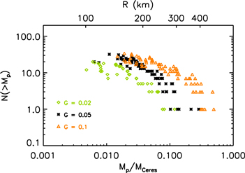
Figure 12. Cumulative mass distribution for (green diamonds), (black asterisks), and (orange triangles). On the plot, we denote the dimensionless gravity parameter with G instead of . For each value of , we include the four simulations that were restarted at different times. The mass distribution shifts toward larger masses.


Download figure:
Standard image High-resolution image3.4. Effect of Initial Clumping
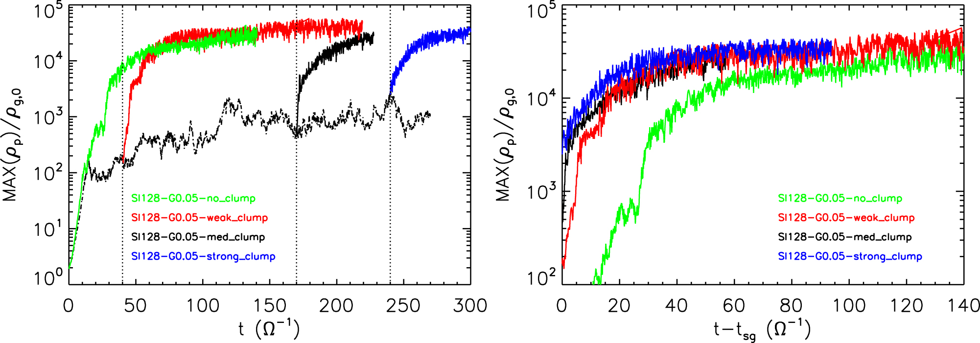
In this section, we consider the effect of changing the time at which particle self-gravity is activated. We first consider the maximum particle mass density as a function of time for this series of simulations, which is shown in Figure 13. There is a clear difference in the initial growth of depending on the initial degree of clumping from which the simulation was activated. At late times, the maximum particle density reaches approximately the same level for all four simulations.


Figure 13. Maximum of the particle mass density, normalized to the initial mid-plane gas density, as a function of time for simulations in which self-gravity was initiated at different degrees of clumping via the streaming instability. The green line corresponds to the "no clumping" case, SI128-G0.05-no_clump, red is the "weak clumping" case, SI128-G0.05-weak_clump, black is the "medium clumping" case, SI128-G0.05-med_clump, and blue is the "strong clumping" case, SI128-G0.05-strong_clump. The left plot includes the non-self-gravitating run (dotted–dashed line) from which these various simulations were restarted, whereas the right panel displaces the temporal axis by the restart time so that the various density evolutions can be more directly compared. The growth rate of maximum particle density decreases with decreasing degree of clumping, though at late times, the maximum particle density is approximately the same between all runs.
Download figure:
Standard image High-resolution imageThese basic results are corroborated by examination of the total and maximum planetesimal mass evolution, as shown in Figure 14. We should reiterate that the initial stages of growth should be treated with some caution here due to the possible presence of false-positives and overlapping clumps that cause errors in our clump-finding algorithm. However, that the initial evolution is generally consistent with the evolution of the maximum particle density in Figure 13 is encouraging.

Figure 14. The total (left) and maximum (right) planetesimal mass as a function of time for simulations in which self-gravity was initiated at different degrees of clumping via the streaming instability. The green line corresponds to the "no clumping" case, SI128-G0.05-no_clump, red is the "weak clumping" case, SI128-G0.05-weak_clump, black is the "medium clumping" case, SI128-G0.05-med_clump, and blue is the "strong clumping" case, SI128-G0.05-strong_clump. The growth rate of planetesimal masses decreases with decreasing degree of clumping. At late times, the masses of the four simulations become roughly equal.
Download figure:
Standard image High-resolution imageGiven the different growth rates for the planetesimals in each of these runs, one has to be careful in choosing the correct times to analyze properties of the planetesimal distribution. Our general method has been the same as described above; visually examine the collapse of planetesimals and then average the mass distribution over a period corresponding to roughly when individual clumps can be identified but before there is significant merging between these clumps.
As shown in Figure 14, there is a steep growth early on in SI128-SG-weak_clump, followed by a relatively flat evolution, which is then followed by growth again. This second growth period, which happens roughly between and , is due to a second phase of planetesimal formation. From an examination of the particle surface density evolution, this second phase of planetesimal formation appears to follow the formation of another largely axisymmetric enhancement in the particle density. Apparently, in this particular simulation, the conditions allowed the streaming instability to act on remaining small solids in the disk after the initial formation of planetesimals. The second density enhancement induced by the streaming instability then went gravitationally unstable and added to the total number of planetesimals.


In choosing our analysis time for SI128-G0.05-weak_clump, we thus chose a time after the second period of planetesimal growth. At the chosen times, SI128-G0.05-no_clump produces 11 clumps, SI128-G0.05-weak_clump produces 10, SI128-G0.05-med_clump produces 13, and SI128-G0.05-strong_clump produces 11.
In Figure 15, we plot the differential mass distribution for the four different start times. There is significant scatter in the differential mass function, but the power-law indices appear roughly consistent between the different simulations. Specifically, for SI128-G0.05-no_clump, for SI128-G0.05-weak_clump, for SI128-G0.05-med_clump, and for SI128-G0.05-strong_clump. These p values are slightly larger than that found for the previously discussed simulations, which is a result of smaller number statistics biasing the fitted slope value, as we found for the fiducial run in Section 3.1.


Figure 15. Left: differential mass distribution for simulations with self-gravity activated at different times. The green line corresponds to the "no clumping" case, SI128-G0.05-no_clump, red is the "weak clumping" case, SI128-G0.05-weak_clump, black is the "medium clumping" case, SI128-G0.05-med_clump, and blue is the "strong clumping" case, SI128-G0.05-strong_clump. Both the mass and the differential mass function are given in units of Ceres mass. In each case, a best-fit power law is over plotted as a dashed line of the corresponding color of the data. Right: the best-fit power-law index p as a function of activation time. The best-fit values are for SI128-G0.05-no_clump, for SI128-G0.05-weak_clump, for SI128-G0.05-med_clump, and for SI128-G0.05-strong_clump.


Download figure:
Standard image High-resolution imageAs we did in Section 3.3, we calculate the cumulative mass distribution to reduce the noise inherent in the differential distribution. This is shown in Figure 16.

Figure 16. Cumulative mass distribution for simulations initiated with self-gravity activated at different times The green triangles correspond to the "no clumping" case, SI128-G0.05-no_clump, red squares are the "weak clumping" case, SI128-G0.05-weak_clump, black asterisks are the "medium clumping" case, SI128-G0.05-med_clump, and blue diamonds are the "strong clumping" case, SI128-G0.05-strong_clump.
Download figure:
Standard image High-resolution imageRoughly speaking, there does not appear to be significant differences between the mass distributions in each of these simulations. They all occupy roughly the same space in the differential distribution plot. Based on all of these results combined, it seems that the properties of the planetesimals do not strongly depend on the initial state from which they collapse.
4. DISCUSSION
The initial size distribution of planetesimals has a number of astrophysical implications. Planetesimals that are too small may be subject to turbulent stirring and collisional destruction (Ormel & Okuzumi 2013), while planetesimals that are too large will accrete less efficiently on to giant planet core as a consequence of less efficient gravitational focusing. While important, independent uncertainties in the modeling of these processes make it hard to use them for quantitative constraints on planetesimal size. The best prospect for a direct comparison between theory and observations thus remains studies of the size distribution of small bodies in the Solar System. From our simulations we predict that p generally lies in the range 1.4–1.8, which equates to a slope of the differential size distribution q = 2.2–3.4. For reasonable choices of parameters, we find that the largest bodies in the region of the asteroid belt have masses , corresponding to a size of several hundred km.

The two largest populations of small bodies in the Solar System with which to compare our results are the main asteroid belt and the Kuiper Belt. The asteroid belt has experienced substantial dynamical depletion (which does not alter the sizes of surviving bodies) and collisional evolution in the time since it formed, and detailed modeling is needed to assess whether the current size distribution preserves information about the primordial population. Using such modeling, Morbidelli et al. (2009) have argued that reproducing the current size distribution of asteroids requires primordial planetesimals with diameters , and that the slope of the current size distribution above roughly this scale is similar to the initial slope. To the extent that our work agrees with prior simulations in predicting the prompt formation of some very massive planetesimals, the Morbidelli et al. (2009) analysis supports the scenario of streaming-initiated planetesimal formation. However, the power-law index for the size distribution of asteroids larger than 120 km in diameter (which is relevant to our calculations) is (Jedicke et al. 2002; Bottke et al. 2005). This would correspond to , which is significantly steeper than the power-law portion of the predicted mass function. We note, however, that if the most massive planetesimals are identified with the most massive (surviving) asteroids, then the observed slope would correspond to the region near the cut-off in the primordial mass function, and would be expected to be steeper than the power-law fit seen at lower masses.


Similar arguments apply to the Kuiper Belt. Fraser et al. (2010) calculated the observed luminosity function of the Kuiper Belt and found a value of for the cold classical Kuiper Belt objects and q = 2.8 for the excited, hot Kuiper Belt population. Later corrections to this work (Fraser et al. 2014) that removed the model dependence associated with uncertainties in the distance to KBOs found even steeper values of q = 8.5 (cold population) and q = 5.4 (hot population). Moreover, the largest Kuiper Belt objects are bigger than those in the main asteroid belt. This is consistent with a streaming instability model, since a robust inference from our simulations with varying is that for larger gravity parameters, more massive planetesimals tend to form. In a MMSN (Hayashi 1981), slowly increases with radius (at the location of the asteroid belt, , and at 40 au, ), suggesting that larger planetesimals should be formed at further distances from the Sun. However, as with the asteroid belt, the observed slopes are not what we predict for the primordial population.


The above comparisons are suggestive but should be regarded as preliminary. In addition to the uncertainties in deciphering what the current size distributions in the asteroid and Kuiper belts tell us about the primordial population, there are several sources of possible uncertainty in the prediction of the size distribution itself. First, at a purely numerical level, the collapse of planetesimals in our simulations is halted at the grid scale, which is unphysically large. The cross-section for subsequent accretion or mergers is therefore boosted, which could impact the measured size distribution. We note, however, that the recent simulations of Johansen et al. (2015)—in which collapsed planetesimals were replaced with sink particles—yielded roughly consistent values of p and q as compared to our 5123 simulation. Thus, it would seem that there are no systematic errors in the determination of p with high-resolution simulations.
The largest scales in the box may also play an important role in properties of collapsed planetesimals. Indeed, it has been recently shown through non-self-gravitating simulations that the domain size influences the temporal and spatial properties of particle clumping during the nonlinear state of the streaming instability (Yang & Johansen 2014). It is entirely conceivable that such effects will influence the outcome of the gravitational collapse phase, and we are currently pursuing such investigations (Li et al. 2016, in preparation).
Numerical effects aside, however, it is possible that the size distribution of planetesimals formed from gravitational collapse is not universal, and may be different in the physical environment relevant to the asteroid or Kuiper belts. The streaming instability can produce strong clumping of solids across a wide region in the parameter space of metallicity, radial gas pressure gradient and particle size (Bai & Stone 2010c; Carrera et al. 2015). These parameters are expected to vary substantially with disk radius (for example, the dimensionless stopping time for particles in the asteroid belt region is likely to be much smaller than for the Kuiper Belt region), and this may result in different size distributions after gravitational collapse.
It is also conceivable that the size distribution is a function of how unstable the disk is to the streaming instability and gravitational collapse. We have simulated a system in which a significant fraction of the total mass of solids forms planetesimals on a timescale of just . Meteoritic evidence from the asteroid belt, conversely, suggests a broad spread in the formation times of primitive material (Villeneuve et al. 2009). This can be interpreted as implying that planetesimal precursors persist in the disk over timescales more akin to . It is not known whether a marginally unstable system would form the same planetesimal mass function as the one that we have simulated.


Furthermore, it is worth noting that the size distribution at the end of the gravitational collapse can be subsequently modified by the longer term accretion of planetesimals and smaller solids. The effects of this accretion depend on the evolving size distribution of solids and the evolution of the gas, including its turbulent state (e.g., Johansen et al. 2015). However, the size distribution at the end of the collapse phase, as studied here, is important as input for these longer term accretion studies.
5. CONCLUSIONS
We have developed and tested a module for the mutual gravitational interaction of particles in the Athena code and applied it to preliminary studies of the streaming instability under the influence of particle gravity. As this is the first study of planetesimal formation with the Athena code, we have carried out a basic parameter sweep in order to provide a baseline of calculations and results from which to spawn further investigations and with which to compare the results already present in the literature.
In this paper, we have varied the numerical resolution, the relative strength of gravity and tidal effects, and the degree of clumping induced by the streaming instability before the activation of particle self-gravity. While we will follow up this study in future papers to explore more parameters, we can draw some preliminary conclusions from this work.
- 1.The streaming instability leads to enhanced particle clumping, after which the mutual gravitational attraction between solid particles leads to the formation of a number of bound planetesimals.
- 2.For the choice of metallicity and stopping time used here, the masses of these planetesimals range from to . The typical radii of these planetesimals are 50 km to a few hundred km.
- 3.Where a direct comparison is possible, we find excellent agreement between planetesimal properties in our Athena simulations and those carried out with the Pencil code.
- 4.As resolution is increased, more planetesimals are produced at lower masses and smaller radii, while the high-end mass of the distribution remains approximately the same. There is no significant trend of the power-law index p with resolution. The values of p fall within the range –1.7.
- 5.The power-law slope of the size distribution for the highest-resolution simulation is q = 2.8, which is significantly shallower than that measured for both the main asteroid belt () and the classical Kuiper Belt (cold population; hot population; ).
- 6.Varying the relative strength of gravity through the parameter changes the mass range of planetesimals produced. The value of p does not appear to have any consistent trend with .
- 7.The properties of planetesimals appear largely independent of the initial degree of clumping before gravity takes over, justifying the method employed here and in various papers by Johansen and co-authors of activating particle self-gravity after the streaming instability has already produced clumps.


As this is an initial step into planetesimal studies with Athena, we have only explored a few parameters. A more complete study of planetesimal properties will require varying other parameters, both physical (e.g., metallicity, particle size, radial pressure gradient) and numerical (e.g., boundary conditions and domain size). We will address these issues in future publications.
A more serious uncertainty lies in the relatively small mass and size range produced by the moderate resolution 1283 simulations, which generally spans only a decade in mass. While we were able to alleviate the resulting issue of small number statistics associated with this limited mass range by combining data sets the small mass end of the distribution is ultimately determined by the finite grid scale. Going to higher resolution and a larger number of particles is the obvious solution to this problem, and indeed the highest-resolution 5123 simulation spanned nearly two mass decades. However, such a simulation is very computationally expensive and this expense makes a large exploration of parameter space infeasible.
In a similar vein, at any given resolution, we do not resolve compact planetesimals; i.e., the planetesimals that do form are large compared to the size of planetesimals that would form if we resolved particle self-gravity below the grid scale. These unphysical sizes can cause enhanced accretion of smaller solids onto formed planetesimals and make the power-law distributions shallower. The future implementation of sink particles or sub-grid-cell gravity will help to alleviate these issues.
Despite these uncertainties, our first principles calculations provide additional evidence that the streaming instability can form planetesimals with properties consistent with Solar System constraints. The largest remaining source of uncertainty may be in the initial metallicity and particle size distribution (i.e., prior to the onset of the streaming instabilty). If the appropriate initial conditions can be pinned down via astronomical observations, more comprehensive numerical simulations should be able to provide a detailed understanding of the formation and evolution of the planetesimal population.
We thank Daniel R. Wik for his handy knowledge of statistics and Katherine Kretke for many discussions on observational constraints of Solar System planetesimal populations. We also thank Hal Levison, Anders Johansen, Xue-Ning Bai, and Chao-Chin Yang for useful discussions regarding this work and the referee, whose suggestions greatly improved the quality of this work. We acknowledge support from NASA through grants NNX13AI58G and NNX16AB42G (P.J.A.), from the NSF through grant AST 1313021 (P.J.A.), and from grant HST-AR-12814 (P.J.A.) awarded by the Space Telescope Science Institute, which is operated by the Association of Universities for Research in Astronomy, Inc., for NASA, under contact NAS 5-26555. J.B.S.'s support was provided in part under contract with the California Institute of Technology (Caltech) and the Jet Propulsion Laboratory (JPL) funded by NASA through the Sagan Fellowship Program executed by the NASA Exoplanet Science Institute. The computations were performed on Stampede and Maverick at the Texas Advanced Computing Center through XSEDE grant TG-AST120062.
Footnotes
- 6
Although, as shown by Birnstiel et al. (2012), the presence of small grains at large radii may be the result of the very long timescales over which these grains are swept up by larger solids.
- 7
The grid cell is uniform along all three dimensions; .
