


ABSTRACT
Solar wind fluctuations admit well-documented anisotropies of the variance matrix, or polarization, related to the mean magnetic field direction. Typically, one finds a ratio of perpendicular variance to parallel variance of the order of 9:1 for the magnetic field. Here we study the question of whether a kinetic plasma spontaneously generates and sustains parallel variances when initiated with only perpendicular variance. We find that parallel variance grows and saturates at about 5% of the perpendicular variance in a few nonlinear times irrespective of the Reynolds number. For sufficiently large systems (Reynolds numbers) the variance approaches values consistent with the solar wind observations.
Export citation and abstract BibTeX RIS
1. INTRODUCTION
Plasma turbulence in the presence of a mean magnetic field,  , shows several types of anisotropy, including correlation anisotropy, which is related to the spectrum; temperature anisotropy, which is related to kinetic effects; and variance anisotropy, which is related to the variance matrix of a vector field such as the fluctuation magnetic field
  or plasma fluid velocity
  . In the present paper we focus on the latter type of anisotropy, which can be quantified in terms of the diagonal elements of the variance tensor
  and is sometimes called "polarization" anisotropy (Coleman 1968; Belcher & Davis 1971; Barnes 1979). Here, the angle brackets denote an appropriate average and the variance matrix is written for the particular case of the total magnetic field
  , expressed as the sum of its average value and the fluctuation about that.
It is well established that solar wind fluctuations exhibit a distinctive variance anisotropy with parallel variance usually much less than perpendicular variance. The typical "5:4:1" ratios of component variances  , where the mean field is along z (e.g., Belcher & Davis 1971), are widely believed to correspond to the relative absence of parallel variances. The latter are a general feature of both incompressible and compressible plasma dynamics, including fluid limits. Despite this, their presence is often taken as being indicative of compressive activity and they are frequently entirely ignored in incompressible MHD models of turbulence like critical balance and "slab + 2D" (e.g., Goldreich & Sridhar 1995; Bieber et al. 1996). For a recent review of spectral and variance anisotropy, see Oughton et al. (2015) who summarize solar wind observational results and simulations of related homogeneous turbulence processes. For the effects of expansion on variance anisotropy, see Völk & Aplers (1973) and Verdini & Grappin (2015).
A familiar justification for the connection between parallel variance and compressible physics lies in the domain of MHD wave physics, wherein the small amplitude incompressive Alfvén mode is fully transverse and, for the unidirectional case, can be extended into the large-amplitude regime by imposing constant magnetic pressure (Barnes 1979). This is in contrast to the magnetosonic modes, which typically have a parallel amplitude component and are of course compressible. In addition, though, even in the case of strong turbulence one can show that the asymptotic approach to incompressibility at plasma beta order one (or small) requires that the parallel variance be greatly suppressed (Zank & Matthaeus 1993). In the computational arena, it is also established that beginning with fully isotropic fluctuations, compressible MHD leads to suppressed parallel variance, but incompressible MHD does not (Matthaeus et al. 1996).
Clearly, however, the above understanding is not a complete treatment of the underlying physics, as one would like to know, for example, whether a strongly turbulent system consisting entirely of fully transverse "Alfvénic mode" fluctuations remains in such a state. We emphasize that such fluctuations do not necessarily represent shear Alfvén waves because for a given wavevector  , the Fourier amplitudes
  and
and  need not be related. Here, the term "Alfvénic" is used to mean that the fluctuations are polarized in the same way as Alfvén waves (that is, in the toroidal,
  , direction) and does not imply that they obey any other linear wave restrictions. Consequently, in the more general circumstances that we consider, we ask if parallel variance is absent initially and if it is generated dynamically, how fast does it appear and what level does it attain?
We recently revisited these questions from the point of view of compressible MHD turbulence (Oughton et al. 2016); here we address the same questions from the perspective of a kinetic plasma. Our study proceeds numerically, employing hybrid particle-in-cell (PIC) simulations to examine whether an initial toroidally polarized (Alfvénic mode) turbulent state of a homogeneous plasma will spontaneously develop parallel variance and how fast this occurs. Complementing our MHD study (Oughton et al. 2016), this treatment contains the full kinetic physics of the protons and hence a possibility of capturing all the proton kinetic processes: e.g., wave-particle interactions, finite Larmor radius effects, Hall physics, and anisotropic pressure tensors.
2. SIMULATIONS
We perform 2.5D hybrid PIC simulations that treat protons kinetically and electrons as a neutralizing fluid. We employ the hybrid code P3D (Zeiler et al. 2002), which has been used extensively to study magnetic reconnection and turbulence (e.g., Malakit et al. 2009; Parashar et al. 2009). The simulations performed for this paper have, in familiar notation,  ,
,  ,
,  ,
,  , and are freely decaying. For simplicity, the electrons are treated as a cold isothermal neutralizing fluid in this study. Changing the electron equation of state affects some kinetic signatures, such as the proton thermal anisotropy, but does not change the global energetics significantly (e.g., Parashar et al. 2014). Hence, for our purposes, cold isothermal electrons should not affect the conclusions. A uniform magnetic field in the out-of-plane direction,
  , is always present.
The initial conditions are chosen such that  , and
, and  , where the latter are the fluctuation kinetic and magnetic energies, and
  is the root mean square (rms) Elsasser amplitude. The initially excited wavevectors
  have
have  –5. For each
  , polarization is in the
  (toroidal) direction, but the lengths of
  and
and  are chosen using a specified spectral shape and Gaussian random phases (see Equation (6) in Matthaeus et al. 1996). Such an initial condition is characterized by
  and
and  , where
  and
and  are defined with respect to the global mean field
  direction
  . As emphasized earlier, this also implies that the initial condition is not a sum of shear Alfvén waves, although the polarizations are the same. The density in all the simulations is initially constant
  (up to PIC noise). The above mentioned definitions of
  and
and  are also used for computing diagnostics from our simulation data.
System size varies from simulation to simulation, over the range 12.8  to 204.8
  . The simulations are run for roughly 10
  , with the nominal nonlinear time defined as
  . Table 1 lists parameters for the runs discussed in this paper.
Table 1. Selected Run Parameters
| Run |

|
L |

|

|

|
Re |
|---|---|---|---|---|---|---|
| run102.2 | 1282 | 12.8 | 1.0 | 0.0 | 1.0 | 30 |
| run102.3 | 2562 | 25.6 | 1.0 | 0.0 | 1.0 | 74 |
| run102.4 | 5122 | 51.2 | 1.0 | 0.0 | 1.0 | 190 |
| run102.5 | 10242 | 102.4 | 1.0 | 0.0 | 1.0 | 480 |
| run102.11 | 20482 | 204.8 | 1.0 | 0.0 | 1.0 | 1200 |
Note. The effective Reynolds number is defined as  in terms of system size L and ion inertial length
  and is rounded to two significant figures in this table. All runs are 2.5D and undriven.
Download table as: ASCIITypeset image
3. RESULTS
Given that parallel variance is frequently associated with compressibility, we begin by examining the time development of density fluctuations in the simulations. Figure 1 shows the rms density fluctuation versus time, measured as a function of cyclotron times, as well as of the nonlinear times. The density fluctuations, initially very small, increase at early times and then decay at later times as the overall fluctuation energy decays. It is apparent from the figure that this evolution is slower for larger systems when measured in cyclotron times. However, if time is measured in units of  , the evolution becomes roughly the same for all the systems, independent of size. The collapse of these curves to nearly a single function
  suggests that the generation of compressive fluctuations is governed by hydrodynamic-like (i.e., MHD) processes independent of effective Reynolds number
  (see Table 1) and not governed by microscopic plasma effects.

Figure 1. Root mean square density fluctuation  as a function of time for different simulations. The left panel shows
  as a function of cyclotron time, while the right panel shows it as a function of nominal nonlinear time
  .
.
Download figure:
Standard image High-resolution imageWe now turn to the behavior of the variance anisotropy, in particular to the emergence of parallel variance. Notationally, we define  , etc., with the averaging occurring over the full spatial domain. Recall that in the runs investigated here, the parallel variance is initially zero for the magnetic field fluctuations and very small (PIC noise levels) for the velocity field. The top panels of Figure 2 show variance anisotropy ratios for the magnetic and velocity fluctuations as a function of nonlinear time for all the runs.
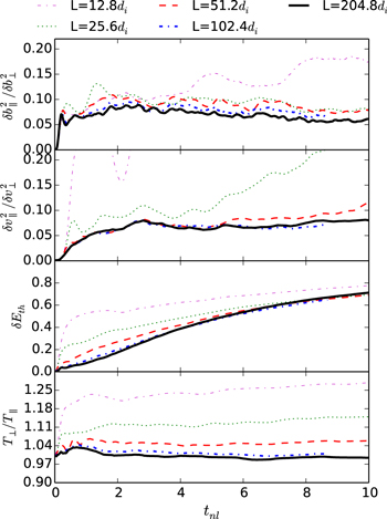
Figure 2. Variance anisotropy and plasma heating as functions of nominal nonlinear time. The top two panels show  and
and  ; the bottom two panels show proton heating and anisotropy of proton heating.
Download figure:
Standard image High-resolution imageTwo important features should be noted. First, both  and
and  rise from near zero in less than a nonlinear time and saturate to stable values within a couple of nonlinear times. Second, for both the
  and the
  fields, the relative parallel variances are larger for smaller systems and become smaller for larger system sizes. The values converge for larger system sizes to about 0.05. This level is not too different from typical reported solar wind observations (e.g., Belcher & Davis 1971; Leamon et al. 1998; Oughton et al. 2015).
The convergence of variance anisotropy to a stable value with increasing system size (or equivalently, Reynolds number) is reminiscent of the convergence to MHD-like behavior with system size as found by Parashar et al. (2015). This is clear in the bottom two panels of Figure 2. Proton heating  as well as proton thermal anisotropy saturate for larger system sizes
  . This corresponds to larger effective Reynolds number ∼1207 and is consistent with the view that at high Reynolds number the system approaches a state controlled by the dynamics of the large eddies that contain most of the energy.
To study the convergence of the variance anisotropy with system size, we calculate  , where Q is the quantity of interest (v or b or T anisotropy) and
  denotes time averaging over the period
  –8. "Sim" and "Smaller Sim" are two simulations of consecutive sizes, with "Sim" having a given Reynolds number Re and "Smaller Sim" having the next smaller value of Re; e.g., the
  and
and  , runs, respectively. Figure 3 plots these
  as a function of reciprocal Reynolds number, and provides a quantitative measure of the convergence we observe in Figure 2. The
  each follow (approximate) power laws, indicating a convergent behavior with increasing Reynolds number. This suggests that our largest system (
 ) is approaching asymptotic values of variance anisotropy and proton heating.
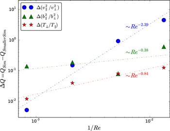
Figure 3. Convergence test for variance anisotropies and proton thermal anisotropy.  (the difference between time-averaged values of a quantity of interest Q for two consecutive simulations) plotted vs. an inverse Reynolds number (see text for details). Power-law fits are indicated by the dotted lines.
Download figure:
Standard image High-resolution imageEvidently, the above diagnostic is sensitive to the contributions to variance anisotropy from the largest energy-containing scales in the system. Figure 4 shows the ratio of energy in the parallel magnetic field component,  , to energy in the perpendicular magnetic component,
  , as a function of the perpendicular wavenumber,
  . The spectra are computed in the
  plane and summed over "rings" defined by
  (box units) to get the spectra as functions of
  .
.

Figure 4. Ratio of energy in parallel and perpendicular variance of magnetic field as a function of perpendicular wavenumber. The cyan-shaded area shows where the simulation noise is large and an artificially large electron to proton mass ratio may be skewing results. The dashed lines show the largest scales. The filled circles indicate the (box unit) wavenumbers  these were unpopulated in the initial condition. The stars indicate the (box unit) wavenumbers
  , which contained the initial conditions. The lines for ∣k∣ larger than the starred values (following the legend) show all larger wavenumbers populated by the cascade. The dotted curve with triangles is the ratio of power spectral densities extracted from the bottom panel of Figure 1 in Kiyani et al. (2013) converted to wavenumber space assuming Taylor's hypothesis.
Download figure:
Standard image High-resolution image
Indeed, in Figure 4 one can see that the average value of variance anisotropy at the larger, energy-containing scales in our larger simulations is close to the stable global values shown above in Figure 2 and is also comparable to the values obtained for larger scales in the solar wind observational study of Kiyani et al. (2013).
The data plotted in Figure 4 also allows us to explore the behavior of the variance anisotropy at scales that are populated by the cascade, i.e., scales empty in the initial conditions. Clearly, the largest wavelength fluctuations, which were initially absent, become populated through "backscatter" and attain values of  that are actually larger than the global average (the first circle in Figure 4). The next wavenumber, corresponding to two wavelengths in the box, was also unpopulated initially and has a very small parallel variance, lower than the global average, in all runs. The next several higher wavenumbers contained the initial conditions and these have relatively low values of parallel variance, but one begins to see an increase of
  moving toward higher k. At still higher wavenumbers, those which were unpopulated initially, we observe near monotonic increases of variance ratio. Overall, this suggests that as the cascade progresses toward smaller scales (e.g., Kiyani et al. 2013), the variance ratio or "magnetic compressibility" increases gradually. Note that the isotropic value (0.5) is marked in the figure by the horizontal dotted line. The cyan-shaded region identifies the wavenumbers numerically affected by artificially large electron mass (
 ) and/or noise associated with the finite number of PIC particles. Results in this region are heavily affected by these numerical constraints. In particular, in all cases the variance ratio approaches unity at high k, corresponding to equipartitioned noise due to counting statistics for these 2.5D simulations.
Also shown in Figure 4 are the ratios of parallel and perpendicular variances calculated by Kiyani et al. (2013) using CLUSTER data. This was from a fast wind interval with a proton plasma  , similar to that of our simulations. Kiyani et al. (2013) provided their results in the frequency domain; here their results are converted to wavenumber space using Taylor's hypothesis. The spacecraft data shows an interesting level of agreement with our larger simulations for scales approaching
  . Deeper in the kinetic regime, the simulations and data separate from each other. This is potentially because of both physical and numerical reasons, namely, the possible inapplicability of Taylor's hypothesis to observations at kinetic scales and the numerical issues alluded to above: particle noise and the artificially small scale-separation between protons and electrons (
 ) in the simulations. Surprisingly, the simulations and Kiyani et al. observational results are in approximate agreement in the decade
  , even though the simulations were not designed to specifically correspond to this solar wind interval. The similar values of
  may be the controlling factor (Oughton et al. 2016).
There is another issue: the interval of averaging that enters into comparison of our results with published observations. The analyses of Belcher & Davis (1971) and Leamon et al. (1998) employed relatively long intervals to compute variances, and hence can be treated as computations relative to a global mean field. However, the numbers reported by Kiyani et al. (2013) employed a "local mean field" that uses a small amount of data and also depends on the scale of interest. The local mean field approaches the global mean field when the scale of interest becomes large, but it may depart significantly from the global mean field for small scales (e.g. Matthaeus et al. 2012). This systematic effect might contribute to differences between our results and the Kiyani et al. (2013) results at scales smaller than di.
A more general view of the dependence of results on the size of averaging interval was given recently by Isaacs et al. (2015), who showed that the values of various quantities, including variance anisotropy of magnetic field, depend on the size of averaging interval. Averaging intervals of size comparable to correlation length appear to be optimal in order to avoid large variability.
4. DISCUSSION AND CONCLUSIONS
In this paper, we examined the emergence of parallel variance in the nonlinear dynamics of a kinetic plasma that is initiated with fluctuations that have only perpendicular variance or, more precisely, toroidal variance. The emergence of parallel variance—the fluctuating component of velocity or magnetic field that lies in the direction of the large-scale mean magnetic field—is of special significance in plasma dynamics. In a linear wave picture, the "Alfvén mode" is strictly transverse in the fluid limit (i.e., variance perpendicular to the mean magnetic field, and the wavevector) and represents a purely incompressive motion. Therefore, in the fluid regime (and still from a linear wave perspective), parallel variance indicates the presence of magnetosonic modes and introduces the possibility of compressive motions. For this reason, the parallel magnetic variance is often associated with "magnetic compressibility."
Of course parallel variance can be present in incompressible, compressible, and kinetic plasmas. In the special cases of purely incompressible MHD with a strong mean magnetic field and incompressible MHD in 2.5D, the parallel variance becomes passive. If it is present initially, it will be passively advected and if it is not present initially, it will not be generated (see e.g., the original derivations in Montgomery 1982 and Montgomery & Turner 1982, and later related works (e.g., Goldreich & Sridhar 1995; Maron & Goldreich 2001; Mason et al. 2006)). There are several families of reduced physics models in which parallel variance fluctuations are distinguished by their suppression or absence. Examples are reduced magnetohydrodynamics (RMHD), nearly incompressible MHD (NIMHD), and the Goldreich–Sridhar critical balance theory of MHD (CB). Of these, RMHD eliminates parallel variance as a requirement for low-frequency motions (Kadomtsev & Pogutse 1974; Strauss 1976). NIMHD describes the low Mach number approach to incompressibility and it transpires that this asymptotic limit requires the suppression of the parallel variance (Zank & Matthaeus 1992, 1993). The CB model emerges from a weak turbulence approach and an MHD wave mode representation. Because it is assumed that the pseudo-Alfvén modes have a negligible energy budget and do not interact with the shear Alfvén modes, the parallel variance is ordered out by construction (Goldreich & Sridhar 1995, 1997). A perusal of the derivations and assumptions underlying these models makes clear the assertion that parallel variance is associated with fast timescales or high frequencies and therefore accordingly with density compressions and non-solenoidal velocities. Consequently, the presence of significant parallel variance is connected with compressible behavior in a broad range of models and not only in linear wave theory.
An important conclusion of the present study is that for large plasmas—meaning those having a characteristic scale greater than a few tens of  —the parallel magnetic variance grows from zero amplitude to a level of 5% to 10% of the perpendicular magnetic variance and remains at approximately constant fractional levels thereafter. Similar conclusions hold for velocity variances. The timescale for reaching this steady level is a few nonlinear large-scale eddy turnover times,
  . Moreover, examination of the evolution of density fluctuations reveals that their characteristic timescale for growth is also
  . The noteworthy conclusion is that both parallel magnetic variance, parallel velocity variance, and the variance of the proton density evolve on hydrodynamic-like (MHD) timescales, and not on plasma timescales such as the gyroperiod.
We also note that while primitive (unaveraged) variables such as density must admit time variations on faster compressional (e.g., magnetosonic) timescales (not shown), such variations are not evident in the time evolution of the variances. This appears to lend some credence to the view that parallel variances are quasi-passive in certain limits. For example, this passivity is exact for incompressible 2.5D MHD (e.g., Montgomery & Turner 1982) and correct to first-order in perturbation theory in nearly incompressible MHD (Zank & Matthaeus 1993). However, the parallel variance cannot be completely passive and evolving independently of the transverse fluctuations as has been suggested in some studies (Goldreich & Sridhar 1995; Maron & Goldreich 2001; Cho et al. 2002). This full independence would clearly be inconsistent with the result found both here and in the companion (MHD-scale) study of Oughton et al. (2016) that parallel variance emerges dynamically from an Alfvénic polarization initial state and on timescales controlled by the large-scale nearly incompressible transverse Alfvénic fluctuations.
In conclusion, we showed that a turbulent kinetic plasma generates parallel variance as well as density fluctuations in about a system nonlinear time irrespective of Reynolds number. The levels of variance anisotropy converge to stable values for sufficiently large system size. These results indicate, in accord with our previous conclusions (Parashar et al. 2015), that to have an adequate representation of effects of the large-scale physics at kinetic scales, one needs a system size  (e.g., for the parameters of the present study,
  ). Systems of smaller size will have shortcomings. Somewhat remarkably for the larger system size simulations reported on here, the distribution of variance anisotropy over scales shows behavior similar to the solar wind for MHD scales. In particular, the ratio of parallel variance to perpendicular variance increases in the decade approaching
  from below.
Various additional aspects of the problem have not been addressed herein. The dependence on plasma β, Alfvén ratio, and different initial conditions in the context of compressible MHD is discussed in Oughton et al. (2016), and needs to be studied also in the kinetic limit. The numerical aspects of how resolution and geometry could affect the results will be discussed elsewhere. The level of anisotropy achieved often does not depend much on the initial conditions, as shown by Oughton et al. (2016), but might differ between decaying and driven runs, possibly depending on the nature of the driving.
This research was supported in part by NSF AGS-1063439 and AGS-1156094 (SHINE), and by NASA grants NNX15AB88G (LWS) and NNX14AI63G (Heliophysics Grand Challenges) as well as the Solar Probe Plus project under subcontract D99031L from the Southwest Research Institute ISOIS project and a subcontract from Space Science Institute on NSF grant AGS-1460130.