


ABSTRACT
The detection of a gamma-ray burst (GRB) in the solar neighborhood would have very important implications for GRB phenomenology. The leading theories for cosmological GRBs would not be able to explain such events. The final bursts of evaporating primordial black holes (PBHs), however, would be a natural explanation for local GRBs. We present a novel technique that can constrain the distance to GRBs using detections from widely separated, non-imaging spacecraft. This method can determine the actual distance to the burst if it is local. We applied this method to constrain distances to a sample of 36 short-duration GRBs detected by the Interplanetary Network (IPN) that show observational properties that are expected from PBH evaporations. These bursts have minimum possible distances in the 1013–1018 cm (7–105 au) range, which are consistent with the expected PBH energetics and with a possible origin in the solar neighborhood, although none of the bursts can be unambiguously demonstrated to be local. Assuming that these bursts are real PBH events, we estimate lower limits on the PBH burst evaporation rate in the solar neighborhood.
Export citation and abstract BibTeX RIS
1. INTRODUCTION
The composition of the short-duration, hard-spectrum gamma-ray burst (GRB) population is not yet fully understood. It is believed that most of the bursts are generated in compact binary mergers (Eichler et al. 1989) and while the handful of optical counterparts and host galaxies discovered to date does not contradict this view, it is also thought that the population probably contains up to 8% extragalactic giant magnetar flares as well (Mazets et al. 2008; Hurley et al. 2010; Svinkin et al. 2015). For the majority of the short-duration GRB population, however, there is simply not enough evidence to determine their origin unambiguously. Hawking radiation from primordial black holes (PBH) was one of the very first explanations proposed for cosmic GRBs (Hawking 1974), and it continues to be proposed today (Cline & Hong 1996; Cline et al. 1997, 1999, 2003, 2005; Czerny et al. 2011). The PBH lifetime and burst duration depend on its mass, so that PBHs bursting today have similar masses and durations, and release similar energies, making them in essence "standard candles." The typical PBH GRB is not expected to be accompanied by detectable, intrinsically generated extended emission (EE) or to have an afterglow, although accompanying bursts at other wavelengths or afterglows may arise if, for example, the PBH is embedded in a high-density magnetic field or plasma (Jelley et al. 1977; Rees 1977; MacGibbon et al. 2008). In the standard emission scenario, so called because it uses the Standard Model of particle physics (MacGibbon & Webber 1990), the PBH GRB is strongest in the final second of the burst lifetime, has a hard energy spectrum, and should be detectable in the vicinity of the Earth. For a typical interplanetary network (IPN) detector sensitive to bursts of fluence 10−6 erg cm−2 and above, PBH events could in principle be detected out to a distance of a few parsecs depending on the emission model. PBHs evaporating today do not have sufficient luminosity to be detected at cosmological distances even by the most sensitive current instruments, and so searching for them locally is a logical step.
When observed by a single detector, the properties of a PBH burst might not appear to be significantly different from those of other short bursts; instruments with localization or imaging capabilities would obtain their arrival directions as they would for an infinitely distant source. Indeed, many attempts to find evidence for the existence of PBH bursts to date have been based mainly on the spatial distribution and time histories of a subset of short bursts (Cline & Hong 1996; Cline et al. 1997, 1999, 2003, 2005; Czerny et al. 2011). Other search methods have employed atmospheric Cherenkov detectors (Porter & Weekes 1977, 1978, 1979; Linton et al. 2006; Tesic & VERITAS Collaboration 2012; Glicenstein et al. 2013), air shower detectors (Fegan et al. 1978; Bhat et al. 1980; Alexandreas et al. 1993; Amenomori et al. 1995; Abdo et al. 2015), radio pulse detection (Phinney & Taylor 1979; Keane et al. 2012), spark chamber detection (Fichtel et al. 1994), and GRB femtolensing (Barnacka et al. 2012). Table 1 gives a comparison of these various methods.
Table 1. Comparison of Methods Used to Detect PBH Evaporations
| Method | Burst Duration (s) | Energy or Frequency | Rate Upper Limits (pc−3 yr−1) | References |
|---|---|---|---|---|
| Atmospheric Cherenkov | 10−7–0.1 | 200 Mev–10 TeV | 0.04–8.7 × 10⁵ | 1 |
| Air Shower | 10−6–0.1 | 5 × 10¹²–≳5 × 10¹³ eV | 2.7 × 10³–6 × 10³ | 2 |
| Radio Pulse | <3 × 10⁻³ | 430–1374 MHz | 2 × 10⁻⁹ | 3 |
| Spark Chamber | 10−6 | 20 MeV–1 GeV | 5 × 10⁻² | 4 |
| Spatial Distribution | <0.1 | 15 keV–10 MeV | ... | 5 |
References. (1) Porter & Weekes (1977, 1978, 1979), Abdo et al. (2015), (2) Bhat et al. (1980), Fegan et al. (1978), (3) Phinney & Taylor (1979), Keane et al. (2012), (4) Fichtel et al. (1994), (5) Cline & Hong (1996), Cline et al. (1997, 1999, 2003, 2005); Czerny et al. (2011).
Download table as: ASCIITypeset image
To widely spaced IPN detectors, however, a local PBH burst could look significantly different when compared with bursts from distant sources due to the curvature of the received wavefront. In this paper, we use this fact to explore the possibility that some short bursts may originate in the solar neighborhood, and estimate lower limits to the PBH burst evaporation rate assuming that these bursts are real PBH bursts. This paper is organized as follows. In Section 2, we derive the fluence expected in the detector from a PBH burst using the standard emission model (SEM) and, as a maximal alternative, the Hagedorn emission model. In Section 3, we explain how we localized the detected bursts in three dimensions, relaxing the assumption that they are at infinite distances. The detailed discussion of the methodology is given in the
2. PBH BURST SIGNATURES
As a PBH Hawking-radiates, its mass is decreased by the total energy carried off by the emission and the black hole temperature, which is inversely proportional to its mass, increases. In the SEM (MacGibbon & Webber 1990), the black hole directly Hawking-radiates those particles which appear to be fundamental on the scale of the black hole. Once the black hole temperature reaches the QCD transition scale (∼200–300 MeV), quarks and gluons are directly Hawking-radiated. The PBH GRB spectrum is the combination of the directly Hawking-radiated photons and those produced by the decay of other directly Hawking-radiated particles. An SEM PBH with a remaining emission lifetime of τ ≲ 1 s has a mass of
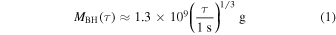
(Ukwatta et al. 2016) and a remaining rest-mass energy of

The expected fluence arriving at the detector from a PBH at a distance d from Earth is then

where  and
and  is the fraction of the PBH energy that arrives in the energy band of the detector, and the maximum distance from which the SEM PBH is detectable is
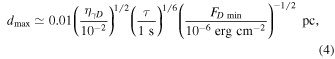
where  is the sensitivity of the detector.
The SEM analysis is consistent with high-energy accelerator experiments (MacGibbon et al. 2008). However, an alternative class of PBH evaporation models was proposed before the existence of quarks and gluons was confirmed in accelerator experiments, and these models continue to be discussed in the PBH burst literature. In such models (which we label HM scenarios), a Hagedorn-type exponentially increasing number of degrees of freedom becomes available as radiation modes once the black hole temperature reaches a specific threshold, such as the QCD transition scale. In the HM scenarios, we assume that the remaining PBH mass is emitted quasi-instantaneously as a burst of energy  once the black hole mass reaches some threshold
  for the QCD transition scale,
  g and
g and  erg. Proceeding as above, the maximum distance from which the HM PBH burst is detectable is
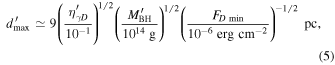
where  is the fraction of the HM PBH energy that arrives in the energy band of the detector.
3. GAMMA-RAY BURST LOCALIZATION FOR A SOURCE AT A FINITE DISTANCE
When a pair of IPN spacecraft detects a burst (Figures 1 and 2), if the distance to the source is taken to be a free parameter, then the event is localized to one sheet of a hyperboloid of revolution about the axis defined by the line between the spacecraft. If the burst is assumed to be at a distance which is much greater than the interspacecraft distance, the hyperboloid intersects the celestial sphere to form the usual localization circle (or annulus, when uncertainties are taken into account). Another widely spaced spacecraft would produce a second hyperboloid that intersects the first one to define a locus of points which is a simple hyperbola. Note that both hyperboloids have a common focus. Again, if the burst is assumed to be at a large distance from the spacecraft, then the hyperbola intersects the celestial sphere at two points to define two possible error boxes. A fourth, non-coplanar spacecraft, even at a moderate distance from Earth, such as Konus-WIND, can often be used to eliminate one branch of the hyperbola and part of the second branch. A terrestrial analog to this method is the time difference of arrival, with the important exception that GRB sources can be at distances which are effectively infinite. Further details are given in the

Figure 1. Two-dimensional example of GRB triangulation when the source distance is allowed to vary. The two spacecraft, 1 and 2, are aligned along the z-axis, and are the foci of a hyperbola. The hyperbola defines the loci of the possible source distances. If the distance is assumed to be infinite, the two possible GRB arrival directions are along the asymptotes (dashed lines).
Download figure:
Standard image High-resolution image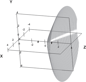
Figure 2. Hyperbola of Figure 1 rotated to obtain one sheet of a hyperboloid of rotation of two sheets. The two spacecraft are aligned along the z-axis and are the foci of the hyperboloids. Each hyperboloid defines the loci of possible source distances in the three-dimensional problem. If the distance is assumed to be infinite, then the circle defined by the intersection of the hyperboloid with the celestial sphere gives the possible GRB arrival directions.
Download figure:
Standard image High-resolution imageIn this paper, we relax the assumption that bursts are at infinite distances. If a burst is detected by three widely spaced spacecraft, then according to the previous discussion, the possible location of the burst traces a simple hyperbola in space as illustrated in Figure 3. In an Earth-centered coordinate system, this hyperbola has a closest distance to the Earth, that is, a distance lower limit. As we explain in Section 5.2, this fact can be used to calculate a lower limit to the PBH burst density rate in the Solar neighborhood assuming that the bursts that we consider are actual PBH bursts. In principle, detections by three spacecraft can rule out a local origin for a burst, but it is impossible to prove a local origin with only three non-imaging spacecraft.
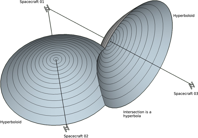
Figure 3. Intersection of two hyperboloids. With detections from three spacecraft, each spacecraft pair constrains the location of the source to a surface of a hyperboloid. The intersection of the two hyperboloids is a simple hyperbola contained in a plane. The point on this hyperbola that is closest to Earth gives the lower limit to the source distance.
Download figure:
Standard image High-resolution imageIn the case where a burst is observed by four widely spaced non-imaging spacecraft, the burst can be localized to a single point in space (or a region in space if uncertainties are taken into consideration). This scenario is illustrated in Figure 4. Thus, in order to prove the local origin of a burst using non-imaging spacecraft, one needs detections from at least four satellites that are at interplanetary distances from each other.
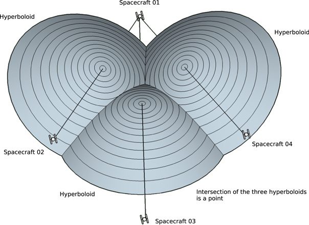
Figure 4. Intersection of three hyperboloids. Using detections with four widely separated spacecraft, each spacecraft pair constrains the location of the source to a surface of a hyperboloid. The intersection of the three hyperboloids is a point in space as illustrated in the figure. In this case, one can determine the source distance purely by timing measurements.
Download figure:
Standard image High-resolution imageAs mentioned in the
4. DATA SELECTION
The IPN database contains information on over 25,000 cosmic, solar, and magnetar events which occurred between 1990 and the present (http://ssl.berkeley.edu/ipn3/index.html). During this period, a total of 18 spacecraft participated in the network. Some were dedicated GRB detectors, while others were primarily gamma-ray detectors with GRB detection capability. Indeed, the composition of the IPN changed regularly during this time, as old missions were retired and new ones were launched. However, all of the instruments were sensitive to bursts with fluences around 10−6 erg cm−2 or peak fluxes of 1 photon cm−2 s−1 and above, resulting in a roughly constant detection rate. All of the known bursts, regardless of their intensity or duration, or the instruments which detected them, are included in this list. We have searched this list for GRBs with the following properties.
- 1.Confirmed cosmic bursts which occurred between 1990 October and 2014 December (24.25 years; 10,795 GRBs survived this cut).
- 2.Bursts observed by three or more spacecraft, of which two were at interplanetary distances (839 GRBs survived this cut). This small number is due first to the relatively high sensitivity thresholds of the distant IPN detectors (roughly 10−6 erg cm−2 or 1 photon cm−2 s−1) and their somewhat coarser time resolutions, and second to a 2.5 year period between 1993 August and 1996 February when there was only one interplanetary spacecraft in the network.
- 3.Bursts with no X-ray or optical afterglow, either because there were no follow-up observations or because searches were negative. In addition, as discussed before, the arrival direction derived from IPN localization depends on its assumed distance, and the bursts were initially triangulated assuming an infinite distance. Thus, even if a simultaneous search had taken place, it might not have identified an event within the error box if the burst was local. Other selection effects come into play starting with the launch of the HETE spacecraft in 2000 October, and later with the launch of Swift in 2004 November, namely, that X-ray and optical observations were often performed rapidly, leading to more X-ray and optical detections and the elimination of the bursts from further consideration here. On the other hand, the launch of Suzaku in 2005 July and of Fermi in 2008 June resulted in an increase in the short burst detection rate which more than compensated for the previous effect.
- 4.Bursts with durations <1 s and no EE. No cut was made based on the light curve shape; we discuss this in Section 6. The detection rate of short bursts was roughly, but not exactly, constant over the period of this study.
These cuts, which are commutative, were carried out in the order described above, so as to minimize the required analysis of the full sample of 10,795 events. Thirty-six bursts satisfied these criteria. None were detected by an imaging instrument with good spatial resolution. While we believe that the overall IPN detection rate of short bursts was roughly constant, the data selection resulted in a rate which varied significantly from year to year.
In order to obtain distance lower limits as described in
Table 2. Distance Lower Limits for IPN Gamma-ray Bursts
| GRB | SOD | Spacecrafta | Dur. | Fluence | Energy | Minimum | Maximum | Maximum | Maximum | Counterpart | References |
|---|---|---|---|---|---|---|---|---|---|---|---|
| (s) | (erg cm−2) | Range | Distance | Detectable | Detectable | Detectable | Search? | ||||
| (keV) | (cm) | dist. (cm) | dist. ( cm) cm) |
dist. ( cm) cm) |
|||||||
| (SEM Model) | (HM Model) | ||||||||||
| 910206 | 31529 | Uly, PVO, Phe | 0.7 | 1.1 × 10⁻⁵ | 100–100000 | 1.8 × 10¹⁴ | 8.5 × 10¹⁸ | 8.8 × 10¹⁶ | 2.6 × 10¹⁹ | No | 1, 6 |
| 920414 | 84162 | Uly, BAT, PVO | 0.96 | 5.8 × 10⁻⁶ | 20–2000 | 6.7 × 10¹³ | 1.2 × 10¹⁹ | 1.3 × 10¹⁷ | 3.7 × 10¹⁹ | No | 2, 3, 6 |
| 970902 | 27561 | Uly, Kon, NEAR | 0.44 | 4.2 × 10⁻⁶ | 10–10000 | 1.3 × 10¹³ | 1.4 × 10¹⁹ | 1.3 × 10¹⁷ | 4.3 × 10¹⁹ | No | 4, 5 |
| 970921 | 83828 | Uly, Kon, NEAR | 0.06 | 2.9 × 10⁻⁶ | 10–10000 | 9.0 × 10¹⁴ | 1.6 × 10¹⁹ | 1.1 × 10¹⁷ | 5.1 × 10¹⁹ | No | 4, 5 |
| 981102 | 28554 | Uly, Kon, NEAR | 0.57 | 1.1 × 10⁻⁵ | 10–10000 | 1.5 × 10¹⁴ | 8.5 × 10¹⁸ | 8.5 × 10¹⁶ | 2.7 × 10¹⁹ | No | 5, 13 |
| 990712 | 27919 | Uly, BAT, Kon, NEAR | 0.62 | 2.1 × 10⁻⁵ | 10–10000 | 2.8 × 10¹⁶ | 1.3 × 10¹⁹ | 6.2 × 10¹⁶ | 1.9 × 10¹⁹ | No | 5, 8 |
| 000607 | 08689 | Uly, Kon, NEAR | 0.09 | 4.6 × 10⁻⁶ | 10–10000 | 2.7 × 10¹³ | 1.4 × 10¹⁹ | 9.6 × 10¹⁶ | 4.1 × 10¹⁹ | 14, 15 | 5, 13 |
| 001025 | 71369 | Uly, Kon, NEAR | 0.48 | 4.9 × 10⁻⁶ | 10–10000 | 7.0 × 10¹³ | 1.4 × 10¹⁹ | 1.2 × 10¹⁷ | 4.0 × 10¹⁹ | 15, 16 | 5, 13 |
| 001204 | 28869 | Uly, Kon, SAX, NEAR | 0.27 | 1.1 × 10⁻⁶ | 10–10000 | 4.4 × 10¹³ | 3.0 × 10¹⁹ | 2.4 × 10¹⁷ | 8.4 × 10¹⁹ | 15, 17, 18 | 5, 7, 13 |
| 010104 | 62490 | Uly, Kon, SAX, NEAR | 0.76 | 6.6 × 10⁻⁷ | 10–10000 | 7.8 × 10¹³ | 3.6 × 10¹⁹ | 3.6 × 10¹⁷ | 1.1 × 10²⁰ | No | 5, 7, 13 |
| 010119 | 37177 | Uly, Kon, NEAR | 0.18 | 2.3 × 10⁻⁶ | 10–10000 | 2.8 × 10¹³ | 1.9 × 10¹⁹ | 1.5 × 10¹⁷ | 5.8 × 10¹⁹ | No | 5, 7, 13 |
| 080203 | 08456 | Ody, Kon, INT, MES | 0.4 | 9.3 × 10⁻⁶ | 10–10000 | 1.5 × 10¹⁷ | 9.8 × 10¹⁸ | 8.7 × 10¹⁶ | 2.9 × 10¹⁹ | No | 5, 13 |
| 080222 | 37262 | Ody, Kon, MES | 0.11 | 1.9 × 10⁻⁶ | 10–10000 | 4.0 × 10¹³ | 2.1 × 10¹⁹ | 1.6 × 10¹⁷ | 6.4 × 10¹⁹ | No | 5, 13 |
| 080530 | 58296 | Ody, INT, MES, Suz | 0.41 | 1.0 × 10⁻⁶ | 100–1000 | 1.6 × 10¹³ | 2.8 × 10¹⁹ | 2.6 × 10¹⁷ | 8.7 × 10¹⁹ | No | 6 |
| 090228 | 17600 | Ody, Kon, RHE, MES | 0.08 | 6.3 × 10⁻⁶ | 10–10000 | 2.9 × 10¹³ | 1.1 × 10¹⁹ | 8.1 × 10¹⁶ | 3.5 × 10¹⁹ | No | 5, 6, 9, 10, 19 |
| 090523 | 34075 | Ody, Kon, MES, Suz | 0.5 | 1.6 × 10⁻⁶ | 10–10000 | 6.2 × 10¹⁶ | 2.3 × 10¹⁹ | 2.2 × 10¹⁷ | 6.9 × 10¹⁹ | No | 5, 6, 13 |
| 100223 | 09491 | Ody, Kon, MES, Suz | 0.19 | 1.7 × 10⁻⁶ | 10–10000 | 8.8 × 10¹³ | 2.3 × 10¹⁹ | 1.8 × 10¹⁷ | 6.7 × 10¹⁹ | No | 5, 6, 9, 10 |
| 100629 | 69243 | Ody, Kon, INT, MES | 0.46 | 1.1 × 10⁻⁶ | 10–10000 | 4.3 × 10¹⁴ | 2.6 × 10¹⁹ | 2.6 × 10¹⁷ | 8.5 × 10¹⁹ | No | 5, 6, 9, 10 |
| 100811 | 09349 | Ody, Kon, INT, MES | 0.33 | 4.4 × 10⁻⁶ | 10–10000 | 6.5 × 10¹⁴ | 1.6 × 10¹⁹ | 1.2 × 10¹⁷ | 4.2 × 10¹⁹ | No | 5, 6, 9, 11 |
| 101009 | 24858 | Ody, Kon, INT, MES | 0.18 | 1.6 × 10⁻⁶ | 10–10000 | 4.6 × 10¹⁵ | 1.6 × 10¹⁹ | 1.8 × 10¹⁷ | 6.9 × 10¹⁹ | No | 5, 6, 13 |
| 101129 | 56371 | Ody, Kon, INT, MES | 0.32 | 3.7 × 10⁻⁶ | 10–10000 | 3.9 × 10¹³ | 3.0 × 10¹⁹ | 1.3 × 10¹⁷ | 4.6 × 10¹⁹ | No | 5, 9, 11 |
| 110510 | 80844 | Ody, Kon, Swi, MES | 0.84 | 9.7 × 10⁻⁷ | 10–10000 | 2.6 × 10¹⁵ | 3.1 × 10¹⁹ | 3.0 × 10¹⁷ | 8.9 × 10¹⁹ | No | 6, 13 |
| 110705 | 13031 | Ody, Kon, INT, MES | 0.22 | 5.7 × 10⁻⁶ | 10–10000 | 3.2 × 10¹⁵ | 1.7 × 10¹⁹ | 1.0 × 10¹⁷ | 3.7 × 10¹⁹ | No | 9, 11, 20, 21, 22 |
| 110802 | 55157 | Ody, Kon, INT, MES | 0.54 | 1.3 × 10⁻⁵ | 10–10000 | 3.0 × 10¹⁵ | 7.8 × 10¹⁸ | 7.6 × 10¹⁶ | 2.4 × 10¹⁹ | No | 13, 23, 24 |
| 120222 | 01776 | Ody, Kon, MES, Fer | 0.87 | 1.8 × 10⁻⁶ | 10–10000 | 5.5 × 10¹⁵ | 2.1 × 10¹⁹ | 2.3 × 10¹⁷ | 6.6 × 10¹⁹ | No | 9, 11 |
| 120519 | 62294 | Ody, Kon, MES, Fer | 0.91 | 3.6 × 10⁻⁶ | 10–10000 | 1.4 × 10¹⁵ | 1.8 × 10¹⁹ | 1.6 × 10¹⁷ | 4.6 × 10¹⁹ | No | 9, 11, 25, 26, 27 |
| 120811 | 01230 | Ody, Kon, MES, Fer | 0.31 | 4.3 × 10⁻⁶ | 10–10000 | 1.1 × 10¹⁴ | 1.9 × 10¹⁹ | 1.2 × 10¹⁷ | 4.2 × 10¹⁹ | No | 9, 11, 28, 29, 30, 31 |
| 121023 | 27857 | Ody, MES, Fer | 0.51 | 7.7 × 10⁻⁷ | 10–1000 | 9.2 × 10¹⁵ | 3.2 × 10¹⁹ | 3.1 × 10¹⁷ | 1.0 × 10²⁰ | No | 9, 11 |
| 121127 | 78960 | Ody, Kon, INT, MES | 0.53 | 2.8 × 10⁻⁶ | 10–10000 | 5.6 × 10¹⁴ | 4.1 × 10¹⁹ | 1.7 × 10¹⁷ | 5.3 × 10¹⁹ | No | 11, 12, 32, 33, 34 |
| 130501 | 00831 | Ody, Kon, MES, Suz | 0.41 | 2.0 × 10⁻⁶ | 10–10000 | 7.7 × 10¹³ | 2.0 × 10¹⁹ | 1.9 × 10¹⁷ | 6.2 × 10¹⁹ | No | 13 |
| 130504B | 27123 | Ody, Kon, MES | 0.36 | 8.8 × 10⁻⁶ | 10–10000 | 3.2 × 10¹³ | 9.2 × 10¹⁸ | 8.8 × 10¹⁶ | 3.0 × 10¹⁹ | No | 35, 36, 37, 38 |
| 131126A | 14050 | Ody, Kon, MES, Fer | 0.12 | 2.3 × 10⁻⁶ | 10–10000 | 3.1 × 10¹⁴ | 2.0 × 10¹⁹ | 1.4 × 10¹⁷ | 5.8 × 10¹⁹ | 39 | 40, 41, 42 |
| 140414B | 80735 | Ody, Kon, INT, MES | 0.97 | 2.3 × 10⁻⁶ | 10–10000 | 3.7 × 10¹⁴ | 2.0 × 10¹⁹ | 2.0 × 10¹⁷ | 5.9 × 10¹⁹ | No | 13 |
| 140807 | 43173 | Ody, Kon, MES, Fer | 0.57 | 2.6 × 10⁻⁶ | 10–10000 | 1.5 × 10¹⁸ | 1.8 × 10¹⁹ | 1.8 × 10¹⁷ | 5.5 × 10¹⁹ | 43 | 13 |
| 140906C | 85869 | Ody, Kon, INT, MES | 0.13 | 2.3 × 10⁻⁶ | 10–10000 | 1.3 × 10¹⁷ | 1.9 × 10¹⁹ | 1.5 × 10¹⁷ | 5.8 × 10¹⁹ | No | 44, 45 |
| 141011A | 24380 | Ody, Kon, MES, Fer | 0.06 | 1.4 × 10⁻⁶ | 10–10000 | 6.0 × 10¹³ | 2.5 × 10¹⁹ | 1.6 × 10¹⁷ | 7.3 × 10¹⁹ | No | 46, 47, 48 |
Note.
aFer: Fermi, INT: International Gamma-Ray Laboratory, Kon: Konus-Wind, MES: Mercury Surface, Space Environment, Geochemistry, and Ranging mission, NEAR: Near Earth Asteroid Rendezvous mission, Ody: Mars Odyssey, Phe: Phebus, PVO: Pioneer Venus Orbiter, RHE: Ramaty High Energy Solar Spectroscopic Imager, SAX: Satellite per Astronomia X (BeppoSAX), Suz: Suzaku, Swi: Swift (burst was outside the coded field of view of the BAT, and not localized by it), Uly: Ulysses.References. (1) Terekhov et al. (1994), (2) Goldstein et al. (2013), (3) Paciesas et al. (1999), (4) http://www.ioffe.ru/LEA/shortGRBs/Catalog/, (5) Pal'shin et al. (2013), (6) http://ssl.berkeley.edu/ipn3/index.html, (7) Frontera et al. (2009), (8) http://www.batse.msfc.nasa.gov/batse/grb/catalog/current, (9) Goldstein et al. (2012), (10) Paciesas et al. (2012), (11) von Kienlin et al. (2014), (12) Goldstein et al. (2012), (13) D. Svinkin et al. (2015, in preparation), (14) Masetti et al. (2000), (15) Hurley et al. (2002), (16) Park et al. (2000), (17) Price et al. (2000), (18) Vreeswijk & Rol (2000), (19) Guiriec et al. (2010), (20) Golenetskii et al. (2011d), (21) Golenetskii et al. (2011a), (22) Yasuda et al. (2011), (23) Hurley et al. (2011), (24) Golenetskii et al. (2011b), (25) Golenetskii et al. (2012d), (26) Golenetskii et al. (2012a), (27) Sakamoto et al. (2012), (28) Golenetskii et al. (2012e), (29) Golenetskii et al. (2012b), (30) Golenetskii et al. (2012f), (31) Xiong & Meegan (2012), (32) Golenetskii et al. (2012g), (33) Golenetskii et al. (2012c), (34) Ishida et al. (2012), (35) Vreeswijk & Rol (2000), (36) Golenetskii et al. (2013c), (37) Golenetskii et al. (2013a), (38) Yasuda et al. (2013), (39) Singer et al. (2013), (40) Golenetskii et al. (2013d), (41) Golenetskii et al. (2013b), (42) Pelassa & Meegan (2013), (43) L. Singer (2014, private communication), (44) Golenetskii et al. (2014c), (45) Golenetskii et al. (2014a), (46) von Kienlin (2014), (47) Golenetskii et al. (2014d), (48) Golenetskii et al. (2014b).
Download table as: ASCIITypeset image
Of the 10,795 GRBs which survived the first cut, we would expect roughly 20%, or 2150, to be short-duration events (<1 s). Of those, perhaps 10%, or 215, would display EE (Pal'shin et al. 2013), bringing the sample to 1935 non-EE bursts. We would expect about 80% of them to have no optical counterpart, either because none was detected or none was searched for (this number applies only to short bursts). This reduces the sample to about 1550. Since only 36 events survived all of the data cuts, we can estimate the average IPN efficiency for this selection procedure to be about 2.3%. Thus, if we exclude the 2.5 year period when the IPN had a single interplanetary spacecraft, then the observed event rate is 1.7 yr−1 and the true rate is about 72 yr−1.
5. RESULTS
5.1. Distance Limits and Localizations of PBH Burst Candidates
According to the methodology described in Section 3 and the
- 1.the date of the burst, in yymmdd format, with suffix A or B where appropriate;
- 2.the universal Time of the burst at Earth, in seconds of day;
- 3.the spacecraft which were used for the triangulation (a complete list of the spacecraft which detected the burst may be found on the IPN website, http://ssl.berkeley.edu/ipn3/index.html);
- 4.the burst duration, in seconds;
- 5.the fluence of the burst in erg cm−2;
- 6.the energy range over which the duration and fluence were measured, in keV;
- 7.the lower limit to the burst distance, obtained by triangulation, in cm;
- 8.the distance to which this burst could have been detected if it were a PBH burst of energy 1034 erg, assuming that all the energy went into the measured fluence (this is essentially the maximum possible detectable distance);
- 9.the maximum detectable distance assuming the SEM model (Equation (4)) in terms of the undetermined parameter
 ;
; - 10.the maximum detectable distance assuming the HM model (Equation (5)) in terms of the undetermined parameter;
- 11.whether or not counterpart searches took place and, if so, their references;
- 12.references to the duration, peak flux, and/or fluence measurements, and/or to the localization.


The shortest burst in Table 2 has a duration of 60 ms. Due to the relatively coarse time resolutions of interplanetary detectors, bursts with shorter durations must have greater intensities to be detected, effectively setting a higher detection threshold for very short events. The weakest event has a fluence of 4.65 × 10⁻⁷ erg cm−2. The bursts in Table 2 could not have come from distances less than the distance lower limits in column 7; however, all of them have time delays which are also consistent with infinite distances. Figure 5 shows a histogram of these minimum distances. The detector-dependent distance upper limits in column 8 are calculated assuming the extreme case that these events are caused by ∼1034 erg HM-type bursts from PBHs of mass ∼1014 g and that all of the emitted energy spectrum is contained within the detector measurement limits. Table 3 gives the coordinates of the centers and corners of the error boxes for the events in Table 2, assuming that the sources are at infinity. If the sources are in fact local, then the arrival directions are distance-dependent and different from those in Table 3. These coordinates represent the intersections of annuli, and in some cases the curvature of the annuli would make it inaccurate to construct an error box by connecting the coordinates with straight-line segments.
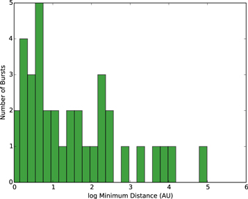
Figure 5. Histogram of the minimum distances to the PBH burst candidates in the IPN sample.
Download figure:
Standard image High-resolution imageTable 3. Localizations of IPN Gamma-ray Bursts Assuming Infinite Distances
| GRB | α | δ |
|---|---|---|
| 910206 | ||
| Center | 87.5650 | 17.3372 |
| Corners | 86.7457 | 17.8617 |
| 88.4371 | 16.5674 | |
| 86.6713 | 18.2592 | |
| 88.3683 | 16.9025 | |
| OR | ||
| Center | 86.9621 | 36.1678 |
| Corners | 86.0419 | 35.5941 |
| 87.9516 | 36.9783 | |
| 85.9902 | 35.1926 | |
| 87.8875 | 36.6407 | |
| 920414 | ||
| Center | 90.5234 | −76.3115 |
| Corners | 90.6025 | −76.3287 |
| 90.3189 | −76.2150 | |
| 90.7309 | −76.4079 | |
| 90.4446 | −76.2943 | |
| 970902 | ||
| Center | 351.0259 | +7.3294 |
| Corners | 351.0744 | +7.3080 |
| 351.1009 | +7.3100 | |
| 350.9774 | +7.3507 | |
| 350.9509 | +7.3486 | |
| 970921 | ||
| Center | 235.8826 | −24.8310 |
| Corners | 236.0899 | −24.3906 |
| 236.2034 | −24.1627 | |
| 235.6864 | −25.2436 | |
| 235.5867 | −25.4367 | |
| 981102 | ||
| Center | 277.0514 | −48.3354 |
| Corners | 277.0532 | −48.3258 |
| 277.0159 | −48.2744 | |
| 277.0496 | −48.3449 | |
| 277.0870 | −48.3962 | |
| 990712 | ||
| Center | 123.4627 | +6.6755 |
| Corners | 123.8544 | +7.2952 |
| 123.2666 | +6.3351 | |
| 123.2036 | +6.2494 | |
| 123.7301 | +7.1201 | |
| OR | ||
| Center | 125.3550 | +9.4408 |
| Corners | 124.9180 | +8.8500 |
| 125.6024 | +9.7478 | |
| 125.6597 | +9.8378 | |
| 125.0364 | +9.0294 | |
| 000607 | ||
| Center | 38.4971 | +17.1419 |
| Corners | 38.4656 | +17.1016 |
| 38.5472 | +17.2317 | |
| 38.5287 | +17.1823 | |
| 38.4470 | +17.0523 | |
| 001025 | ||
| Center | 275.3488 | −5.1067 |
| Corners | 275.4272 | −5.1411 |
| 275.1851 | −4.9912 | |
| 275.2707 | −5.0723 | |
| 275.5140 | −5.2229 | |
| 001204 | ||
| Center | 40.2997 | +12.8817 |
| Corners | 40.2796 | +12.8928 |
| 40.3478 | +12.8979 | |
| 40.3199 | +12.8707 | |
| 40.2516 | +12.8656 | |
| 010104 | ||
| Center | 317.3689 | +63.5116 |
| Corners | 317.6201 | +63.5227 |
| 317.5851 | +63.4776 | |
| 317.1183 | +63.5004 | |
| 317.1523 | +63.5455 | |
| 010119 | ||
| Center | 283.4446 | +11.9964 |
| Corners | 283.4892 | +12.0007 |
| 283.4159 | +11.9832 | |
| 283.4000 | +11.9921 | |
| 283.4734 | +12.0096 | |
| 080203 | ||
| Center | 48.2086 | +24.3289 |
| Corners | 48.1704 | +24.3216 |
| 48.2401 | +24.0161 | |
| 49.1541 | +20.8021 | |
| 48.9850 | +21.5848 | |
| 48.2469 | +24.3362 | |
| 47.7229 | +27.1306 | |
| 47.5349 | +27.9115 | |
| 48.1002 | +24.6272 | |
| 080222 | ||
| Center | 68.7192 | +56.9390 |
| Corners | 69.2723 | +57.0738 |
| 68.1039 | +56.6937 | |
| 68.1686 | +56.7979 | |
| 69.3407 | +57.1754 | |
| 080530 | ||
| Center | 5.3443 | 28.2246 |
| Corners | 5.2701 | 28.3257 |
| 5.4170 | 28.1570 | |
| 5.2717 | 28.2920 | |
| 5.4186 | 28.1232 | |
| 090228 | ||
| Center | 98.7014 | −28.7863 |
| Corners | 98.7827 | −28.8531 |
| 98.5307 | −28.6112 | |
| 98.5698 | −28.6709 | |
| 98.8219 | −28.9123 | |
| 090523 | ||
| Center | 22.8383 | −62.2047 |
| Corners | 23.0738 | −62.1859 |
| 23.2792 | −62.2169 | |
| 22.6023 | −62.2230 | |
| 22.3971 | −62.1907 | |
| 100223 | ||
| Center | 101.6711 | +12.8302 |
| Corners | 101.9024 | +12.6261 |
| 101.4091 | +13.4941 | |
| 101.5176 | +12.9034 | |
| 102.0085 | +12.0774 | |
| 100629 | ||
| Center | 227.6190 | +29.5479 |
| Corners | 227.6295 | +29.2934 |
| 227.5705 | +29.7415 | |
| 227.6081 | +29.8012 | |
| 227.6671 | +29.3536 | |
| 100811 | ||
| Center | 344.9605 | +20.6223 |
| Corners | 344.9395 | +20.5411 |
| 345.0289 | +20.6525 | |
| 344.9816 | +20.7032 | |
| 344.8922 | +20.5919 | |
| 101009 | ||
| Center | 75.6068 | −33.9325 |
| Corners | 75.8367 | −33.8146 |
| 76.0209 | −33.6624 | |
| 75.1904 | −34.1986 | |
| 75.3765 | −34.0492 | |
| 101129 | ||
| Center | 268.6211 | −7.7232 |
| Corners | 272.2014 | −9.1377 |
| 265.1168 | −6.9176 | |
| 272.2546 | −9.3668 | |
| 265.1792 | −7.0998 | |
| 110510 | ||
| Center | 336.1407 | −44.0726 |
| Corners | 344.4202 | −52.3621 |
| 344.5801 | −52.3041 | |
| 327.7177 | −35.8320 | |
| 327.8448 | −35.7920 | |
| 110705 | ||
| Center | 156.0322 | 40.1169 |
| Corners | 156.1434 | 40.1805 |
| 156.0390 | 39.9001 | |
| 156.0246 | 40.3325 | |
| 155.9211 | 40.0532 | |
| 110802 | ||
| Center | 44.4655 | 33.0037 |
| Corners | 44.4647 | 33.6264 |
| 44.4285 | 32.4871 | |
| 44.5087 | 33.5009 | |
| 44.4754 | 32.3503 | |
| 120222 | ||
| Center | 296.9268 | 14.7102 |
| Corners | 290.7915 | −5.6861 |
| 291.1995 | −2.6858 | |
| 304.9807 | 31.3395 | |
| 307.1167 | 33.7741 | |
| 120519 | ||
| Center | 178.0457 | 21.9477 |
| Corners | 178.2141 | 22.2660 |
| 178.2885 | 22.1813 | |
| 177.8043 | 21.7128 | |
| 177.8781 | 21.6273 | |
| 120811 | ||
| Center | 43.7599 | −31.9123 |
| Corners | 43.8831 | −31.9728 |
| 43.7269 | −32.0579 | |
| 43.7928 | −31.7664 | |
| 43.6370 | −31.8516 | |
| 121023 | ||
| Center | 313.3540 | −4.6025 |
| Corners | 315.3258 | −8.9120 |
| 311.5238 | −0.2314 | |
| 315.1761 | −8.9571 | |
| 311.3903 | −0.3093 | |
| 121127 | ||
| Center | 176.4314 | −52.4316 |
| Corners | 176.2965 | −52.4618 |
| 176.4549 | −52.2522 | |
| 176.4080 | −52.6106 | |
| 176.5661 | −52.4011 | |
| 130501 | ||
| Center | 350.5102 | 16.7266 |
| Corners | 350.4295 | 16.8223 |
| 350.4890 | 15.7404 | |
| 350.5512 | 17.6829 | |
| 350.5910 | 16.6309 | |
| 130504B | ||
| Center | 347.1594 | −3.8325 |
| Corners | 347.0950 | −3.8347 |
| 349.6913 | −9.6653 | |
| 345.9151 | −0.2257 | |
| 347.2238 | −3.8303 | |
| 131126A | ||
| Center | 202.8995 | 51.5581 |
| Corners | 202.9690 | 51.6343 |
| 203.1321 | 51.5592 | |
| 202.6668 | 51.5564 | |
| 202.8303 | 51.4819 | |
| 140414B | ||
| Center | 121.8042 | −38.1211 |
| Corners | 121.2343 | −35.5319 |
| 121.0519 | −33.7849 | |
| 122.7335 | −42.2323 | |
| 122.4453 | −40.6251 | |
| 140807 | ||
| Center | 188.8547 | 36.2259 |
| Corners | 188.9062 | 36.3820 |
| 188.7683 | 36.3184 | |
| 188.9406 | 36.1333 | |
| 188.8030 | 36.0695 | |
| 140906C | ||
| Center | 314.9144 | 2.0606 |
| Corners | 314.8105 | 2.5705 |
| 314.9946 | 2.0906 | |
| 314.8341 | 2.0305 | |
| 315.0226 | 1.5373 | |
| 141011A | ||
| Center | 257.9473 | −9.6520 |
| Corners | 258.0072 | −9.3553 |
| 257.7749 | −9.3571 | |
| 258.1189 | −9.9487 | |
| 257.8862 | −9.9489 |
Note. Some bursts have two possible error boxes; GRB080203 has an eight-cornered error box.
5.2. PBH Burst Density Rate Estimation
All previous direct PBH burst searches resulted in null detections (Abdo et al. 2015). In this case, one can derive an upper limit on the local PBH burst rate density, that is, an upper limit on the number of PBH bursts per unit volume per unit time in the local solar neighborhood.
However, in our case, we have PBH burst candidates with short duration, no known afterglow detection and minimum distances that are sub-light-years. Since we have PBH candidates, we should be able to derive an actual measurement of the PBH burst rate density under the assumption that the candidates are actual PBH bursts. Thus, the actual PBH burst rate density is

where n is the number of PBH bursts, V is the effective PBH detectable volume, and S is the observed duration. The selection efficiency of the IPN is  .
.
If all of the candidates identified in Section 4 are real PBH bursts, then we have 36 PBH bursts, i.e., n = 36. Hence, our PBH burst rate density estimate is

Next, we need to estimate the values of S, V, and . Because we have studied IPN bursts collected over 21.75 years (the 2.5 year IPN non-sensitivity period is excluded), our observed duration is S = 21.75 years. The effective PBH detectable volume, V, calculation for this 21.75 year period, however, is not obvious. Each PBH candidate has a distance consistent with some minimum distance up to infinity. We also know that PBH bursts are not bright enough to be detected from large distances. The maximum possible detectable distance of a PBH burst depends on the high-energy physics model used to calculate the final PBH burst spectrum (Ukwatta et al. 2016). Currently, there are no accurate calculations for final PBH burst photon spectra in the keV–MeV energy range. Thus, as a conservative maximum possible detectable PBH burst distance, we can take the maximum value of the minimum distances in our candidate PBH burst sample. This corresponds to a distance of 0.47 pc (1.5 × 1018 cm). Because all the PBH burst candidates in the sample are actual IPN detections, this distance value is model-independent. On the other hand, it is important to note that the IPN is not capable of detecting all of the bursts within this distance over the entire observation duration due to various factors such as the orientation of the satellites and/or instrument duty cycles. Thus, the effective volume calculated from the above maximum possible detectable PBH burst distance is an overestimate. Hence, the PBH burst rate calculated in Equation (7) is in reality a lower limit on the PBH burst rate density:

In Section 4, we made a rough estimate of the selection efficiency of IPN, , for PBH bursts. However, we note that it is very challenging to calculate accurately due to a number of unknown factors such as the fraction of bursts without EE, the fraction of bursts without afterglows, the fraction of bursts to which the IPN is not sensitive (for example due to orientation or deadtime), etc.
Using the estimated effective PBH detectable volume V, observed duration S, and selection efficiency , we can now estimate the lower limit of the PBH burst rate in the best case scenario where all of the PBH burst candidates are actual PBH bursts. In this case, our PBH burst lower limit is ∼158.5 bursts pc−3 yr−1. If we assumed 100% efficiency, then the PBH burst lower limit is ∼3.6 bursts pc−3 yr−1. If only one of the candidates is an actual PBH burst, then the value of the rate density lower limit depends on the minimum distance to that particular burst. If the burst with the largest minimum distance (GRB 140807) is the PBH burst, then the PBH burst rate density lower limit is ∼0.1 bursts pc−3 yr−1. If the burst with the smallest minimum distance (GRB 970902) is real, then the PBH burst rate density lower limit is ∼1 × 10¹⁴ bursts pc−3 yr−1 (this value is excluded by other high-energy experiments, however). All of these estimates assume that PBHs are distributed uniformly in the solar neighborhood. The IPN PBH burst rate density lower limit values are shown in Figure 6. PBH burst upper limits from various other searches are also shown in the figure.
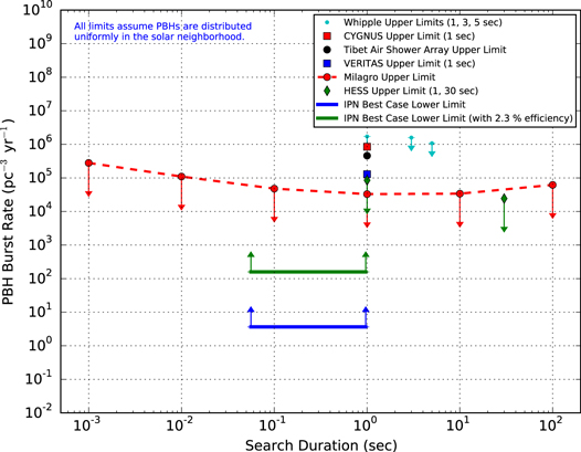
Figure 6. IPN PBH burst rate lower limit estimates assuming that all of the candidates are real PBH bursts. The horizontal green line gives the IPN PBH burst rate lower limit considering the selection efficiency of 2.3%. The blue horizontal line shows the lower limit if we assume 100% selection efficiency. Published PBH burst rate upper limits for various other burst search experiments are shown for comparison (Alexandreas et al. 1993; Amenomori et al. 1995; Linton et al. 2006; Tesic & VERITAS Collaboration 2012; Glicenstein et al. 2013; Abdo et al. 2015).
Download figure:
Standard image High-resolution imageIn the worst case scenario where none of our candidates are real PBH bursts, we cannot estimate a lower limit to the PBH burst rate density and instead consider estimating an upper limit to the PBH burst rate density. However, the assumption that none of the bursts in the sample is real but that we still have candidates implies that our criteria for identifying PBH bursts defined in Section 4 is not sufficient. This means that our method is not capable of setting an upper limit on the PBH burst rate density.
6. DISCUSSION
The detection of gamma-ray transients points to very high-energy explosive phenomena in the universe. Their detection in the solar neighborhood would indicate a previously unrecognized and potentially exotic phenomenon in our cosmic backyard. The sample of bursts identified in this paper consists of candidates for such explosions. They have short durations, no known afterglow detections, and distance limits consistent with the solar neighborhood. In principle, our methodology is capable of proving the local origin of bursts. However, in order to do so, we need either four widely separated, non-imaging spacecraft or two spacecraft that include one with imaging capability (see Section 3 and
First, it is of interest to investigate the sky distribution of our PBH burst candidates. For example, Cline et al. (1997) have argued that due to the fact that very short-duration GRBs (i.e., GRBs with duration ≤100 ms) have a non-isotropic sky distribution, they may be drawn from a different GRB population, possibly from PBH bursts. In order to investigate this, we have calculated burst density maps using the Gaussian kernel density methodology described in Ukwatta & Woźniak (2016). Since the sky locations of the PBH candidates depend on their distance from Earth, we started by assuming that all of the bursts are at their minimum distances and calculated their sky density map. This map is shown in Figure 7. The map is presented in Galactic coordinates with a 25° smoothing radius. It shows some relatively high-density areas, but the probability of generating this density contrast by chance, in the case when the true sky distribution is uniform, is ∼0.2, as estimated using a Monte Carlo simulation (Ukwatta & Woźniak 2016). Thus, the density structure seen in Figure 7 is consistent with a uniform source distribution. If these PBH candidates are real, then they cannot be further away than ∼10 pc (which is the maximum possible distance they can be detected assuming the optimistic Hagedorn-type model). We then also calculated the sky locations of the PBH candidates assuming they are at 10 pc and derived the sky density map as shown in Figure 8. This map is also consistent with a uniform source distribution. This is the behavior one would expect if these PBH burst are local with maximum detectable distance ∼10 pc.
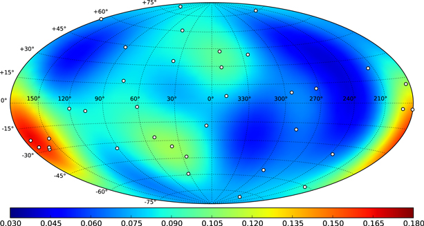
Figure 7. GRB density map in Galactic coordinates for the PBH burst candidates assuming the minimum distances given in Table 2. This map is normalized to represent a probability density function (PDF) that integrates to 1 over the entire sphere. The smoothing parameter is taken to be 25°. The circles indicate the locations of the individual bursts. The maximum and the minimum density values in this map are 0.166 and 0.041, respectively. The probability of generating this density contrast by chance in the case when the true sky distribution is uniform is ∼0.2 estimated using a Monte Carlo simulation (Ukwatta & Woźniak 2016). Thus, the density structures seen in the map are consistent with a uniform distribution.
Download figure:
Standard image High-resolution image
Figure 8. GRB density map in Galactic coordinates for the PBH burst candidates assuming constant distances of 10 pc to sources. The map has only 24 candidates with four spacecraft detections. Remaining eight bursts have only three spacecraft detections, so they do not have a single localization. This map is normalized to represent a probability density function (PDF) that integrates to 1 over the entire sphere. The smoothing parameter is taken to be 25°. The circles indicate the locations of the individual bursts. The maximum and the minimum density values in this map are 0.202 and 0.002, respectively. The probability of generating this density contrast by chance in the case when the true sky distribution is uniform is ∼0.1 estimated using a Monte Carlo simulation (Ukwatta & Woźniak 2016). Thus, the density structures seen in the map are consistent with a uniform distribution.
Download figure:
Standard image High-resolution imageAccording to the standard model for Hawking radiation (MacGibbon & Webber 1990), PBH bursts are standard candles, that is, all PBH bursts are intrinsically identical at the source. However, the way the burst appears at large distances may vary depending on its host environment. The final burst properties of the PBH burst depend on its mass and the number of fundamental particle degrees of freedom available at various energies (Ukwatta et al. 2016). In principle, by measuring the photon flux arriving from a PBH burst candidate in a given energy range, we can calculate the distance to that burst. However, during the last second of the PBH lifetime, its temperature is well above ∼1 TeV and the physics governing these high energies is not fully understood. Thus, the full spectrum of a PBH burst is difficult to calculate.
Ukwatta et al. (2016) have calculated PBH burst light curves in the 50 GeV–100 TeV energy range using the Standard Model of particle physics. This calculation considered both the direct Hawking radiation of photons from the black hole and the photons created due to the fragmentation and hadronization of the directly Hawking-radiated quarks and gluons. The expected PBH light curve is a power law with an index of ∼0.5, and at various sub-energy bands within the 50 GeV–100 TeV energy range has an interesting inflection point due to the brief dominance of the directly Hawking-radiated photons around ∼0.1 s before the PBH expiration. This is potentially a unique signature of a PBH burst in the GeV/TeV energy range.
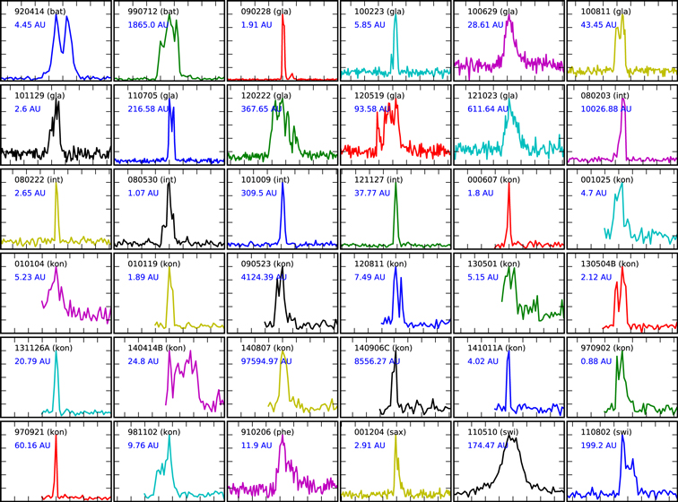
The detectors in the IPN are sensitive to photons in the energy range 10 keV–100 MeV. There are no published calculations of PBH burst light curves in the keV/MeV range using the Standard Model of particle physics to which we can fit our light curves and extract fit parameters. Nonetheless it is of interest to look at the light curves of our PBH burst candidates. First, we note that although a PBH will be emitting in the keV/MeV range before it becomes hot enough to emit in the GeV/TeV range, a keV/MeV burst signal can only be generated by the low-energy component of a PBH that is also emitting in the GeV/TeV range: this is because a 10 TeV black hole has a remaining burst lifetime of ∼1 s, whereas a <1 GeV black hole has a lifetime  and observationally would be a stable source, not a burst. This low-energy photon component, in turn, is predominantly generated by other higher-energy Hawking-radiated species via decays or the inner bremsstrahlung effect (Page et al. 2008) and is not the directly Hawking-radiated photon flux which decreases in the keV/MeV band as the burst progresses. Acknowledging the uncertainty in the PBH light curves in the keV/MeV range, it is also possible that the PBH burst signal may have a longer or shorter duration in the keV/MeV range than in the GeV/TeV range due to differences both in production at the source and in detector sensitivity, and that the duration difference varies with the distance to the PBH. Figure 9 shows the light curves of the 36 IPN bursts in our sample. Some are clearly single-peaked, others are clearly multi-peaked, and some were not recorded with sufficient statistics to determine the true number of peaks. It is interesting to note that bursts such as GRB 970921, GRB 080222, GRB 000607, GRB 101009, GRB 121127, GRB 131126A, and GRB 141011A display a keV/MeV time profile that resembles the PBH light curve profile calculated by Ukwatta et al. (2016) for the GeV/TeV energy range.
Figure 9. Normalized light curves of all the PBH burst candidates in the IPN sample. Black labels show the burst name with parenthesis showing the instrument. The blue labels give the minimum distance to the bursts based on our analysis. Each light curve shows a time range of 4 s centered on the brightest peak.
Download figure:
Standard image High-resolution image
In this paper, we introduced a novel method to constrain the distances to GRBs using detections from multiple spacecraft. Utilizing detections from three non-imaging spacecraft, we could only constrain the minimum distances to our current sample of bursts. The maximum distance is constrained by the energy available during the final second of the PBH burst. However, the amount of energy released in the keV/MeV energy band is not known and may be highly model-dependent. On the other hand, with detections by four widely separated (∼au distances), non-imaging spacecraft, or one non-imaging spacecraft and one imaging spacecraft, we can constrain burst distances independent of any high-energy physics model, and potentially show that some bursts are local. Such a detection will not only prove the existence of PBH bursts, by fitting light curves and spectra derived using various beyond the standard model physics theories, we can also identify which theory describes nature.
Support for the IPN was provided by NASA grants NNX09AU03G, NNX10AU34G, NNX11AP96G, and NNX13AP09G (Fermi); NNG04GM50G, NNG06GE69G, NNX07AQ22G, NNX08AC90G, NNX08AX95G, and NNX09AR28G (INTEGRAL); NNX08AN23G, NNX09AO97G, and NNX12AD68G (Swift); NNX06AI36G, NNX08AB84G, NNX08AZ85G, NNX09AV61G, and NNX10AR12G (Suzaku); NNX07AR71G (MESSENGER); NAG5-3500, and JPL Contracts 1282043 and Y503559 (Odyssey); NNX12AE41G, NNX13AI54G, and NNX15AE60G (ADA); NNX07AH52G (Konus); NAG5-13080 (RHESSI); NAG5-7766, NAG5-9126, and NAG5-10710, (BeppoSAX); and NNG06GI89G. T.N.U. acknowledges support from the Laboratory Directed Research and Development program at the Los Alamos National Laboratory (LANL). The Konus-Wind experiment is partially supported by a Russian Space Agency contract and RFBR grants 15-02-00532 and 13-02-12017-ofi-m. We also thank Jim Linnemann (MSU), Dan Stump (MSU), Brenda Dingus (LANL), and Pat Harding (LANL) for useful conversations on the analysis.
APPENDIX: GRB TRIANGULATION WHEN THE SOURCE DISTANCE IS ALLOWED TO VARY
Assume that two spacecraft,  and
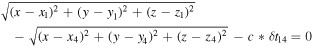
and  , separated by a distance d, observe a GRB. For any assumed distance between the GRB and the spacecraft, the difference in arrival times δt12 must be constant. Let x1, y1, z1 and x2, y2, z2 be the coordinates of the two spacecraft. Then, the locus of points x, y, z which describes the possible source locations is given by
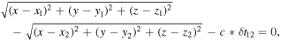
where c is the speed of light.
First, for simplicity, consider the two-dimensional problem. Let  and
and  define the z-axis of a coordinate system whose origin is halfway between the spacecraft. The positions of
  and
and  are the foci of the hyperbola:
This is shown in Figure 1. Here,  is the difference between the distances of any point on the hyperbola from the foci, so
  and
and  . For every point on this hyperbola, the difference in the arrival times is
  . If we assume an infinite distance for the source, then the asymptotes of the hyperbola define the two possible arrival directions of the GRB.
Now consider the three-dimensional case. If we rotate the hyperbola of Figure 1 about the z-axis, then we obtain one sheet of a hyperboloid of rotation of two sheets. Its formula is

Here, the x-axis is perpendicular to the y- and z-axes, and cuts in the plane z = constant give circles. This is illustrated in Figure 2.
In practice, we will have two or more hyperboloids generated by three or more spacecraft, and we will want to work in Earth-centered Cartesian coordinates with one axis oriented toward R.A. zero, decl. zero, and another axis oriented toward decl. 90°. Consider the three-spacecraft case. A spacecraft pair will define two foci of a hyperboloid; the line joining the two spacecraft, which defines the axis of rotation of the hyperboloid, will be oriented with respect to Earth-centered coordinates such that it represents a rotation and a translation. We want to express the formula for the hyperboloid in the Earth-centered system.
The coordinate rotation can be described by three sets of direction cosines:
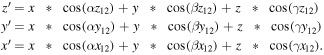
Here, the primed coordinate system is the one defined by the foci of the hyperboloid; its origin is the same as that of the unprimed, Earth-centered system, and it is rotated, but not translated, with respect to it. Now, we perform a translation of the primed system so that its origin is at the midpoint of the two foci. If the coordinates of the two spacecraft, expressed in the unprimed system, are x1, y1, z1 and x2, y2, z2, then the origin of the translated system will be at (x1 + x2)/2, (y1 + y2)/2, (z1 + z2)/2. The formula for the hyperboloid, expressed in the Earth-centered system, becomes
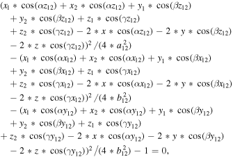
where a12 and b12 refer to the hyperboloid for spacecraft 1 and 2. A similar equation describes the hyperboloid for spacecraft 1 and 3. Although a third equation can be derived for spacecraft 2 and 3, it is not independent of the other two because it is constrained by the condition  + δ t13 + δ t32 = 0.
The locus of points describing the intersection of two hyperboloids is a simple hyperbola contained in a plane. This is shown in Figure 3. This hyperbola contains all of the points satisfying the time delays for the two spacecraft pairs, δ t12 and δ t13, when the GRB distance is allowed to vary. The two branches of the hyperbola intersect the celestial sphere at two points; if the distance is taken to be infinite, then the two points are the possible source locations. It follows that a GRB observed by three, and only three, widely separated, non-imaging spacecraft cannot be unambiguously proven to originate at a local distance; on the other hand, in the case where the hyperbola degenerates to a single point, that point must be at an infinite distance and a local origin can be ruled out. None of the bursts in this sample were in this category.
In the simplest case, we have one spacecraft near Earth and two spacecraft in interplanetary space. So
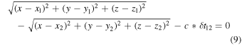
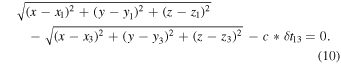
The lower limit to the source distance is the point on the hyperbola (x, y, z) which is closest to Earth. This can be found by solving for the minimum of the expression  (the Earth distance) subject to the constraints imposed by Equations (9) and (10). In practice, there are uncertainties associated with δt12 and δt13, and we have used the most probable values to derive the lower limits. Since x, y, and z vary along the hyperbola, the apparent arrival direction for an observer at Earth depends on the assumed distance; if the source distance is assumed to be infinite, then the derived R.A. and decl. will not be correct if the source is actually local. For example, if GRB 140807 were at its minimum allowable distance (1.46 × 1018 cm, or 9.8 × 10⁴ au), then the angle between its true coordinates and the coordinates for an infinitely distant source would be 0
 04. However, for GRB 101129, whose minimum allowable distance is only 3.89 × 1013 cm, or 2.6 au, the angle would be 542.
In a number of cases, a fourth non-coplanar experiment, in this case Konus-Wind, at up to 7 light-seconds from Earth, can be used to constrain the lower limits further. Adding the constraint
eliminates one branch of the hyperbola and part of the second branch, leading to a larger distance lower limit. Thus, in the case of four widely separated spacecraft, it is in principle possible to rule out an infinite distance and prove that the origin is local, as illustrated in Figure 4. However, this was not the case for any of the bursts in this study; they are all consistent with both local and infinite distances.
Note that this method does not depend on the properties of the GRB itself, such as duration or intensity; the lower limit is determined by the IPN configuration (through the spacecraft coordinates) and the direction of the burst (through the time delays). Thus, for example, it can be applied equally to long- and short-duration bursts, and a sample of long-duration events would yield a distribution of lower limits which was comparable to a sample of short-duration events.
One special case should be noted here. With just two widely separated spacecraft, if one has precise imaging capability, then the problem reduces to finding the intersection of a hyperboloid and the vector defined by the precise localization from the imager. In principle, a local origin can be demonstrated or a distance lower limit can be obtained. We have studied approximately 200 GRBs in this category, and analysis of the results is ongoing.