


ABSTRACT
We use a method developed by Roberts that optimizes the phase angles of an ensemble of plane waves with amplitudes determined from a Kolmogorov-like power spectrum, to construct magnetic field vector fluctuations having nearly constant magnitude and large variances in its components. This is a representation of the turbulent magnetic field consistent with that observed in the solar wind. Charged-particle pitch-angle diffusion coefficients are determined by integrating the equations of motion for a large number of charged particles moving under the influence of forces from our predefined magnetic field. We tested different cases by varying the kinetic energy of the particles (Ep) and the turbulent magnetic field variance ( ). For each combination of Ep and
  , we tested three different models: (1) the so-called "slab" model, where the turbulent magnetic field depends on only one spatial coordinate and has significant fluctuations in its magnitude (
 ); (2) the slab model optimized with nearly constant magnitude b; and (3) the slab model turbulent magnetic field with nearly constant magnitude plus a "variance-conserving" adjustment. In the last case, this model attempts to conserve the variance of the turbulent components (
 ), which is found to decrease during the optimization with nearly constant magnitude. We found that there is little or no effect on the pitch-angle diffusion coefficient
  between models 1 and 2. However, the result from model 3 is significantly different. We also introduce a new method to accurately determine the pitch-angle diffusion coefficients as a function of μ.
Export citation and abstract BibTeX RIS
1. INTRODUCTION
The transport of high-energy charged particles in the heliosphere, including galactic cosmic rays and solar-energetic particles, is known to be affected significantly by the random or turbulent component of the interplanetary magnetic field embedded in the solar wind. The distribution of these particles in space, time, and energy is governed by the cosmic-ray transport equation (Parker 1965), which requires transport coefficients that depend on solar wind turbulence. The study of the turbulent interplanetary magnetic field is an active area of research (Dobrowolny et al. 1980; Matthaeus et al. 1990; Tu & Marsch 1993; Dasso et al. 2005; Podesta et al. 2007; Horbury et al. 2008), and there are a number of different models that have been discussed (Tu & Marsch 1993; Bieber et al. 1996; Boldyrev 2006; Horbury et al. 2008). It is important to understand how transport coefficients computed from the motion of particles depend on these different turbulence models. Besides theoretical completeness, this study is also applicable to the prediction of energetic particle intensities during increased solar wind activity and is also relevant to the propagation of cosmic rays in the galactic magnetic field.
Observations show that the variance of the magnitude of the magnetic field in solar wind turbulence is much smaller than the variance of its components (Belcher & Davis 1971; Roberts 2012). This feature of the solar wind turbulence has not been previously considered when deriving transport coefficients of charged-particle transport in magnetic turbulence (Jokipii 1966; Matthaeus et al. 2003). Previous numerical calculations (Giacalone & Jokipii 1999) were only concerned with the turbulence models such as isotropic, composite (Matthaeus et al. 1990; Tu & Marsch 1993; Bieber et al. 1996), and anisotropic (Goldreich & Sridhar 1995) magnetic turbulence. None of these models minimize the variance of the magnitude of the magnetic field. In this study, we adopt a new method, proposed by Roberts (2012), to synthesize magnetic turbulence with nearly constant magnitude and calculate the diffusion coefficients of charged particles in this field.
2. MAGNETIC FIELD MODEL
We consider a magnetic field of the form  , where
  is the mean field and
  is a zero-mean random field. In order to produce a field with nearly constant fluctuation in magnitude, we follow the procedure described by Roberts (2012). For simplicity, but without loss of generality, we assume that the random part of the turbulent magnetic field,
  , is given by


where  represents the amplitude of the fluctuation, kn is the wavenumber along the z-axis,
  and
and  are the phase angles of these two linear modes, and b(z) is the magnitude of the magnetic field at any given point of interest. Note that
  . We also note that b(z) only depends on z, the direction of the average magnetic field. Because this is a one-dimensional turbulent magnetic field, there are two ignorable coordinates, and it follows that charged particles must remain within one gyroradius of the magnetic line of force in which it starts its motion (Jokipii et al. 1993). In this paper we are concerned only with pitch-angle diffusion.
The amplitudes in the sums given in Equations (1) and (2) are determined from a one-dimensional Kolmogorov spectrum given by


where C is a normalization constant and LC is the correlation length of the magnetic fluctuations. The normalization is such that the total variance is  .
.
According to Roberts (2012), the phase angles  and
and  are chosen such that the variance
  is a minimum. This is called an "optimization." In practice, one needs to define the "sampling" points, which are a set of points,
  . They will be used to evaluate
  , the variance of b(z) in Equation (3) during the optimization. As a result of the optimization, we also find that the variance of the Bx and By components (
 and
and  ) of the magnetic field also decreases as in Figure 1. This is because the chosen sampling points do not cover a large enough range in z to maintain the variance of the Bx and By components of the magnetic fields. To clarify this point, consider a simpler case of just two wave modes, such that

The variance is given by  , and T is the range of the sampling points in z. Then we have
The first and second terms will average to 1/2 given a large enough integration range in z, say,  . The third and the fourth terms will only average to zero given that the integration range in z is as large as
  .
.

Figure 1. Magnetic field before the optimization and after the optimization along z. The red line is the x component and the blue line is the y component of the magnetic field along z. The black line is the magnitude of the magnetic field along z. LC is the correlation length of the magnetic fluctuations, and B0 is the magnitude of the mean magnetic field.
Download figure:
Standard image High-resolution imageIn our more general case, the range of z that is used in the optimization is  . The smallest space between two points in the set of sampling points used for the optimization is
  . This is a compromise between the optimization and the computational efficiency. However, this range in z is not large enough to make all the cross-terms, such as the third and fourth terms in the simple example given above, average to zero, as expected mathematically. Nevertheless, the optimization still leads to smaller magnitude fluctuations and relatively large fluctuations in the components of
  as long as both the range of z and number of sampling points are sufficiently large.
Figure 2 demonstrates this effect. We use a new factor,  , to indicate the difference of the total variance of the fluctuating part
  and
and  before and after the optimization. This gives

Here the subscript "before" means before the optimization, and "after" means after the optimization. In Figure 2 these two plots are from two sets of optimization runs. The top panel shows the effect of optimizing the field with a fixed range of z while using various numbers of sampling points (or sampling interval). It shows that we need to choose a large enough number of sampling points to minimize the scale-up effect. However, there is a turnover point that suggests that the scale-up effect will not disappear as we further increase the number of sampling points. The bottom panel describes the effect of increasing the range of z while fixing the sampling interval. In this case, the scale-up factor approaches unity as we increase the range of z while keeping a large enough number of sampling points in the optimization.
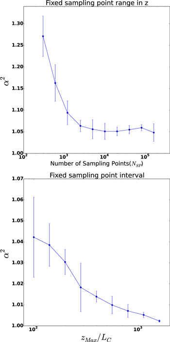
Figure 2. Numerical experiments that test the dependence of  in Equation (6) on the number of sampling points (top panel, with fixed sampling point range in z) and the sampling point range in z (bottom panel, with fixed sampling point interval). Each data point has its mean as the solid dot and its standard deviation as the error bar. Recall that the sampling points are used to calculate the variance of the field magnitude during the optimization. In the top panel, all the test runs have the same range in z as
  . In the bottom panel, all the test runs have the same sampling interval as
  .
.
Download figure:
Standard image High-resolution imageMoreover, we can compensate for this effect by multiplying both amplitudes of the Bx and By components by the new factor as in Equation (6), α, to raise the total variance back to the same level as before the optimization. We refer to this procedure as "scale-up" in the numerical experiment. We perform simulations both using this scale-up procedure and without it to study its effect on our results.
To set up the magnetic field described by Equations (1)–(5), we use a maximum wavelength  and a minimum wavelength
  for the linear modes. We use 20,000 points along the z-axis over the range of
 ![$[-50{L}_{C},50{L}_{C}]$](https://content.cld.iop.org/journals/0004-637X/827/1/16/revision1/apjaa2b18ieqn36.gif) . The correlation length is taken to be 0.01 au as observed in the near-Earth solar wind (Matthaeus & Goldstein 1982; Matthaeus et al. 2005; Wicks et al. 2009, 2010). For the magnetic fluctuations, we fix the mean field at 5 nT with the standard deviation chosen at
. The correlation length is taken to be 0.01 au as observed in the near-Earth solar wind (Matthaeus & Goldstein 1982; Matthaeus et al. 2005; Wicks et al. 2009, 2010). For the magnetic fluctuations, we fix the mean field at 5 nT with the standard deviation chosen at  = 1, 0.09, and 0.01. This set of values represents the strong turbulence, mild turbulence, and weak turbulence in the solar wind magnetic field, respectively. The weak turbulence case could also be used to check the numerical result with the standard quasi-linear theory (QLT). We have simulated five different combinations of particle energies and variances of the magnetic field strength (see the next section). For each combination, we tested three situations: (1) without optimizations, (2) with optimizations, and (3) with optimizations and the scale-up procedure (described above). These are listed in Table 1. We note that in each case, the mean-free path of the particles is much less than the box size.
Table 1. Simulation Parameters for All the Numerical Experiments
| Simulation Parameters | ||||||||||
|---|---|---|---|---|---|---|---|---|---|---|
| Case | Energy |

|
Nm | Nc | Np | Rw | Nb |

|
Optimize | Scale-up |
| (GeV) | 1 | 1 | 20000 | 1 | 1 | 2000 |

|
Flag | Flag | |
| 1 | 10 | 0.09 | 200 | 1 | 400 | 0.05 | 1 | 0.001 | Off | Off |
| 2 | 1 | 1 | 200 | 1 | 400 | 0.05 | 1 | 0.001 | Off | Off |
| 3 | 1 | 0.09 | 200 | 1 | 400 | 0.05 | 1 | 0.001 | Off | Off |
| 4 | 1 | 0.01 | 200 | 1 | 400 | 0.05 | 1 | 0.001 | Off | Off |
| 5 | 0.1 | 0.09 | 200 | 1 | 400 | 0.05 | 1 | 0.001 | Off | Off |
| 6 | 10 | 0.09 | 200 | 1 | 400 | 0.05 | 1 | 0.001 | On | Off |
| 7 | 1 | 1 | 200 | 1 | 400 | 0.05 | 1 | 0.001 | On | Off |
| 8 | 1 | 0.09 | 200 | 1 | 400 | 0.05 | 1 | 0.001 | On | Off |
| 9 | 1 | 0.01 | 200 | 1 | 400 | 0.05 | 1 | 0.001 | On | Off |
| 10 | 0.1 | 0.09 | 200 | 1 | 400 | 0.05 | 1 | 0.001 | On | Off |
| 11 | 10 | 0.09 | 200 | 1 | 400 | 0.05 | 1 | 0.001 | On | On |
| 12 | 1 | 1 | 200 | 1 | 400 | 0.05 | 1 | 0.001 | On | On |
| 13 | 1 | 0.09 | 200 | 1 | 400 | 0.05 | 1 | 0.001 | On | On |
| 14 | 1 | 0.01 | 200 | 1 | 400 | 0.05 | 1 | 0.001 | On | On |
| 15 | 0.1 | 0.09 | 200 | 1 | 400 | 0.05 | 1 | 0.001 | On | On |
Note. Nm is the number of wave modes in both  and
and  . Nc is the number of sampling points. Np is the number of test particles. Rw is the radius of the sliding window for the numerical experiment for calculating the
  . Nb is the number of bins in the μ space ([−1, 1]) used to calculate
  .
.
Download table as: ASCIITypeset image
3. TRACKING THE ENERGETIC CHARGED PARTICLES
A charged particle moving in a magnetic field, such as that described in the previous section, will move according to the Lorentz force equation given by

where q is the charge,  the Lorentz factor, m the mass,
  the velocity, and c the speed of light. We solve this set of equations by using the eighth-order adaptive step-size Runge–Kutta method to update the particle's velocity and position at each time step (Hairer et al. 1993). We record the particle's motion at the step size of
  to resolve the short enough timescale required for scattering calculations. For the highest-energy particles (
 ), the energy is well conserved by this very high order numerical integration method up to at least
  in our test, which is longer than all the cases in our simulations. We choose three energies for the charged particles for calculations: 10 GeV, 1 GeV, and 100 MeV. Thus, our approach is also suitable for cosmic-ray transport in the interstellar medium.
4. DETERMINING THE PITCH-ANGLE DIFFUSION COEFFICIENT, 

In order to determine  , the pitch-angle diffusion coefficient, we use a method similar to that proposed by Kaiser et al. (1978). The approach is based on the numerical integration of motion of a very large number of test particles in the synthetic magnetic field described in the previous section. It is assumed that the collection of the particles, described by a distribution function, f, obeys the pitch-angle diffusion equation given by

where μ is the cosine of the pitch angle,  is the diffusion coefficient, and
  is in general the source function to be supplied. The steady-state solution to Equation (8) for absorbing boundary conditions,
  , where
  is the region of the solution, and a point source of the particles at
  of the form
  , where
  is the injection μ, is given by (Kaiser et al. 1978)

where JL and JR are the flux of particles crossing the left and right boundaries  and
and  , respectively.
Because of the  factor in the denominator of Equation (9), this process leads to a rather "noisy" or uncertain determination of
  . To reduce the noise, and aiming at a more accurate calculation of f, we use a "sliding-window" approach, where the entire μ range from −1 to 1 is subdivided into 2000 smaller regions that overlap one another. This is illustrated in Figure 3.
  is determined in each smaller region and averaged at each bin over all the sliding windows given by

where  is the number of sliding-window values that the ith bin accumulates during the experiment. This gives a much smoother and statistically significant
  . For each bin 400 particles are used to determine
  from Equation (9). We count how many (NL) particles leave from the left boundary in μ and how many (NR) leave from the right boundary in μ in each bin, and then we have


where  is one time step in the simulation. We also have that for the ith bin in μ space,

We apply a linear regression on  over μ to calculate
  . By fitting to the above solution in f, μ, and J, we have an estimate of the scattering coefficients over the one sliding window of
 ![$[{\mu }_{L},{\mu }_{R}]$](https://content.cld.iop.org/journals/0004-637X/827/1/16/revision1/apjaa2b18ieqn70.gif) in the μ space. The width of each sliding window is 0.05, and the bin size (to compute
in the μ space. The width of each sliding window is 0.05, and the bin size (to compute  within each window) in the μ space is 0.001. We slide the window through [−1, 1] to cover the whole μ space, with a sliding distance of 0.009 in the μ space until out of its range. This procedure gives
  as a function of the entire region of μ from −1 to 1. Note that for each window, we use 400 particles per realization and 48 realizations, for a total of 400 × 48 particles.

Figure 3. Schematic plot of sliding windows used in the numerical experiments for calculating the scattering coefficients. The unit in the y-axis is arbitrary. Each sliding window (e.g., the  window ) has a left boundary (
 ) and a right boundary (
 ). We calculate the scattering coefficients
  for each window, and by sliding the windows through the μ space, we have an estimate of the
  over the range of μ. The window has to be wide enough for the diffusion process described in Equation (8).
Download figure:
Standard image High-resolution image5. RESULTS
Table 1 summarizes the 15 total simulations performed in this study. Figures 4 and 5 show our calculation of the pitch-angle diffusion coefficient  versus μ for all of these simulations. In each figure, the prediction from QLT is also plotted as a series of plus signs. Notice that when the magnetic field is strongly turbulent (high variance), there is a significant departure from the QLT prediction, but when the field is weakly turbulent (low variance), the simulation results are closer to the QLT prediction.

Figure 4.
 calculated for particles with different energies with and without field optimizations. (top) Cases 1, 6, and 11 in Table 1; (middle) cases 3, 8, and 13 in Table 1; (bottom) cases 5, 10, and 15 in Table 1. "OPT OFF" means that there is no optimization, and the data are marked as solid lines. "OPT 1 ON" means that optimization is applied, but without scale-up procedures. The data in this case are marked as dashed lines. "OPT 2 ON" means that both optimization and scale-up are applied to the fields. "QLT" means the quasi-linear theory estimates. The data in this final case are marked as dotted lines.
Download figure:
Standard image High-resolution imageFigure 4 shows how  varies for different particle energies but with the magnetic turbulence variance fixed. For each energy, we tested three situations: (1) the normal slab turbulence, (2) the normal slab turbulent magnetic field with the nearly constant magnitude ("optimize flags" on), and (3) the normal slab turbulent magnetic field with the nearly constant magnitude plus the variance-conserving adjustment ("scale-up flags" on). These are represented with different curves of different colors as indicated in the figure. In each of the energies shown we find that there is little difference between the situations without any optimization and situations with only optimizations (no difference between blue and red colors). Thus, we find that by reducing the fluctuations in the magnitude there is essentially no effect on
  . We note that while the magnitude of the field has been optimized to have little variation, the components also have less variation compared to the no-optimization case. Thus, it seems that even though the magnitude is nearly constant, the reduction in the variance in the components leads to there being no effect on
  . On the other hand, we note that there is a significant increase in
  relative to the no-optimization case, if we apply the "scale-up" procedure. The increase in
  in this case likely is the result of the slight increase in the variance of the components resulting from the scale-up procedure (see Section 2).
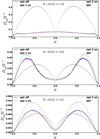
Figure 5 shows the results for three different values of the turbulence variance ( , 0.09, 0.01 from top to bottom) but with the particle energy fixed (
 ). As we did for Figure 4, we tested three separate cases. The most striking result is that when the variance is large, as in the top panel, there is a significant departure form the QLT prediction, and the largest value of
  occurs at
  . This is generally consistent with the result reported by Kaiser et al. (1978). We also note that an enhancement in
  at
at  was discussed by Jones et al. (1978), who interpreted this as the result of magnetic mirroring. However, in our case, the optimization is intended to reduce the fluctuations in the magnitude of the magnetic field, which would reduce the magnetic mirroring. At present, we do not fully understand this. On the other hand, one finds in the bottom panel that QLT gives much better predictions over μ when the variance is very low and the assumption of the QLT is guaranteed.
Figure 5.
 calculated for particles with different energies with and without field optimizations. (top) Cases 2, 7, and 12 in Table 1; (middle) cases 3, 8, and 13 in Table 1; (bottom) cases 4, 9, and 14 in Table 1. "OPT OFF" means that there is no optimization, and the data are marked as solid lines. "OPT 1 ON" means that optimization is applied, but without scale-up procedures. The data in this case are marked as dashed lines. "OPT 2 ON" means that both optimization and scale-up are applied to the fields. "QLT" means the quasi-linear theory estimates. The data in this final case are marked as dotted lines.
Download figure:
Standard image High-resolution image
One possible reason that the optimization has no effect on the scattering might be because the optimization is highly related to the sampling points. The sampling points are those positions along z that are chosen and used to calculate the variances of the magnetic field magnitude and its components ( ,
,  ,
,  ) and perform the optimization. In our simulation, we chose 20,000 points in the range
 ![$[-50{L}_{C},50{L}_{C}]$](https://content.cld.iop.org/journals/0004-637X/827/1/16/revision1/apjaa2b18ieqn95.gif) along the z-axis, which means that the smallest resolvable wavelength in our sampling point set is
along the z-axis, which means that the smallest resolvable wavelength in our sampling point set is  . This happens to be the shortest wavelength of the linear modes we used to generate the magnetic fluctuations and hence should be enough for the purpose of the optimization. However, we note that the minimization is valid in the sampling points we chose to perform the optimization. For the purpose of performing the subsequent diffusion calculations, we should have included all the positions along z that each particle might have visited. However, when we perform test particle simulations, the high-precision particle tracker algorithm will advance in such a tiny time step (
 ) that the spatial advancement of a particle (
 ) might be much smaller than the smallest wavelength of the linear modes (
 ), which is also the sampling interval of the sampling points used for the optimization. Therefore, the result is as if the test particle simulation is advancing on a dense and compact mesh while the optimization is performed on a relatively loose and sparse one. Thus, the effect of the optimization might not be significant enough. However, due to the nonlinearity of the scattering system, it is only possible to make the mesh grid of the sampling points used for the optimization approach the density and compactness of the set of the positions many particles would travel in the same region, which has infinite points theoretically. This also explains the difficulty in practice to extend the same algorithm to the higher-dimension magnetic turbulence models. Nevertheless, in our experiments, there is no significant effect observed on the scattering from the optimization.
Another interesting result is the effect of the scale-up procedures. In all cases, it shows a significant increase in the scattering. This again is related to the fact that we could only use a limited number of sampling points. Therefore, although applying the scale-up procedure will not change the variance of the turbulent field over the same set of sampling points, the actual variance is increased if we include all the possible points in the range ![$[-50{L}_{C},50{L}_{C}]$](https://content.cld.iop.org/journals/0004-637X/827/1/16/revision1/apjaa2b18ieqn100.gif) along the z-axis when calculating the variance. According to the QLT (Jokipii 1966), it is apparent that the scattering would be enhanced in more turbulent fields while keeping other conditions the same. Therefore, one should not include the scale-up procedure in the optimization in the future numerical experiments.
along the z-axis when calculating the variance. According to the QLT (Jokipii 1966), it is apparent that the scattering would be enhanced in more turbulent fields while keeping other conditions the same. Therefore, one should not include the scale-up procedure in the optimization in the future numerical experiments.
It should be noticed that through our numerical simulations we thought about the possible effect of different optimization algorithms. Mathematically, one could choose a brute-force method or some other method, such as the gradient descent method or stochastic gradient descent method (both are commonly used in searching for the maximum/minimum of the nonlinear multivariable functions), to find the optimized set of  and
and  to minimize the variance of the magnitude of the magnetic field. In this case, the latter ones have the merit of computational efficiency and convenience of coding in practice. However, the brute-force method is very reliable in searching for the global minimum, while the more advanced methods might stop the search at a local minimum, which is hard to diagnose.
6. CONCLUSION
In this paper we numerically integrated the equation of motion for a large number of charged particles moving in a kinematically prescribed turbulent magnetic field optimized so as to reduce the level of fluctuations in the magnitude of the field. We computed the pitch-angle diffusion coefficient as a function of μ by assuming that the pitch-angle distribution can be described by the well-known pitch-angle diffusion equation. We used a new "sliding-window" method, which is an improvement on previous approaches to obtain a smooth, statistically significant representation of  versus μ. We tested results for different combinations of the charged-particle energies and the turbulent magnetic field strengths. For each combination, we tested three different models: (1) the so-called "slab" model, in which the turbulent magnetic field depends on only one spatial coordinate and has significant fluctuations in its magnitude (
 ); (2) the slab model optimized with nearly constant magnitude b; and (3) the slab model turbulent magnetic field with nearly constant magnitude plus a "variance-conserving" adjustment (see Section 2 for details).
We found that there is no effect on particles' scattering over the pitch-angle space by only applying the optimization to the turbulent magnetic fields. We did find, however, that there is an increase in  when we apply the variance-conserving adjustment after the optimization (see Section 2 for details). This is due to our observation that the optimization will result in a decrease in the variances of both
  and
and  when we minimize the variance of the field magnitude
  . We therefore compensate the decrease in
  and
and  by multiplying by a factor of
  as in Equation (6) to conserve the total energy of the fluctuation.
We note that the phase angles in Fourier components of  and
and  for each wavenumber k are assumed to be random in the beginning, but are not so after the optimization, as pointed out in Roberts (2012). This might have significant influence on the decrease in
  and
and  during the optimization.
We have also found that our new method of calculating the  versus μ by applying the "sliding-window" approach to the procedure initially proposed by Kaiser et al. (1978) is an efficient numerical method to determine charged-particle scattering in the turbulent magnetic fields, which will lead to a smooth and statistically significant result of
  versus μ.
Since we only considered a one-dimensional field model in this study, future work could use this optimization in the three-dimensional isotropic turbulent magnetic field models while performing the numerical experiment on the diffusion in both the μ-space and the real space for charged particles to observe the effects of the optimizations. This could be important for determining the cross-field diffusion, discussed, for example, in Giacalone & Jokipii (1999).
We acknowledge helpful discussions with D. Aaron Roberts, Jozsef Kota, and Federico Fraschetti. This work was supported in part by NASA under grants NNX15AJ72G and NNX15AJ71G.