


ABSTRACT
We report observations of low-frequency waves at 1 au by the magnetic field instrument on the Advanced Composition Explorer (ACE/MAG) and show evidence that they arise due to newborn interstellar pickup He+. Twenty-five events are studied. They possess the generally predicted attributes: spacecraft-frame frequencies slightly greater than the He+ cyclotron frequency, left-hand polarization in the spacecraft frame, and transverse fluctuations with minimum variance directions that are quasi-parallel to the mean magnetic field. Their occurrence spans the first 18 years of ACE operations, with no more than 3 such observations in any given year. Thus, the events are relatively rare. As with past observations by the Ulysses and Voyager spacecraft, we argue that the waves are seen only when the background turbulence is sufficiently weak as to allow for the slow accumulation of wave energy over many hours.
Export citation and abstract BibTeX RIS
1. INTRODUCTION
For the purposes of this paper, the interstellar medium is composed primarily of ions, electrons, a magnetic field, and neutral atoms. The charged particles and magnetic field form a plasma that interacts with the solar wind and heliospheric magnetic field (HMF) to form a termination shock, heliosheath, and perhaps a bow shock surrounding the heliosphere (McComas et al. 2012). Neutral atoms pass through this region and the solar wind without interaction until they are ionized mainly by either charge exchange with solar wind ions or photoionization by solar EUV flux (Blum & Fahr 1970; Axford 1972; Holzer 1972; Vasyliunas & Siscoe 1976; Möbius et al. 1985; Gloeckler et al. 1993; Geiss et al. 1994). For some species, electron impact ionization may also be important. Once ionized they form a "pickup" population and the newborn ions gyrate around the HMF with their energy determined by the solar wind speed relative to their drift speed through the heliosphere and their pitch angle determined by the magnetic field orientation at the point of ionization. Hydrogen (H) is the dominant neutral atom followed by helium (He). Neutral atoms approach Earth from a direction given by the motion of the heliosphere through the local interstellar medium. Hydrogen is ionized primarily by a combination of charge exchange and photoionization. Ionization of hydrogen is so efficient that the neutral atom density falls exponentially at 4–5 au, forming an ionization cavity in the inner solar system. Helium ionization is primarily by photoionization and is less efficient (Bzowski et al. 2012, 2013a, 2013b). To leading order, neutral He density is almost constant in the upwind direction and forms a gravitational focusing cone of enhanced density behind the Sun that the Earth passes through in December. Zank (1999) and McComas et al. (2015a, 2015b) provide excellent reviews of these conditions.
Newborn interstellar pickup ions (PUIs) form gyrating beams. These ion beams develop kinetic instabilities that have also been studied extensively in the context of planetary, interplanetary, and cometary foreshocks (Barnes 1970; Gary et al. 1984; Glassmeier et al. 1989; Johnstone et al. 1991; Gray et al. 1996). In the examples shown here, the HMF is nearly radial and the initial pitch angle ≃0°. Resonant beam instabilities are then the dominant means of wave energy excitation by newborn interstellar PUIs. Under these radial field conditions, quasilinear theory describes the generation of transverse, noncompressive waves propagating sunward and parallel to the mean magnetic field (Wu & Davidson 1972; Lee & Ip 1987; Isenberg 1996). The ionization rate for new interstellar PUIs is small, so the instability is weak and the accumulation of wave energy is slow.
Although the early theoretical work suggests that the low-frequency waves associated with the scattering of newborn interstellar PUIs should be a ubiquitous feature of the interplanetary spectrum, they are actually relatively rare and difficult to find. Murphy et al. (1995) reported 31 examples of low-frequency waves associated with newborn pickup H+ that were recorded by the Ulysses spacecraft. Joyce et al. (2010) reported one event in the Voyager 2 data at 4.5 au where waves were excited by both newborn interstellar H+ and He+. Smith et al. (2010) and Cannon et al. (2013, 2014a) revisited the Ulysses data using daily spectrograms to search for additional wave events and found 502 intervals of waves excited by newborn pickup H+.
The energy of excited waves is subject to the background turbulence, which couples to the waves and disperses the wave energy. The wave energy is transported via turbulent processes to small scales where dissipation converts the turbulent fluctuations into heat. The addition of wave energy associated with the scattering of newborn interstellar PUIs has been shown to provide a critical component that is necessary to explain solar wind heating in the outer heliosphere (Zhou & Matthaeus 1990a, 1990b; Matthaeus et al. 1994; Richardson et al. 1995, 1996; Zank et al. 1996, 2012; Smith et al. 2001, 2006a; Isenberg et al. 2003, 2010; Richardson & Smith 2003; Breech et al. 2005, 2008, 2009, 2010; Isenberg 2005; Ng et al. 2010; Oughton et al. 2011).
Our more recent analyses have shown that turbulence is a major factor in determining the observability of the waves. Waves are observed when the background turbulence is weaker than the instability driving the waves (Cannon et al. 2014b). Following this insight, Aggarwal et al. (2016) re-examined Voyager magnetic field data looking for times when the turbulence would be weak and found 11 additional examples of waves due to newborn interstellar PUIs. Some of those waves arise from He+ and some from H+.
In a demonstration of the techniques used here, Argall et al. (2015) employed daily spectrograms to search magnetic field data from the Advanced Composition Explorer (ACE) spacecraft and reported one example of waves excited by newborn interstellar pickup He+. In this paper we continue the analysis of Argall et al. (2015) and perform a statistical analysis of 25 wave events found in the ACE magnetic field data from day 23 of 1998 to day 209 of 2015. We perform a spectral analysis of the events including power spectra of each component in mean-field coordinates, magnetic helicity, and polarization parameters. We then compute instability rates using observed solar wind parameters and theoretical expressions for interstellar neutral (ISN) He densities and ionization efficiency. These instability rates are then compared to the rate of turbulent cascade, where we again find that the observability of the waves is based on the background turbulence being weak when compared to nominal solar wind conditions at 1 au.
2. THEORY
The waves reported here originate with ISN He atoms that freely penetrate the heliosphere until photoionization liberates an electron and these new ions form a pickup population of suprathermal particles. As the ions scatter, they excite low-frequency waves that can be observed if the turbulence allows the slow accumulation of wave energy. ACE is furthest upstream in the inflow of neutral He on day 161 of the year and passes through the gravitational focussing cone from day 320 until day 15 of the next year (Gloeckler et al. 2004). To leading order, the density of neutral He source atoms is constant at 1 au outside the focusing cone (Bzowski et al. 2013a; Sokół et al. 2016). Likewise, the UV radiation that performs the photoionization varies by a factor of 3 from solar maximum to solar minimum.
2.1. Source Ionization
The production rate of the He+ PUIs from the ISN gas is calculated as the product of the ISN He neutral atom density at the distance of detection and the local instantaneous ionization rate of ISN He. The density is calculated with the use of the analytic Warsaw Test Particle Model (Sokół et al. 2015), which follows the so-called hot model approach (Fahr 1978; Thomas 1978; Wu & Judge 1979; Rucinski et al. 2003) for the Maxwell–Boltzmann distribution of the gas in the interstellar source region and the ionization rate varying with time. The density of ISN He in the interstellar source region is taken to be 0.015 cm−3 (Möbius et al. 2004; Witte 2004), and the flow parameters were adopted from the results of direct-sampling observations of ISN He (Bzowski et al. 2015; McComas et al. 2015a, 2015b).
The ionization rate, βHe is modeled as the sum of the most relevant ionization processes for He: ionization by solar EUV photons, electron impact, and charge exchange with solar wind protons and alpha particles (Bzowski et al. 2013a; Gershman et al. 2013; Bochsler et al. 2014; Sokół & Bzowski 2014). Photoionization is the dominant ionization process; electron impact is of secondary importance and constitutes 10%–25% of the total ionization rate, depending on the phase of the solar activity cycle, and the charge exchange process is almost negligible at ∼1% (see the differences between "+" for photoionization only and circles and triangles for total ionization rates in Figure 10) below. The ionization rate for He varies with the cycle of solar activity, increasing with an increase of the activity level. The photoionization rates we used were calculated from the integration of the TIMED/SEE EUV spectrum measurements (Woods et al. 2005) multiplied by the collision cross section from Verner et al. (1996). The TIMED data allow us to calculate the photoionization rates from 2002. Previously, due to the lack of direct EUV spectrum measurements and issues with the SOHO/CELIAS/SEM calibration (see e.g., Wieman et al. 2014) we used the reconstruction by the solar EUV proxy F10.7 (Tapping 2013) following the model proposed by Sokół & Bzowski (2014). To calculate the remaining ionization processes, specifically electron impact ionization and charge exchange with solar wind particles, we follow the models described by Bzowski et al. (2013a). In these calculations we use the evolution of the solar wind speed and density as a function of heliolatitude based on the model developed by Sokół et al. (2013) with the in-ecliptic measurements from the OMNI database (King & Papitashvili 2005). The basis was a time series of Carrington rotation period-averaged rates, linearly interpolated to appropriate dates.
At 1 au, the interstellar He density in the focusing cone is higher by factors of 2.5–6 compared to the density at other longitudes (Sokół et al. 2016). Outside ∼30° from the center of the cone, the density is almost independent of ecliptic longitude during a given year. As a result, the density of ISN He forms a characteristic yearly pattern, with an enhancement at the turn of the calendar years due to the cone, which is modulated during the 11 year solar activity cycle. The PUI production follows this pattern, with additional scatter due to strong short-time fluctuation in the ionization rate.
In situ plasma data from ACE/SWICS (Gloeckler et al. 1998) has been examined for He+ PUIs during the times studied here, typically accumulated at 1 hr resolution and separated from ions originating from the Sun using a speed threshold of 1.4 < Vion/VSW < 2.0. The mean PUI flux within each event was compared to that of the surrounding plasma, limited to twice the event length both before and after the times of interest that were identified based on the spectrograms of magnetic field data. We find that the flux is comparable during and outside of the events, and no anomalous or systematic behavior is evident in the data. For this reason, we will use the above formulation for PUI generation and not consider additional sources.
2.2. Kinetic Theory
The above attempt to model the variable production rate for He+ is a departure from our recent efforts (Joyce et al. 2010; Cannon et al. 2014b; Aggarwal et al. 2016). The theories that follow for the rate of wave excitation and the turbulent cascade are the same treatments that we have used in our recent efforts.
We adopt the theory of Lee & Ip (1987) without the modifications of Isenberg (2005) to describe the predicted time-asymptotic spectrum of waves due to interstellar PUIs:
where  (
( ) is the background spectrum for the anti-sunward (sunward) propagating fluctuations at wavenumber k. All k are assumed to be parallel to the mean magnetic field. For sunward propagating waves, the wave vectors k < 0 (k > 0) denote the right-hand polarized fast-mode (left-hand polarized Alfvén) waves. The wave enhancement is described by
where mi is ion mass, Ni is the PUI number density,  is the ion cyclotron frequency and
  , VA is the Alfvén speed, v0 is the PUI speed in the plasma frame (≃VSW) where VSW is the solar wind speed and μ0 is the pitch angle of the newborn ions. We use
  to be the more common expression for the cyclotron frequency of H+. We define
  to be the total background intensity
  at the cyclotron frequency, evaluating
  at
at  . The PUI density is given by:

where βi is the rate of ionization per neutral atom as described in Section 2.1.
The above equation yields a time-asymptotic expression for the wave spectrum. We want a rate of energy injection into the wave field and we obtain that by taking the derivative of Equation (2) which we do numerically. We define Rac to be an approximation to the derivative of the predicted power spectrum. We do this by computing the total PUI density, Ni, for a prescribed period of ionization time, τac, and using the rate of ion production such that  where NHe is the number density for neutral He. We evaluate Equation (1) using the observed values at accumulation times of 5 and 15 hr. We then interpolate to obtain the value of τac that yields the observed wave energy. The derivative obtained between these two accumulation times gives the rate of wave energy excitation. That rate is given by:

where Itot(τac) is the sum of the four components of the power spectrum ( ). Because Itot becomes approximately linear in τac at the wave peaks (where the background terms are negligible), the results are not sensitive to the accumulation times used to compute Rac.
The resulting growth rates used in this paper are given by:
where the factor 21.8 accounts for conversion of the magnetic field to Alfvén units, VSW is measured in km s−1, and thermal proton density NSW is measured in cm−3. Terms for unit conversion are included in the expression.
2.3. Turbulent Cascade
Interplanetary turbulence has been the subject of much research and ongoing debate beginning with Coleman (1968). Even now, the general theories of solar wind and magnetohydrodynamic (MHD) turbulence are divided between the ideas of traditional fluid turbulence and interacting waves. See the reviews by Smith (2009) and Matthaeus & Velli (2011). The nature and key dynamics of the turbulence remains undetermined, but observations seem to indicate the presence of two components: the "slab" component which has wave vectors quasi-parallel to the mean magnetic field, and the two-dimensional (2D) component which has wave vectors quasi-perpendicular to the field (Matthaeus et al. 1990). Analyses show that the 2D component is energetically dominant everywhere except in high-speed streams (Bieber et al. 1996; Leamon et al. 1998a; Dasso et al. 2005; Hamilton et al. 2008). What dynamics are important to each component and how they couple remain the subject of debate (Oughton et al. 2006). We will assume that the rate of turbulent cascade is controlled by the 2D component and that it is describable by the work of Kolomogorov (1941) that has subsequently been generalized. We will further assume that the energy contained within the waves is absorbed by the cascade at this same rate. This is the same assumption made by Cannon et al. (2014b) and Aggarwal et al. (2016).
In traditional hydrodynamic (HD) turbulence large-scale fluctuations (eddies) interact via shear to produce smaller eddies in a manner that becomes independent of the initial conditions. This establishes an "inertial range" with a reproducible power spectrum ∼k−5/3 wherein energy is conserved and moved from large to small scales (low frequency to high frequency in the spacecraft frame) in a turbulent cascade until dissipation consumes the turbulence and heats the fluid. Vasquez et al. (2007) examined Helios and ACE data and concluded that the turbulent cascade scales as predicted by Kolmogorov (1941), but the actual rate is overestimated by simple MHD extensions of the HD theory.
We adopt the ideas of Leamon et al. (1999) and rescale the cascade according to Vasquez et al. (2007) to obtain an expression for the turbulent energy cascade rate:

where E(f) is the measured magnetic field power spectral density in units of nT2 Hz−1, which is assumed to vary as f−5/3. Equipartition of magnetic and kinetic energy is assumed. NP and 21.83 are part of the conversion of the magnetic field to Alfvén units. We take the ratio of the kinetic to the magnetic energy spectrum, the Alfvén ratio, to be RA = 1. We take the Komogorov constant to be CK = 1.6 (Kolmogorov 1941).
The power spectra studied here do not consistently show background power laws that agree with the f−5/3 prediction. They also vary significantly in intensity. The variation in power law index could result from the use of relatively short data intervals due to the brief duration of the wave events in the data. Short samples do not consistently agree with ensemble averages derived from large volumes of data. We believe that the above scaling of the cascade remains a reasonable starting point for the application of turbulence ideas.
3. DATA ANALYSIS
In this section we describe the search of ACE/MAG data for low-frequency waves attributable to resonance with newborn interstellar He+. The analysis presented here uses data from the ACE spacecraft (Stone et al. 1998) that are available to the public through the ACE Science Center at http://www.srl.caltech.edu/ACE/ASC/ (Garrard et al. 1998). We use 0.33 s resolution magnetic field data from the MAG instrument (Smith et al. 1998) to analyze the waves while 64 s thermal particle data from the SWEPAM instrument (McComas et al. 1998) and hourly data from SWICS (Gloeckler et al. 1998) provide support for the interpretation. We find 25 low-frequency wave events attributable to resonance with a pickup He+ distribution. Once found, the waves are analyzed in a deliberate and detailed manner that selects start and end times based on the spectrogram results and the stationarity of the magnetic field and plasma conditions. This provides the most exact assessment of the wave power and polarization properties in spectral form. An additional 52 data intervals selected from nearby samples are also analyzed using the same tools. These samples are selected on the basis of proximity to the wave events and apparent stationarity (no shocks or current sheets or other large-scale features) so that they can be reliably expected to yield accurate spectra of the background fluctuations. These form the control intervals that are similar in most conditions to the wave events, but lack the observed wave forms. Finally, we apply the theoretical ideas outlined above to assess the growth rates of the waves and the rate at which turbulence converts the wave energy to heat the background plasma.
3.1. Daily Spectrograms
We searched the ACE/MAG data set from day 23 of 1998 to day 209 of 2015 and computed daily spectrograms as a means of finding signatures of waves due to pickup H+ and He+. In order to make spectrograms of the various polarization parameters, the magnetic field was first decomposed into a background component,  0, and a perturbation, δ
 , by means of a 512 point sliding average, then rotated into a field-aligned coordinate system. Next, the wave normal angle was determined with use of the three-dimensional cross-spectral matrix of δ
 (Means 1972). Data were transformed in the frequency domain using a fast Fourier transform (FFT) of 4096 points with 25% overlaps. Each resulting spectrum represents 22.76 m of data with 5.7 m at the ends of each interval that are common to the spectra before and after the interval in question. Owing to the asymmetric nature of the imaginary part of the spectral matrix, the wave normal vector can be determined from its off-diagonal elements. After the wave normal direction is known, a coordinate transformation leads to a system in which
  lies along the z-axis, the x-axis lies in the plane containing both
  and
and  , and the y-axis completes the right-handed system. In this system, the wave perturbation lies in the xy-plane so that the 2D submatrix can be used to determine the intensity, ellipticity, percent polarization, coherency, and the angle between
  and
and  0 (e.g., Rankin & Kurtz 1970 or Fowler et al. 1967). An ellipticity of −1 (+1) indicates a left- (right-) hand polarized wave in the spacecraft frame.
Figure 1 shows the daily spectrogram for day 236 of year 2009. Horizontal lines in all but the top panel denote the cyclotron frequency,  , for H+ (blue), He+ (peach) and O+ (pink). From top to bottom, the panels are: the total field strength,
  , (black) and the radial component of the HMF, BR (blue); trace of the power spectral matrix (total power in the fluctuations); percent polarization (often called degree of polarization) of the fluctuations 0 ≤ Dpol ≤ 1; ellipticity −1 ≤ Elip ≤ 1; angle between the wave normal vector
  and the mean magnetic field
  ,
,  so that
  and the coherence of the fluctuations 0 ≤ Coh ≤ 1. The waves found on this day are clearly visible as a blue patch in the ellipticity panel from ∼18:30 to ∼21:00 UT at frequencies
  . They are likewise readily seen in the coherence and degree of polarization panels with values near 1 as well as the minimum variance angle where the angle between
  and
and  0 is ≃0. The waves are generally difficult to find in the fluctuation power. Also visible in the spectrogram are positive and negative ellipticity patches at
  during the first five hours of the day. These additional waves are not the subject of this paper.

Figure 1. Daily spectrogram using 0.33 s resolution ACE magnetic field data for DOY 236 of 2009. (Top to bottom) Field magnitude  in black and radial component in blue; total power spectrum; % polarization; ellipticity; angle between the wave normal direction and the mean magnetic field for each 22.76 m subinterval of the day; and coherency. In all but the top panel the horizontal blue, peach and pink lines are the cyclotron frequencies for H+, He+, and O+, respectively, computed from the mean field intensity for each 22.76 m subinterval.
Download figure:
Standard image High-resolution imageTwenty-five events attributable to resonance with pickup He+ were found. These events are listed in Tables 1 and 2. Many also had evidence of H+ resonance, but an examination of these events using the techniques described below show that they cannot be attributable to interstellar hydrogen as the Earth is too deep within the ionization cavity. Joyce et al. (2010) and Aggarwal et al. (2016) show examples of events with both He+ and H+ PUI resonances. Argall et al. (2015) shows a day from the ACE catalog that is similar to the event above where the H+ resonances are again unlikely to be associated with newborn interstellar PUIs. We can only conclude that the H+-associated signatures are either distant upstream events in the Earth's foreshock or dissipation observations, depending on the observed frequency. Additional foreshock events were also seen without evidence of a He+ resonance. There are two instances of He+-associated waves where two separate events exist on the same day. In these instances the two events are separated by a period of time when no waves are evident.
Table 1. Wave Interval Average Plasma Parameters
| Year | Time Span | ΘBR | VSW | NP |

|
|---|---|---|---|---|---|
| (DOY) | (°) | (km s−1) | (cm−3) | (10−2 Hz) | |
| 1999 | 180.04–180.08 | 9.6 ± 3.3 | 579. ± 6. | 0.7 ± 0.04 | 1.80 ± 0.09 |
| 1999 | 184.46–184.54 | 16.8 ± 4.5 | 544. ± 4. | 1.7 ± 0.2 | 1.87 ± 0.03 |
| 1999 | 188.54–188.63 | 10.6 ± 2.6 | 455. ± 3. | 2.2 ± 0.1 | 1.86 ± 0.06 |
| 2000 | 336.88–337.00 | 11.9 ± 3.0 | 392. ± 3. | 1.6 ± 0.1 | 1.84 ± 0.05 |
| 2000 | 366.04–366.13 | 17.0 ± 6.7 | 337. ± 3. | 3.4 ± 0.5 | 1.79 ± 0.06 |
| 2000 | 366.63–366.79 | 8.2 ± 4.7 | 319. ± 3. | 3.6 ± 0.5 | 1.67 ± 0.03 |
| 2001 | 223.50–223.58 | 11.2 ± 1.5 | 405. ± 3. | 2.4 ± 0.2 | 2.26 ± 0.05 |
| 2001 | 297.33–297.50 | 6.6 ± 3.1 | 400. ± 4. | 2.8 ± 0.4 | 1.82 ± 0.06 |
| 2001 | 332.08–332.25 | 9.3 ± 4.5 | 409. ± 3. | 2.9 ± 0.3 | 2.09 ± 0.11 |
| 2002 | 139.71–139.79 | 14.9 ± 3.5 | 415. ± 4. | 3.0 ± 0.2 | 3.08 ± 0.11 |
| 2003 | 270.46–270.51 | 9.3 ± 4.7 | 446. ± 1. | 3.9 ± 0.2 | 1.30 ± 0.05 |
| 2004 | 279.50–279.58 | 4.7 ± 2.0 | 352. ± 1. | 5.4 ± 0.2 | 2.05 ± 0.03 |
| 2004 | 318.00–318.08 | 16.5 ± 2.0 | 535. ± 3. | 4.1 ± 0.4 | 2.09 ± 0.07 |
| 2005 | 80.04–80.25 | 38.1 ± 4.6 | 337. ± 14. | 0.8 ± 0.2 | 2.58 ± 0.02 |
| 2006 | 237.08–237.17 | 5.1 ± 1.7 | 365. ± 2. | 4.1 ± 0.3 | 1.35 ± 0.10 |
| 2008 | 161.29–161.38 | 6.7 ± 4.3 | 416. ± 1. | 3.3 ± 0.3 | 1.44 ± 0.06 |
| 2008 | 344.63–344.79 | 7.3 ± 2.8 | 362. ± 10. | 5.2 ± 0.4 | 1.19 ± 0.04 |
| 2009 | 33.38–33.58 | 8.8 ± 4.0 | 366. ± 5. | 1.4 ± 0.1 | 1.09 ± 0.04 |
| 2009 | 236.79–236.88 | 5.6 ± 1.7 | 352. ± 2. | 2.7 ± 0.1 | 1.43 ± 0.06 |
| 2009 | 307.25–307.38 | 15.6 ± 1.6 | 380. ± 10. | 2.4 ± 0.2 | 1.28 ± 0.06 |
| 2009 | 307.42–307.46 | 12.4 ± 2.7 | 321. ± 3. | 2.3 ± 0.2 | 1.26 ± 0.02 |
| 2010 | 15.04–15.33 | 6.0 ± 3.3 | 436. ± 8. | 2.8 ± 0.2 | 1.64 ± 0.06 |
| 2012 | 147.54–147.75 | 7.7 ± 3.3 | 377. ± 8. | 2.3 ± 0.3 | 1.50 ± 0.11 |
| 2015 | 28.65–28.75 | 6.3 ± 2.5 | 423. ± 5. | 5.7 ± 0.9 | 2.81 ± 0.14 |
| 2015 | 60.63–60.79 | 28.7 ± 25.6 | 526. ± 20. | 5.4 ± 0.5 | 3.45 ± 0.69 |
Download table as: ASCIITypeset image
Table 2. Wave Interval Rates
| Year | Time Span | βHe | NHe | dNHe/dt | τac | dEW/dt |  |
|---|---|---|---|---|---|---|---|
| (DOY) | (10−7 s−1) | (10−2 cm−3) | (10−9 cm−3 s−1) | (hr) | (10−4 km2 s−3) | ||
| 1999 | 180.04–180.08 | 1.53 | 0.90 | 1.37 | 11.0 | 5.42 | 1.01 |
| 1999 | 184.46–184.54 | 1.54 | 0.89 | 1.38 | 4.8 | 1.68 | 0.22 |
| 1999 | 188.54–188.63 | 1.55 | 0.88 | 1.38 | 22.7 | 0.78 | 0.41 |
| 2000 | 336.88–337.00 | 1.54 | 3.10 | 4.77 | 2.0 | 3.81 | 1.28 |
| 2000 | 366.04–366.13 | 1.58 | 1.28 | 2.02 | 33.0 | 0.26 | 3.45 |
| 2000 | 366.63–366.79 | 1.58 | 1.25 | 1.97 | 8.8 | 0.33 | 0.36 |
| 2001 | 223.50–223.58 | 1.45 | 0.90 | 1.30 | 13.0 | 0.70 | 0.30 |
| 2001 | 297.33–297.50 | 1.91 | 0.67 | 1.28 | 30.6 | 0.42 | 0.45 |
| 2001 | 332.08–332.25 | 1.76 | 2.08 | 3.66 | 6.2 | 1.42 | 0.29 |
| 2002 | 139.71–139.79 | 1.55 | 0.89 | 1.38 | 26.0 | 0.70 | 1.31 |
| 2003 | 270.46–270.51 | 1.11 | 1.07 | 1.19 | 41.7 | 0.19 | 0.10 |
| 2004 | 279.50–279.58 | 1.05 | 1.15 | 1.20 | 11.4 | 0.14 | 0.13 |
| 2004 | 318.00–318.08 | 1.09 | 2.01 | 2.19 | 4.50 | 0.63 | 0.07 |
| 2005 | 80.04–80.25 | 0.92 | 1.15 | 1.05 | 58.0 | 2.01 | 17.4 |
| 2006 | 237.08–237.17 | 0.84 | 1.19 | 1.00 | 53.0 | 0.13 | 0.03 |
| 2008 | 161.29–161.38 | 0.70 | 1.25 | 0.87 | 28.0 | 0.19 | 0.06 |
| 2008 | 344.63–344.79 | 0.71 | 8.38 | 5.91 | 11.9 | 0.47 | 0.08 |
| 2009 | 33.38–33.58 | 0.73 | 1.51 | 1.10 | 9.9 | 0.55 | 0.18 |
| 2009 | 236.79–236.88 | 0.70 | 1.28 | 0.90 | 20.7 | 0.23 | 0.04 |
| 2009 | 307.25–307.38 | 0.76 | 2.06 | 1.56 | 32.6 | 0.40 | 0.49 |
| 2009 | 307.42–307.46 | 0.76 | 2.06 | 1.56 | 14.3 | 0.39 | 0.28 |
| 2010 | 15.04–15.33 | 0.83 | 1.77 | 1.46 | 7.5 | 0.48 | 0.21 |
| 2012 | 147.54–147.75 | 1.17 | 1.04 | 1.21 | 26.3 | 0.39 | 0.53 |
| 2015 | 28.65–28.75 | 1.48 | 0.89 | 1.32 | 110. | 0.25 | 0.22 |
| 2015 | 60.63–60.79 | 1.41 | 0.89 | 1.25 | 53.0 | 0.34 | 0.32 |
Download table as: ASCIITypeset image
3.2. Ambient Conditions
Figure 2 (top) shows the monthly sunspot number for reference. ACE was launched in 1997 September during the rising phase of the solar cycle. The magnetometer was turned on shortly after launch while the other instruments had a longer commissioning phase. SWEPAM and SWICS data became available in 1998 on DOY 23 and 35, respectively. The first wave event we find is on DOY 180 of 1999. Figure 2 (bottom) shows the number of wave events in any given year. There is no clear dependence upon solar cycle so that no particular phase of the solar cycle seems to favor observability.
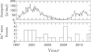
Figure 2. (Top) Monthly sunspot numbers over the course of this study. (bottom) Number of wave events observed during each year of this study.
Download figure:
Standard image High-resolution imageFigure 3 divides every year into tenths and plots the number of events found in that part of the year. November through January do appear to favor observability to a marginal degree, suggesting that the spacecraft is more likely to find a wave event when within the He+ focusing cone. However, the statistics derived from 25 events are poor and this is far from the controlling consideration. It appears that waves are almost equally likely to be found at any part of the year.
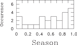
Figure 3. Distribution of events as a function of the time of year.
Download figure:
Standard image High-resolution imageFigure 4 shows the distribution of event durations. A "typical" event lasts from 1 to 3 hr. The nominal correlation time for the solar wind at 1 au is 1 hr in the spacecraft frame, which suggests that event duration is most likely determined by changing solar wind conditions rather than any changes in the source atom density or ionization rate. Since He atoms are ionized primarily by solar EUV, it is possible that large UV flares could produce short-term enhancements in ion production. However, such a transient event would not produce enhancements in ion production or wave excitation that would be localized in space. We have not attempted to establish such a link here.

Figure 4. Distribution of event duration in hours.
Download figure:
Standard image High-resolution imageOf the 25 events in this study, the shortest is just 58 minutes in duration and the longest is almost 7 hr while 1–3 hr is more typical. There may be events of shorter duration, but they appear too similar to the naturally occuring noise in the spectrograms to be reliable. The control intervals used in this study tend to have durations of several hours. They are listed in Table 3. Comparison of the control list to the event list will demonstrate that the control intervals were selected to be in general proximity to the wave events. The control intervals exhibit similar solar wind conditions (flow structure, wind speed, density, temperature, magnetic field strength, etc.) to the wave events as shown below.
Table 3. Control Intervals
| Year/DOY | Year/DOY | Year/DOY | Year/DOY |
|---|---|---|---|
| 1999/179.29–179.50 | 1999/180.46–180.58 | 1999/184.38–184.46 | 1999/185.75–186.00 |
| 1999/188.92–189.00 | 2000/194.50–194.63 | 2000/195.88–196.00 | 2000/196.00–196.13 |
| 2000/261.50–261.58 | 2000/262.75–262.88 | 2000/263.75–263.88 | 2000/332.42–332.54 |
| 2000/332.58–332.67 | 2000/332.88–333.00 | 2000/336.13–336.25 | 2000/366.92–367.00 |
| 2001/108.67–108.83 | 2001/108.88–108.96 | 2001/109.75–109.88 | 2001/223.25–223.42 |
| 2001/224.08–224.21 | 2001/297.08–297.25 | 2001/332.50–332.58 | 2002/139.79–139.92 |
| 2003/270.38–270.46 | 2003/270.58–270.75 | 2004/280.00–280.13 | 2004/317.42–317.50 |
| 2004/318.13–318.25 | 2005/79.75–80.00 | 2005/80.67–80.83 | 2006/100.79–100.92 |
| 2006/101.88–102.00 | 2006/236.92–237.00 | 2008/161.13–161.29 | 2008/161.67–161.83 |
| 2008/344.29–344.54 | 2009/33.21–33.38 | 2009/33.58–33.75 | 2009/236.17–236.33 |
| 2009/236.46–236.71 | 2009/236.88–237.00 | 2009/307.79–308.00 | 2010/14.25–14.50 |
| 2010/14.50–14.75 | 2010/14.75–15.00 | 2010/15.33–15.42 | 2010/15.50–15.75 |
| 2010/15.75–16.00 | 2012/147.38–147.46 | 2012/332.08–332.21 | 2012/332.42–332.50 |
| 2012/333.50–333.63 | 2015/28.50–28.63 | 2015/60.50–60.63 | 2015/60.83–60.96 |
Download table as: ASCIITypeset image
Figure 5 shows the ambient plasma conditions for the 25 wave events and associated control intervals. Top to bottom: the wind speed, VSW, for events is in the normal range of solar wind observations. Although there are times when the control intervals have higher wind speed than the wave events, this is not systematic within the ensemble. The proton densities, NP, are generally lower than the average solar wind density at 1 au (6–8 p+ cm−3), but both wave events and control intervals have similar values. The low densities correspond to the fact that many of the observations exist within rarefaction intervals. Proton temperatures are in the range of average values for 1 au. Again, the temperature of control intervals is comparable to the associated wave events. The magnetic field intensity is typical of 1 au values and generally comparable between wave events and control intervals. The Alfvén speed, VA, is typically high for 1 au values in keeping with the low densities, but not unusual, and both wave events and control intervals are comparable. The angle between the mean magnetic field and the radial direction, ΘBR, is generally <45° for both wave events and control intervals with some exceptions.
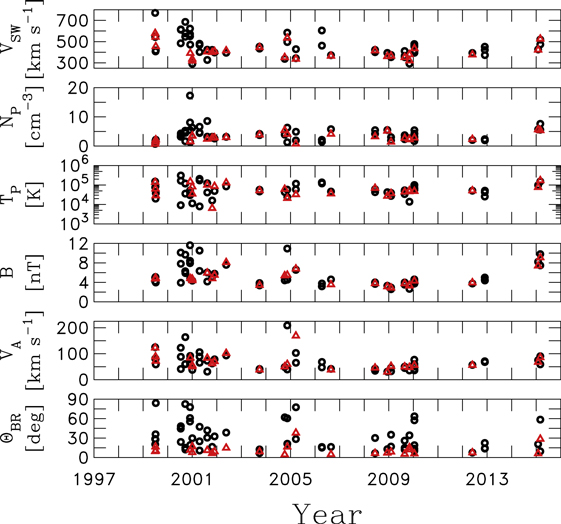
Figure 5. Red triangles represent wave events. Black circles are control intervals. (Top down) Average wind speed, proton density, proton temperature, HMF intensity, Alfvén speed, and angle between the HMF and radial direction.
Download figure:
Standard image High-resolution imageIt is worth taking a closer look at the distribution of ΘBR. Figure 6 shows the distribution for wave events (top) and control intervals (bottom). With the exception of two, all wave events have ΘBR < 20°. Control intervals have a somewhat more extensive distribution to higher values, but their distribution is also peaked at  . The Ulysses observations of waves due to newborn interstellar H+ (Cannon et al. 2014a) showed a distribution of ΘBR that extended to ∼80°, but we do not see that here. Those authors concluded that the larger angles did not prevent the instability from occurring. We suspect that the rarefactions at 1 au which favor wave growth possess more radial fields than those at Ulysses and that this is the reason for the more radial field orientations in the ACE event list rather than a causal relationship between wave growth and field orientation.
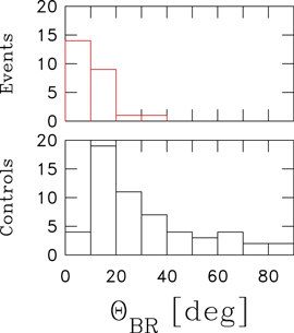
Figure 6. Distribution of angle between minimum variance and mean field directions for both wave events (top) and control intervals (bottom).
Download figure:
Standard image High-resolution image3.3. Wave Analysis
After finding the wave events via the spectrograms, we proceed to analyze the observations using carefully constructed subsets of the data. Figure 7 shows the results of our analysis of the wave event shown in Figure 1. The specific time interval is day 236.79–236.88 in year 2009. Top to bottom, the panels are: the power spectra for the 3 components of the magnetic field rotated into mean field coordinates plus the trace (total power) and the spectrum of  the degree of polarization, Dpol; the coherence, Coh; the ellipticity, Elip; the angle between the minimum variance direction and the mean field, which we again denote as
  and the normalized magnetic helicity, σM (Matthaeus & Smith 1981; Smith 1981; Matthaeus & Goldstein 1982; Matthaeus et al. 1982). The power and magnetic helicity spectra were computed via Blackman–Tukey spectral techniques (Matthaeus & Goldstein 1982; Matthaeus et al. 1982; Leamon et al. 1998b, 1998c; Smith et al. 2006b, 2006c; Hamilton et al. 2008; Markovskii et al. 2008, 2015; Joyce et al. 2010, 2012; Argall et al. 2015; Aggarwal et al. 2016) where a first-order difference of the measurements is used to pre-whiten the data and reduce the effect of leakage (Smith et al. 1990). The resultant spectra are then corrected using a "post-darkening" algorithm (Chen 1989). The polarization spectra were computed via FFT of the time series (Means 1972; Mish et al. 1982). FFT methods were also used to compute the power and helicity spectra, which were found to agree with the spectra shown here. The power and polarization spectra are computed in mean field coordinates (Belcher & Davis 1971; Bieber et al. 1996), while the helicity is, of necessity, computed in standard heliographic coordinates. In the detailed analyses of the wave and control intervals, we compute the minimum variance direction to represent
  instead of the wave normal direction used in the daily spectrograms. For the intervals analyzed here, the results are equivalent.

Figure 7. Spectral analysis of day 236.79–236.88 of 2009. (top down) Power spectra of the components in mean field coordinates including total power and power spectrum of the  timeseries. Note enhanced power at frequencies
  . The spectrum of the field-aligned component, Bz, is obscured by the essentially identical spectrum of
  . The total power within the enhancement exceeds the spectrum of the field-aligned component by ∼10×, consistent with transverse fluctuations. Degree of polarization and coherence are high within the same frequency range. The ellipticity ≃−1 indicating left-hand polarized waves in the spacecraft frame and ΘkB ≃ 0° consistent with parallel propagation. The normalized magnetic helicity ≃+1 and the radial component of the HMF is <0, which is consistent with the measured polarization.
Download figure:
Standard image High-resolution imageBoth  and
and  are marked in the top panel. The power spectra are shown in mean-field coordinates prescribed by (eB × (eR × eB), eR × eB, eB) where eR and eB are the unit vectors in the radial and magnetic field direction, respectively (Belcher & Davis 1971; Bieber et al. 1996). The two components of the magnetic field perpendicular to the mean field are shown in red and green, respectively. The power spectrum of the field-aligned component is shown in blue. The upper black curve is the trace (total power) and the lower black curve is the power in
  . The wave power is strongly enhanced at
  . The bulk of the power in the wave enhancement resides in the perpendicular components meaning that the fluctuations are largely transverse to the mean magnetic field and the angle between the minimum variance direction and mean magnetic field is ∼0°. The two perpendicular components contain nearly identical energy at these frequencies which is indicative of circular polarization. The trace spectrum behaves as f−2 at frequencies
  as predicted (Lee & Ip 1987), but begins to fall more steeply at f > 0.1 Hz.
The degree of polarization and the coherence are both high (near the maximum value 1) in this same frequency range. At greater and lesser frequencies the value of both is small. The ellipticity approaches −1 indicating left-hand circularly polarized fluctuations consistent with waves excited by a beam of newborn interstellar ions moving sunward and parallel to the mean magnetic field. At greater and lesser frequencies Elip ≃ 0. The angle ΘkB ≃ 0 in this frequency range suggests wave propagation parallel to the mean magnetic field. At greater and lesser frequencies ΘkB approaches 90°. Finally, the normalized magnetic helicity approaches +1 and is consistent with the measured ellipticity when the mean field direction is taken into account (Smith et al. 1984). At greater and lesser frequencies  .
.
This analysis is incapable of distinguishing between parallel propagation in the sunward and anti-sunward directions. The ACE/SWEPAM instrument is not fast enough to resolve ion distribution moments at these frequencies and does not provide the necessary solar wind velocity fluctuations needed to discern the propagation direction of these waves.
For each wave event and control interval, we average Dpol, Coh, Elip and ΘkB over the frequency range  . Figure 8 shows the results of that analysis. Both Dpol and Coh show high values ≥+0.75 for wave events and generally smaller values ≃+0.5 for control intervals. Except for two instances, the wave events show Elip < −0.5 and generally ≃−1. This is consistent with left-hand polarized waves in the spacecraft frame. There are two exceptions to this where the waves are right-hand polarized in the spacecraft frame. A similar minority of right-hand polarized waves were reported by Cannon et al. (2014a, 2014b) for waves excited by pickup H+ observed by the Ulysses spacecraft and one such event was reported by Aggarwal et al. (2016) for observations by the Voyager spacecraft in the range 2–6 au. We do not fully understand the reason for these observations, but we believe the source of the observations remain correctly identified as newborn interstellar PUIs. We find no other likely sources for these waves and they do conform to expectations in all other respects. The average Elip for control intervals at these same frequencies is ≃0. The angle between the minimum variance direction,
  , and the mean field direction,
  0, given by ΘkB is generally small for the wave events while values for control intervals are frequently larger. This is consistent with both theory predicting parallel-propagating waves (Lee & Ip 1987) and the presence of transverse fluctuations.
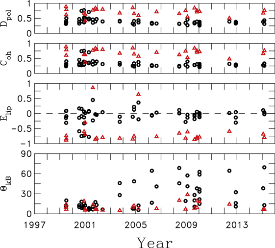
Figure 8. Red triangles represent wave events. Black circles are control intervals. (Top down) Degree of polarization, coherence, ellipticity, and angle between the minimum variance and HMF directions.
Download figure:
Standard image High-resolution imageWe infer the background power spectrum for the wave events by extrapolating from lower frequencies  to frequencies greater than the wave enhancement. In the case of control intervals, we simply use the measured spectrum. Figure 9 (top) shows the resulting background power level as inferred or measured at
  . The background spectrum for the wave events is generally less than the measured spectrum for the control intervals. This means that if wave excitation is the same in either case, the lower background level favors the observability of the waves. However, this relationship is not the last word on the subject of wave observability. Figure 9 (bottom) also shows the ratio of the measured peak wave power to the infered background power at the same frequency. Wave power is typically a factor of 2–10 greater than the background level with a few events exceeding this level of amplification.
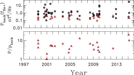
Figure 9. Red triangles represent wave events. Black circles are control intervals. (Top) Background power level measured at  . (Bottom) Ratio of peak wave power to background power for wave events.
Download figure:
Standard image High-resolution image3.4. Excitation and Cascade
We now apply the formalisms developed in Sections 2. The rates and timescales for wave events described here are listed in Table 2. Figure 10 shows the total ionization rates for ISN He (per atom) being the sum of photoionization, electron impact ionization, and charge exchange with solar wind particles. In this analysis we used the Carrington rotation averages of the ionization rates, but we have checked that the use of daily time series does not change the results siginificantly. Note the dependence upon solar cycle with ionization rates being lowest during solar minimum and highest during solar maximum. Both wave events and control intervals follow the same variation with solar cycle and show very little difference between intervals that are closely spaced in time. Comparison of Figures 2 and 10 show an imperfect correlation between the observation rate of wave events and the He ionization rate βHe. Both appear to peak around 2001, but this does not explain the event peak in 2009. At the least, the statistics of small numbers would dictate caution in any effort to over-interpret any perceived correlation between the two plots.

Figure 10. Computed values of the total βHe (photoionization, electron impact ionization, and charge exchange) for wave events (top) and control intervals (bottom). Symbols "+" show the result when only photoionization is considered.
Download figure:
Standard image High-resolution imageFigure 11 shows the computed density of neutral He atoms for the wave events and the control intervals. While the value is generally ∼0.015 cm−3 (Gloeckler et al. 2004), which is the average interstellar value, there are notable times when the computed density is much greater. These occur when the spacecraft is in the gravitational focusing cone. One pair of intervals (one wave and one control interval) show especially high values of ISN He at the end of 2008 when the spacecraft is very near to the center of the cone and the solar cycle is near minimum. Solar minimum brings the weakest intensity of solar EUV which permits the greatest number of neutral atoms to penetrate to 1 au.
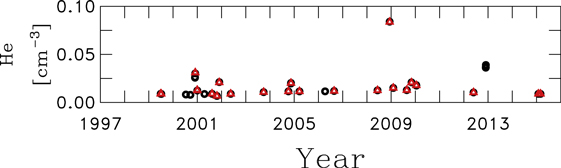
Figure 11. Computed density of ISN He atoms at the times of wave events and control intervals. Wave events are again given by red triangles while control intervals are black circles.
Download figure:
Standard image High-resolution imageThe production rate of ISN He+ ions is the product of the neutral He density and the ionization rate  . This is shown in Figure 12. Most intervals fall at or below ∼2 × 10⁻⁹ cm−3 s−1 while six pairings of wave events and control intervals have significantly greater He+ production rates. These are the same times that show either elevated neutral He densities, elevated He+ ionization rates, or both. In some cases, such as early in 2015, elevated values of βHe are offset by low values of neutral He atom densities and do not show elevated He+ production rates. This is a natural consequence of increased ionization rates reducing the supply of neutral atoms by 1 au. As a result, the solar-cycle dependence seen in Figure 10 is not seen in Figure 12 despite the record low solar EUV and solar wind conditions seen during the recent protracted solar minimum (Smith & Balogh 2008; Didkovsky et al. 2010; McComas et al. 2013; Smith et al. 2013; Didkovsky & Wieman 2014).

Figure 12. Production rate of He+ which is the product of the neutral He density and the ionization rate βHe. Wave events are again given by red triangles while control intervals are black circles.
Download figure:
Standard image High-resolution imageFigure 13 (top) shows the time required for the instability to produce waves of the observed amplitudes using the computed He+ ionization rates given above. All but five wave events achieve their observed wave energy in <40 hr. This does not relate to the event duration, which is a separate matter that describes only the size of the region of space where wave growth is observed. Four intervals require more than 50 hr and one wave event requires what appears to be an unphysically large amount of time to produce the observed wave energy. We can only attribute this exceptionally large value of the wave energy accumulation time to an underestimation of the growth rate due to anomalies in the He+ production rate or variability of the observed plasma conditions prior to observations. Figure 13 (bottom) shows the time required for the instability to produce waves at the observed background level for the control intervals where waves are not seen. Note that in most instances the required accumulation time is <50 hr and is generally comparable to the accumulation time required of the wave events. The instability is not especially weaker during the control intervals. There are exceptions noted on the figure where the computed accumulation time is excessive, but these are the exception rather than the rule. The instability alone does not appear to determine whether waves are seen in the data.

Figure 13. (Top) Accumulation times required for the instability to produce waves at the observed amplitude. (Bottom) Accumulation times required for the instability to produce waves at the observed background level for control intervals.
Download figure:
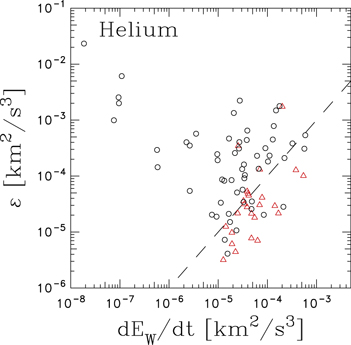
Standard image High-resolution imageFigure 14 compares the growth rate of waves due to the instability caused by the PUI distribution to the turbulent cascade rate for each of the wave events (red triangles) and control intervals (black circles). The former builds up wave energy while the latter destroys the wave and distributes its energy to small scales for dissipation. Although not a perfect organization of the results, most wave events show growth rates that exceed the turbulent cascade rates. Wave growth rates that exceed the turbulent cascade rate constitute the "observability condition" which is required for wave energy to accumulate. Three of the wave events lie demonstrably on the turbulence-dominated side of the figure while four more lie on the line. All seven of these wave events have background spectra >0.3 nT2 Hz−1 at  . While they are not alone in this regard, it does place these events among the highest background levels of all wave events. The remaining 18 wave events lie clearly on the "observable" side of the plot where wave growth exceeds the turbulent cascade. Only 9 of the 56 control intervals show computed growth rates exceeding cascade rates with the remaining 47 control intervals showing turbulent rates that exceed the wave growth rates, as would be expected of an interval without observable wave energy.
Figure 14. Comparison of the wave energy production rate due to the PUI instability vs. the turbulent energy cascade rate as computed from MHD extensions of Kolmogorov theory (Kolmogorov 1941). Wave events are again shown as red triangles while control intervals are black circles.
Download figure:
Standard image High-resolution image
4. SUMMARY
We have shown 25 data intervals when low-frequency waves due to newborn interstellar pickup He+ ions are visible in the ACE/MAG data. Although ACE orbits the L1 Lagrange point, it is unlikely that the reported waves arise from ions accelerated at the Earth's bow shock or within its magnetosphere as He+ is relatively rare in the solar wind, magnetosphere, and Earth's foreshock. Moreover, there is no evidence of in situ acceleration of the source ions given that the wave enhancements are seen exclusively at  . The wave events typically last a few hours with no observations lasting more than 7 hr. There is an enhanced likelihood of observing the waves from November through January, which is a time that brackets ACE's passage through the gravitational focusing cone, but this is not the sole determinant of when the waves are observed. They are also seen throughout the solar cycle though the occurrence rate does appear to correlate with the overall He ionization rate in so far as there are more observations during solar maximum than during solar minimum.
The thermal ion instruments on the ACE spacecraft lack the time resolution that would be needed to determine the expected sunward propagation, but in all but two instances the spacecraft-frame ellipticity is left-handed as is expected for waves due to newborn interstellar pickup ions. High degrees of coherence and polarization are also seen for the waves. The waves are transverse, noncompressive, and with minimum variance directions within 30° of the mean field direction.
The waves are seen when the background spectrum is low and the resultant turbulence is weak. This occurs often, but not exclusively, in rarefaction regions. Densities are often low and flow speeds moderate during the wave events. The mean field is often quasi-radial, pointing to a specific type of rarefaction region discussed by Gosling & Skoug (2002), Murphy et al. (2002), and Schwadron (2002).
We have argued that the overarching determining factor for the observability of the waves is that the wave growth rate due to the instability must exceed the energy cascade rate associated with the turbulence. The waves typically require 5 to 40 hr to accumulate the observed wave energies using theoretical predictions for the instability. This is a significant fraction of the transit time of the wind from the Sun to the Earth. If the instability is not sufficiently strong, the turbulence will absorb the wave energy which will be transported to smaller scales where dissipation will heat the background plasma. This is the normal and expected fate of the wave energy when the waves are not observed. It is argued that the instability is always present, but if it fails to exceed the turbulent cascade rate the waves are not seen and the associated wave energy is used by the turbulence for thermal ion heating. This "observability condition" is rarely achieved so the waves are seldom seen.
It is unlikely that these observations are related to low frequency wave, LFW, storm events (Jian et al. 2010, 2014; Boardsen et al. 2015; Gary et al. 2016). Those events are generally seen at higher frequencies  and have mixed polarization. The spacecraft-frame frequencies are not tied to the source ion gyrofrequencies as far as has been determined. Jian et al. (2014) argue credibly that LFW storm events are not related to newborn insterstellar or cometary pickup ions.
Unsmoothed monthly sunspot numbers were obtained from NOAA at ftp://ftp.ngdc.noaa.gov/STP/. C.W.S. and M.K.F. are supported by Caltech subcontract 44A1085631 to the University of New Hampshire in support of the ACE/MAG instrument. P.A.I. is supported by NASA grant NNX13AF97G and by an NSF SHINE grant AGS1358103. B.J.V. is supported by NSF/SHINE grant AGS1357893. J.M.S. and M.B. acknowledge the support by the Polish National Science Center grant 2015/18/M/ST9/00036. T.H.Z. and J.A.G. are supported, in part, by NASA grant NNX13AH66G. M.K.F. is an undergraduate physics major at UNH. C.J.J. is a graduate student completing his Ph.D. in physics at UNH. M.R.A. is a recent Ph.D. from the UNH program.