ASSESSING MAGNETIC TORQUES AND ENERGY FLUXES IN CLOSE-IN STAR–PLANET SYSTEMS

Close-in giant planets are the most easily detected exoplanets today because they are able to imprint significant radial velocities onto their host star, and generate very clear transits. Due to their proximity, the two main interactions with their host (tides and magnetism, see Cuntz et al. 2000) are very strong compared to the case of solar system planets. In theory, fast and efficient exchanges of angular momentum and energy between the planet and its host are hence possible in these systems, altering their secular evolution. As a result, significant efforts have been made in the past decades to look for observational signatures of these interactions, along with thorough theoretical research to better understand the physical mechanisms sustaining them.

Numerous puzzling observations of close-in systems have been recently reported. Periodic anomalous chromospheric emissions have been observed on stars harbouring a close-in hot Jupiter (Shkolnik et al. 2008). The on/off nature of these emissions suggest either a magnetic origin (Strugarek et al. 2015) or material infall from the orbiting planet (Pillitteri et al. 2015). WASP-18 also possesses a close-in planet, and was reported to present a surprising lack of X-ray emissions (Pillitteri et al. 2014), which could also be accounted for by its interaction with the orbiting planet. Finally, Radio and UV emissions in close-in systems are intensively searched for today (Grießmeier et al. 2007; Fares et al. 2010; Lecavelier des Etangs et al. 2013; Turner et al. 2013). These emissions are difficult to observe because they were not found to induce any statistical observational trend (Poppenhaeger & Schmitt 2011; Miller et al. 2015), likely due to their on/off nature. They may nevertheless be observed for some systems, like HD 189733, for which an excess of absorption was reported during transit (Llama et al. 2013; Cauley et al. 2015). The signal is possibly tracing the existence of a bow shock in front of the orbiting planet created by the magnetohydrodynamical interaction between the planet and the wind of the host star.

The population of exoplanets itself is also affected by star–planet interactions. Stars hosting close-in planets tend to rotate more rapidly than planet-free twin stars (Pont 2009; Maxted et al. 2015). The physical origin of this trend is still debated today, but tides, magnetic interactions, or a combination of both are likely the key to make close-in planets migrate and be absorbed by their host, transferring at the same time significant angular momentum to the star (Zhang & Penev 2014). In addition, a dearth of close-in planets around fast rotators was reported by several authors (McQuillan et al. 2013; Lanza & Shkolnik 2014) using Kepler data. Again, both tides and magnetic interactions could be vectors of angular momentum transfers in such systems, making close-in planets migrate efficiently and explaining this dearth. Finally, some recent observations also report a possbile influence of close-in hot Jupiter on the rotation and magnetic activity of their host (Poppenhaeger & Wolk 2014), albeit larger samples of stars are needed today to confirm these trends.

These observations challenge our understanding of interactions between a close-in planet and its host star. Furthermore, a refined physical description of star–planet interaction is also needed today to guide the hunt for exoplanets. Finally, the anomalous, enhanced emissions (being either in Radios, UV, or X-ray) in such systems likely trace the existence of the magnetic field of the planet. A better theoretical understanding of the physical mechanisms sustaining these emissions could provide a way to characterize the magnetic field of close-in exoplanets with observations, or help us constrain the internal properties of the planet if it does not possess an intrinsic magnetic field, for which we do not have any constrains yet (e.g., Zarka 2007; Strugarek et al. 2015; Vidotto et al. 2015).

Among the means of interactions between a star and close-in planets, tides are by far the most studied aspect. They are known to lead to spin–orbit synchronization (Mathis et al. 2013), planet migration (Bolmont et al. 2012; Baruteau et al. 2014, p. 667; Zhang & Penev 2014; Damiani & Lanza 2015) and star spin-up (Barker & Ogilvie 2011; Ferraz-Mello et al. 2015) due to angular momentum exchange between the planet and the star. Their efficiency was recently shown to depend on the internal structure of both the planet and the hosting star (Auclair-Desrotour et al. 2014; Guenel et al. 2014). While significant insights have been recently gained for tidal gravito-inertial waves (see, e.g., Auclair-Desrotour et al. 2015), the fully nonlinear interactions between tidal waves, and the properties of magneto-gravito-inertial waves, still need to be characterized to obtain a satisfying understanding of angular momentum transfers by tidal waves in planetary and stellar interiors.

The close-in planets also receive intense radiation from their host due to their proximity. The associated ionization of the atmosphere of the planet allows an enhanced atmospheric escape from the planet (Yelle et al. 2008; Owen & Adams 2014; Trammell et al. 2014). Various types of such planetary outflows were found to exist, depending on the properties of the hosting star (Matsakos et al. 2015). If the planet is in a sufficiently close-in orbit, the escaping material may fall on the stellar surface, providing an additional variability to the chromospheric emissions of the star (see, e.g., Pillitteri et al. 2015).

Finally, magnetic fields provide another systematic source of interaction between a star and a close-in planet, often refererred to as "star–planet magnetic interaction" (SPMI). Close-in giant planets are generally thought to orbit inside the Alfvén surface of the wind of their host, i.e., in a region where the local Alfvén speed exceeds the velocity of the wind. This allows for particularly efficient transfers between the planet and its host (Saur et al. 2013; Strugarek et al. 2014) because Alfvén waves carrying energy and momentum are able to travel between the two bodies. Such close-in exoplanet systems are similar to planet–satellite systems in the solar system, with the additional complexity of the existence of a stellar wind. As a result, the superposition of the Alfvénic perturbations triggered by the orbital motion of the planet will form Alfvén wings (Goldreich & Lynden-Bell 1969; Neubauer 1980, 1998) for which the structure depends on the properties of the wind and of the planet magnetic field (if any, see Saur et al. 2013; Strugarek et al. 2015). The SPMIs will generally be a source of planet migration (Laine et al. 2008; Lovelace et al. 2008; Vidotto et al. 2010; Laine & Lin 2011; Strugarek et al. 2014, 2015) and stellar spin-up (Cohen et al. 2010; Lanza 2010; Strugarek et al. 2015). For fast-rotating stars, the magnetic torque can be opposite such as to slow down the hosting star when the planet is beyond the co-rotation radius (see Strugarek et al. 2014). It nevertheless appears to be too weak to fully solve the so-called angular momentum problem for young stars (Bouvier & Cébron 2015). The energy channelled in the Alfvén wings can also be a source of additional heating in the chromosphere of the host (Ip et al. 2004; Preusse et al. 2006; Saur et al. 2013), which could potentially lead to anomalous emissions related to the existence of a close-in planet. This mechanism was recently shown (Strugarek et al. 2015) to naturally provide an on/off source of energy for enhanced emissions.

SPMIs are shaped by the stellar wind of the host star. The plasma conditions in the stellar wind determine whether the SPMI will be super- or sub-Alfvénic. The non-axisymmetry of real stellar magnetic fields can thus cause the SPMI to change as a planet orbits in the wind (Cohen et al. 2015). Observations of the magnetic field (using the Zeeman Doppler Imaging technique, see, e.g., Donati & Landstreet 2009) of planet-hosting stars are thus of great importance to help constrain the possible SPMIs in real systems (e.g., Moutou et al. 2016, for the Kepler-78 system). Dedicated numerical simulations of stellar winds, based on observed magnetic topologies in 3D, are consequently necessary today (Vidotto et al. 2015; Alvarado-Gómez et al. 2016; A. Strugarek et al. 2016, in preparation).

SPMIs also generally depend on the internal structure of the planet (Strugarek et al. 2014). When the planet is not able to sustain its own magnetic field, the stellar wind field is able to permeate into its interior, depending on its internal composition. This interaction, dubbed as unipolar (e.g., Laine et al. 2008; Laine & Lin 2011), can lead to planet inflation due to ohmic dissipation, as well as planet migration due to magnetic torques. In the case of a close-in planet operating a dynamo and sustaining its own magnetosphere, magnetic torques still develop depending on the magnetic topology (Strugarek et al. 2015), and the interaction is then referred to as dipolar.

The aim of this work is to provide a parametrization of the main effects of magnetic interaction in the dipolar case, relevant for (1) the orbital migration of a planet and the associated spin-up (or down) of its host and (2) the existence of enhanced emissions in close-in systems. Our study is built on a 3D magnetohydrodynamical (MHD) global model, in which a magnetized planet is introduced in a close-in orbit in a self-consistently simulated stellar wind. This model will be briefly described in Section 2. We present here a grid of numerical simulations, where we vary the orbital radius of the planet and the strength of its magnetic field. We propose a parametrization of the magnetic torque applied to the planet (Section 3), and of the magnetic energy flux driving enhanced emissions in the system (Section 4). The effect of ohmic dissipation on SPMIs is quantified in Section 5, and we finally summarize and discuss our results in Section 6.

The model used in this work is described in detail in Strugarek et al. (2015). It is based on the MHD formalism to describe the interaction of a magnetized planet with a self-consistently driven stellar wind. The system of equations is written in a frame rotating with the orbiting planet, which enables us to numerically set the orbiting planet at a fixed position in a grid centered on the rotating hosting star. The grid resolution is enhanced around the star (Δx = 0.03 R_⋆) and the planetary magnetosphere (Δx = 0.12 R_P), and the grid is stretched away from the central star elsewhere. The grid used in this work is slightly coarser than in Strugarek et al. (2015), in order to be able to produce a grid of numerical simulations with accessible computational ressources.

The set of MHD equations we solve is

$$\begin{eqnarray}&&{\partial }_{t}\rho +{\boldsymbol{\nabla }}\cdot (\rho {\boldsymbol{v}})=0\end{eqnarray} \tag{ 1 }$$

$$\begin{eqnarray}&&\rho {\partial }_{t}{\boldsymbol{v}}+\rho {\boldsymbol{v}}\cdot {\boldsymbol{\nabla }}{\boldsymbol{v}}+{\boldsymbol{\nabla }}P+{\boldsymbol{B}}\times {\boldsymbol{J}}/(4\pi )=\rho {\boldsymbol{a}},\end{eqnarray} \tag{ 2 }$$

$$\begin{eqnarray}&&{\partial }_{t}P+{\boldsymbol{v}}\cdot {\boldsymbol{\nabla }}P+\rho {c}_{s}^{2}{\boldsymbol{\nabla }}\cdot {\boldsymbol{v}}=4\pi (\gamma -1)({\eta }_{e}+{\eta }_{P}){{\boldsymbol{J}}}^{2},\end{eqnarray} \tag{ 3 }$$

$$\begin{eqnarray}&&{\partial }_{t}{\boldsymbol{B}}-{\boldsymbol{\nabla }}\times ({\boldsymbol{v}}\times {\boldsymbol{B}})=-{\boldsymbol{\nabla }}\times (({\eta }_{e}+{\eta }_{P}){\boldsymbol{J}}),\end{eqnarray} \tag{ 4 }$$

$$\begin{eqnarray}&&{\boldsymbol{\nabla }}\cdot {\boldsymbol{B}}=0,\end{eqnarray} \tag{ 5 }$$

where ρ is the plasma density, v its velocity, P is the gas pressure, B is the magnetic field, a is composed of the gravity, Coriolis, and centrifugal forces, ${c}_{s}=\sqrt{\gamma \,P/\rho }$ is the sound speed (γ is the adiabatic exponent, taken to be equal to the ratio of specific heats and set in this work to 1.05), and ${\boldsymbol{J}}={\boldsymbol{\nabla }}\times {\boldsymbol{B}}$ is the current density. We use an ideal gas equation of state

$$\begin{eqnarray}&&\rho \varepsilon =P/(\gamma -1),\end{eqnarray} \tag{ 6 }$$

where ε is the internal energy per mass. Compared to the model described in Strugarek et al. (2015), we have here added the possibility to introduce ohmic diffusivity. Two types of diffusivities can be used. The first, controlled by the ohmic diffusion coefficient η_P, is a standard ohmic diffusion used only inside the planetary boundary condition mimicking a crude ionospheric layer (for more details, see Strugarek et al. 2015). This standard diffusivity can be viewed as a very simple modeling of the actual Pedersen conductivity, which dominates ohmic dissipation in this region (e.g., Neubauer 1998; Duling et al. 2014). The second, controlled by the ohmic diffusion coefficient η_e, is an enhanced diffusivity, which is restricted to current sheets in the simulations. An activation criterion λ is defined by

$$\begin{eqnarray}&&\lambda =\displaystyle \frac{| {\boldsymbol{J}}| {\rm{\Delta }}x}{| {\boldsymbol{B}}| +\epsilon },\end{eqnarray} \tag{ 7 }$$

where Δx is the maximal size of the local grid cell, and  = 10⁻⁴ ensures that λ does not diverge. The enhanced diffusivity is activated based on the criterion λ as follows (see, e.g., Yokoyama & Shibata 1994; Raeder et al. 1998; Jia et al. 2009; Duling et al. 2014)

$$\begin{eqnarray}{\eta }_{e}=\left\{\begin{array}{ccl}0 & {\rm{if}} & {\lambda }^{2}\lt 1\\ {\lambda }^{2}{\eta }_{a} & {\rm{if}} & 1\leqslant {\lambda }^{2}\leqslant {10}^{3}\\ {10}^{3}{\eta }_{a} & {\rm{if}} & {\lambda }^{2}\gt {10}^{3}\end{array}\right.,\end{eqnarray} \tag{ 8 }$$

where η_a is the anomalous diffusion coefficient. Such enhanced diffusion is very useful to control how the magnetic field reconnects in current sheets, while not affecting the remaining modeled system with an additional spurious ohmic dissipation. In Section 5, we quantify the dependency of the global trends derived with a grid of numerical simulations (see Sections 3 and 4) to the enhanced diffusivity, which can be used to trace the impact of the reconnection efficiency and/or the numerical resolution in other studies.

The MHD equations are discretized and solved using the PLUTO code (Mignone et al. 2007). They are solved using a second-order, linear spatial interpolation coupled to an HLL Riemann solver with a minmod flux limiter. They are advanced in time with a second-order Runge–Rutta method. The solenoidality of B (Equation (5)) is ensured with a constrained transport method (Evans & Hawley 1988), and the magnetic field is decomposed into a background field (composed of two dipolar fields, one for the star and one for the planet).

Pioneering numerical simulations of SPMI were conducted by Ip et al. (2004) in a local domain around a close-in planet for prescribed stellar wind parameters. Inhomogeneities in stellar winds and the detailed global magnetic topology, nevertheless, strongly impact the strength and geometry of SPMIs, which warrants a global modeling of star–planet systems. In particular, the detailed knowledge of the three-dimensional structure of the Alfvén wings developing in the system is needed to calculate the magnetic torque, which applies to a close-in orbiting planet (see Section 3). Cohen et al. (2009) carried out the first 3D global simulations of star–planet systems by including a planet as a boundary layer in a stellar wind numerical model and neglecting the planet orbital motion. This limitation was further alleviated in Cohen et al. (2011) by considering a planetary boundary condition changing position with time to mimic an orbital motion. Here we follow a different route and hold the planet fixed in the numerical grid by solving Equations (1)–(5) in a frame rotating at the orbital rotation rate. Finally, the last particularity of our model lies in its planetary boundary condition: it is designed to mimic the coupling to an ionospheric layer, for which conductive properties affect the strength of the SPMI (see, e.g., Neubauer 1998; Saur et al. 2013; Duling et al. 2014, and Section 5).

In this work, we consider only a dipolar (axisymmetric) magnetic field for the star. The planetary magnetic field is also considered to be a dipole, but can be locally either aligned or anti-aligned with the ambient stellar wind field at the orbital radius. We restrict the present exploration to these two topologies, which are expected to give, respectively, the maximal and minimal magnetic interaction strength (Strugarek et al. 2015). We present here a grid of such numerical simulations, where the orbital radius (four different radii) and the planetary magnetic field (three different amplitudes) are varied for each of the two topologies. We furthermore explored the influence of ohmic diffusion for two of these simulations, giving a total of 36 3D nonlinear simulations in this study. A summary of the parameters of this set of simulations, as well as the main numerical results discussed in the following sections, are given in the Appendix.

By analogy with an obstacle in a flow, the magnetic torque applied to the planet due to SPMI is generally written as (e.g., Lovelace et al. 2008; Vidotto et al. 2009)

$$\begin{eqnarray}&&{ \mathcal T }={c}_{d}\,{R}_{{\rm{o}}}\,{A}_{\mathrm{eff}}\,{P}_{t},\end{eqnarray} \tag{ 9 }$$

where R_o is the orbital radius of the planet, A_eff is the effective obstacle area exposed to the flow, P_t is the total (thermal plus ram plus magnetic) pressure of the wind in the frame, where the planet is at rest, and c_d is a drag coefficient. The right-hand side is conveniently composed of the total angular momentum that can be transferred to an obstacle of cross-section area A_eff, multiplied by c_d. In the case of SPMI, the drag coefficient c_d and the effective area A_eff should generally depend on the topology of the interaction, i.e., on the relative orientations of the orbital motion, the interplanetary magnetic field, and the planetary magnetic field. Due to this complexity, the drag coefficient c_d and the effective interaction area A_eff can be non-trivial to estimate.

Fortunately, most terms in Equation (9) can be directly estimated in our set of numerical simulations. The net torque ${ \mathcal T }$ applied to the planet can be calculated by integrating the angular momentum balance on a sphere encircling the planet (see Appendix A in Strugarek et al. 2015). The total pressure of the wind P_t can naturally be estimated from the plasma conditions in the wind at the planetary orbit in our simulations and can be a priori parametrized from the stellar parameters (Section 3.1). The two remaining parameters, c_d and A_eff, require a careful evaluation in our simulations. We detail their estimation in Sections 3.2 and 3.3 respectively.

3.1. Effective Pressure at the Planetary Orbit

Because we consider planets orbiting inside the Alfvén surface around cool stars, the magnetic pressure of the wind almost always dominates its total pressure (since the wind speed is smaller than the local Alfvén speed). If the dominant topology of the stellar magnetic field is a dipole or a quadrupole, the magnetic pressure also generally dominates the ram pressure ${P}_{\mathrm{ram}}=\rho {v}_{o}^{2}$ (the ram velocity is defined as ${{\boldsymbol{v}}}_{o}={{\boldsymbol{v}}}_{\mathrm{wind}}-{{\boldsymbol{v}}}_{\mathrm{kep}}$ ³ ), even for close-in planets (we recall here that the effective total pressure is evaluated in the frame where the planet is at rest, which is why the keplerian velocity enters the definition of the ram pressure). We show in Figure 1 the magnetic, ram, and thermal components of the total pressure P_t in the wind considered in this work. We indeed observe that the total pressure is dominated by the magnetic component for the close-in planets considered here (R_o < 7 R_⋆). Note, nevertheless, that this is not necessarily true for higher order topologies, and depends strongly on how the density profile falls off in the lower corona.

Zoom In Zoom Out Reset image size

In the case of a dipolar magnetic field, the total pressure P_t at the orbital radius can be approximated by (see the dashed line in Figure 1)

$$\begin{eqnarray}&&{P}_{t}({R}_{o})\sim \displaystyle \frac{{B}_{w}^{2}}{8\pi }\sim \displaystyle \frac{{B}_{\star }^{2}}{8\pi }{\left(\displaystyle \frac{{R}_{\star }}{{R}_{o}}\right)}^{6}.\end{eqnarray} \tag{ 10 }$$

Nevertheless, we will hereafter always consider the total pressure P_t rather than this approximated formulation. When applied to a case where the stellar magnetic field is mainly dipolar and aligned with the rotation axis, one may simply use the approximation in Equation (10).

3.2. Drag Coefficient

The drag coefficient is generally thought to represent—in the case of SPMI—the reconnection efficiency between the stellar wind and the planetary magnetic field, at the boundaries of the planetary magnetosphere or of the Alfvén wings themselves. In some interaction cases, it also depends on the conductivity of the obstacle. In the context of planetary radio emissions in the unipolar interaction case (similar to Io–Jupiter interaction), Zarka (2007) approximated c_d with

$$\begin{eqnarray}&&{c}_{d}^{Z}\sim \displaystyle \frac{{M}_{a}}{\sqrt{1+{M}_{a}^{2}}},\end{eqnarray} \tag{ 11 }$$

where ${M}_{a}={v}_{o}/{v}_{a}=\sqrt{{P}_{\mathrm{ram}}/{P}_{\mathrm{mag}}}$ is the local Alfvénic Mach number near the obstacle (v_a is the local Alfvén speed). They argue that in the case of a dipolar interaction, c_d depends on the conductivity in the ionosphere but takes similar values as in Equation (11). Saur et al. (2013) use a different measure of c_d based on the Pedersen conductance Σ_P (which is the Pedersen conductivity integrated over the ionosphere), which can be approximated by

$$\begin{eqnarray}&&{c}_{d}^{S}\sim {M}_{a}{\left(\displaystyle \frac{{{\rm{\Sigma }}}_{P}}{{{\rm{\Sigma }}}_{P}+2{{\rm{\Sigma }}}_{A}}\right)}^{2}\end{eqnarray} \tag{ 12 }$$

$$\begin{eqnarray}&&\sim {c}_{d}^{Z}{(1+{M}_{a}^{2})}^{1/2}{\left(1+2\displaystyle \frac{{{\rm{\Sigma }}}_{A}}{{{\rm{\Sigma }}}_{P}}\right)}^{-2},\end{eqnarray} \tag{ 13 }$$

where ${{\rm{\Sigma }}}_{A}={c}_{d}^{Z}{c}^{2}/4\pi {v}_{a}$ is the Alfvén conductance (where c is the speed of light).

It is instructive to note that in the limit of small M_a (for which Equation (13) was derived), and for small Σ_A/Σ_P (in this work Σ_A ∼ 10¹² cm s⁻¹, while conservative estimates of Σ_P give a value of the order of 10¹³ cm s⁻¹, see Saur et al. 2013; Duling et al. 2014), both expressions reduce to c_d ∼ M_a. We show M_a and c_d as functions of the orbital radius in Figure 2 for the stellar wind considered here (for more details about the parameters of the simulated stellar wind, see Strugarek et al. 2015). In the remainder of this work, we will denote ${c}_{d}={c}_{d}^{Z}$. We choose here to explicitly separate the impact of ohmic dissipation (through the coefficients η_P and η_e, see Sections 2 and 5) from c_d.

Zoom In Zoom Out Reset image size

3.3. Effective Area of the Interaction

The effective area of interaction in SPMI has been a widely used concept in the past years (see, e.g., Fleck 2008; Lovelace et al. 2008; Vidotto et al. 2014; Bouvier & Cébron 2015, and references therein). It is generally viewed as an effective obstacle area A_eff, and is often approximated by a magnetospheric size obtained from a simple pressure balance between the planetary magnetosphere and the wind pressure, which gives

$$\begin{eqnarray}&&{A}_{\mathrm{obst}}=\pi {R}_{\mathrm{obst}}^{2}=\pi {R}_{P}^{2}{{\rm{\Lambda }}}_{P}^{1/3},\end{eqnarray} \tag{ 14 }$$

where we define ${{\rm{\Lambda }}}_{P}={B}_{P}^{2}/8\pi {P}_{t}$ as this pressure ratio. However, as argued in Strugarek et al. (2015), the effective area depends strongly on the topology of the interaction, and is not well approximated by A_obst in the aligned case. The effective area of the interaction can be deduced from Equation (9) in our set of numerical simulations by writing

$$\begin{eqnarray}&&{A}_{\mathrm{eff}}=\displaystyle \frac{{ \mathcal T }}{{P}_{t}{R}_{o}{c}_{d}},\end{eqnarray} \tag{ 15 }$$

where ${ \mathcal T }$ and P_t are directly computed from the numerical simulation and c_d is computed using Equation (11). We fit the deduced effective area as a function of Λ_P and M_a through

$$\begin{eqnarray}&&{A}_{\mathrm{eff}}={A}_{0}\,{{\rm{\Lambda }}}_{P}^{\alpha }\,{M}_{a}^{\beta }.\end{eqnarray} \tag{ 16 }$$

The deduced areas in our set of simulations are shown in Figure 3 for anti-aligned (circles) and aligned (diamonds) cases, as a function of the pressure ratio Λ_P (upper panel) and Alfvénic Mach number M_a (lower panel). The fits (Equation (16)) are shown by the red (aligned) and blue (anti-aligned) dotted lines, and the numerical values are given in Table 1.

Zoom In Zoom Out Reset image size

Table 1.  Fitted Coefficients of the Effective Area of Interaction

Interaction	A0 $[\pi {R}_{P}^{2}]$	α	β
Anti-aligned	3.5 ± 0.3	0.28 ± 0.01	0.02 ± 0.04
Aligned	10.8 ± 0.4	0.28 ± 0.01	−0.56 ± 0.02

Note. The effective area A_eff is fitted using Equation (16).

Download table as:  ASCIITypeset image

The effective area of interaction increases with Λ_P with an exponent α ∼ 0.28 in all cases, which is close to the one-third exponent expected from a simple pressure balance (Equation (14), shown by the dotted black line). In both types of interactions, the effective area is larger than the predicted obstacle area A_obst. In the aligned case, this is awaited (Strugarek et al. 2015) as the effective area incorporates a part of the Aflvén wings themselves (we will come back to this point below). In the anti-aligned case, though, the effective area is systematically higher than the naïve estimation from pressure balance. This is due to the fact that the interaction between the magnetosphere and the stellar wind leads to a compression of the magnetosphere at the nose of the interaction, and a subsequent widening of the magnetosphere perpendicular to the flow v_o, which results in the tear-like shape for the magnetosphere on the equatorial plane. This phenomenon is illustrated on the left panels of Figure 4 for an anti-aligned case, where the magnetic field lines in the plane perpendicular to ecliptic plane are shown in the upper panel, and the streamlines of the flow (in the frame where the planet is at rest) in the ecliptic are shown in the bottom panel. The obstacle size deduced from Equation (14) is shown by the thick black circles. The magnetosphere exceeds the naive obstacle size, and on the ecliptic the compressed tear-like shape of the magnetosphere appears clearly.

Zoom In Zoom Out Reset image size

The effective area of the interaction also strongly depends on the Alfvénic Mach number M_a in the aligned case (β ∼ −0.5, see Figure 3), while it has merely no incidence on A_eff in the anti-aligned cases (the exponent 0.02 in this case is not significant, see Table 1). The origin of this dependency lies in the type of obstacle that develops in the aligned case. In this case, the "open" magnetic field lines at the pole of the planet (which we suppose to be anchored to the planet), face the stellar wind and henceforth have to be considered as part of the planetary obstacle. As a result, the effective area depends on the inclination angle of the Alfvén wings, which is controlled by M_a, and the effective area in the aligned case must also depend on M_a, as observed in Figure 3.

Though, should the full Alfvén wing cross-section be considered as the effective obstacle area (e.g., Fleck 2008)? In fact, the situation is slightly more complicated and can be understood as follows (see schematics in the upper panels of Figure 5). The Alfvén wings are populated by Alfvénic perturbations triggered on the ecliptic plane at the magnetopause, where the stellar wind magnetic field and the planetary magnetic field reconnect (see the current sheet in the lower right panel of Figure 4). If one follows the trajectory of such a perturbation launched at the nose of the reconnecting region (panel (a) in Figure 5), by the time the wind plasma has swept around the planetary magnetosphere on the ecliptic plane (panel (b)) the perturbation has travelled a given distance along the Alfvén wing (panel (c)). This distance defines the portion of the Alfvén wings that is relevant for the angular momentum extraction from the planetary orbit by the magnetic interaction. We show in panel (d) the flow in the ecliptic plane and the Alfvén characteristics out of it with a 3D view for an aligned case. The reconnection area on the ecliptic plane is traced by the orange region showing Λ, as in Figure 4. In order to support this interpretation, we a posteriori calculate the cross-section of the Alfvén wings that corresponds to the measured effective area of the interaction A_eff in this case. This area is shown by the blue and red areas in panel (e) (we have two areas here since interaction develops two Alfvén wings). Using these Alfvén wing areas we can associate a travel distance [d(A_eff)] from the reconnection site on the ecliptic plane, which corresponds to a travel time τ_t of the Alfvénic perturbations up to such a distance along the Alfvén wings, given by

$$\begin{eqnarray}&&{\tau }_{t}={\int }_{0}^{d({A}_{\mathrm{eff}})}\displaystyle \frac{{ds}}{{c}_{A}^{-}}\end{eqnarray} \tag{ 17 }$$

for the northern Alfvén wing, where ds is the infinitesimal distance along the Alfvén wing, and ${{\boldsymbol{c}}}_{A}^{-}={{\boldsymbol{v}}}_{0}-{{\boldsymbol{v}}}_{a}$ is the corresponding Alfvén characteristic. Considering that the plasma sweeps around the magnetospheric obstacle with an average velocity v₀ on the ecliptic plane, we can deduce what should be the extent of the magnetospheric obstacle in the stream direction [${d}_{\parallel }$] to account for an effective area of interaction A_eff by

$$\begin{eqnarray}&&{d}_{\parallel }=\displaystyle \frac{{v}_{o}}{{\tau }_{t}}.\end{eqnarray} \tag{ 18 }$$

We report this deduced distance on the lower right panel in Figure 4. We recall here that we deduced ${d}_{\parallel }$ only from the effective area of interaction A_eff (Equation (15)), and from the shape of the Alfvén wings (to estimate τ_t). We observe that ${d}_{\parallel }$ is indeed an excellent approximation of the size of the magnetospheric obstacle in the stream direction (see Figure 4), validating our interpretation of the effective area of interaction in the aligned case of the close-in star–planet interaction (Figure 5). We recall that in the anti-aligned case, the magnetosphere is closed and this interpretation naturally does not apply.

Zoom In Zoom Out Reset image size

Our sample of simulations also include super-Alfvénic cases, shown in magenta in Figure 3. In the aligned case, they seem to follow the same trend as the sub-Alfvénic cases. The effective area appears to drop for the anti-aligned cases, certainly due to the appearance of a shock in front of the magnetospheric obstacle. This warrants further investigation of the sub- to super-Alfvénic transition of the interaction. We intend to explore this transition in a future work.

The magnetic torque that develops in close-in star–planet systems can hence be parametrized using a combination of Equations (9) and (16), with different exponents (listed in Table 1) depending on the magnetic topology of the interaction topology. The migration timescale of the planet due to the magnetic interaction can subsequently be calculated as follows.

$$\begin{eqnarray}&&{\tau }_{\mathrm{mig}}=\displaystyle \frac{2{J}_{P}}{{ \mathcal T }},\end{eqnarray} \tag{ 19 }$$

where ${J}_{P}={M}_{P}{({{GM}}_{\star }{R}_{{\rm{o}}})}^{1/2}$ is the orbital angular momentum of the planet and the factor of two accounts for the ${R}_{{\rm{o}}}^{1/2}$ dependancy of J_P. Note that the magnetospheric obstacle on the ecliptic plane may also depend on the reconnection efficiency of magnetic field lines in the current sheet that develops. We will detail this aspect in Section 5.2, and conclude on the generic parametrization of the magnetic torque ${ \mathcal T }$ in Section 6.

The Alfvén wings also channel energy between the planet and the star in the form of Alfvén waves. The energy flux can be quantified by the Poynting flux in the Alfvén wing, given by

$$\begin{eqnarray}&&{S}_{a}=\displaystyle \frac{c{\boldsymbol{E}}\times {\boldsymbol{B}}}{4\pi }\cdot \displaystyle \frac{{{\boldsymbol{c}}}_{A}^{\pm }}{| {{\boldsymbol{c}}}_{A}^{\pm }| },\end{eqnarray} \tag{ 20 }$$

where $c{\boldsymbol{E}}=-{\boldsymbol{v}}\times {\boldsymbol{B}}$ is the electric field in the ideal MHD approximation and ${{\boldsymbol{c}}}_{A}^{\pm }$ are the Alfvén characteristics. The power ${ \mathcal P }$ associated with the Poynting flux can be simply obtained by integrating S_a over the Alfvén wing cross-section (for more details, see Strugarek et al. 2015),

$$\begin{eqnarray}&&{ \mathcal P }={\left\langle \int {S}_{A}d{{\rm{\Sigma }}}_{\mathrm{wing}}\right\rangle }_{A}.\end{eqnarray} \tag{ 21 }$$

In order to estimate the accessible power for radio emissions in star–planet systems, Zarka (2007) proposed the following formulation

$$\begin{eqnarray}&&{ \mathcal P }\sim {c}_{d}{S}_{w}{A}_{\mathrm{obst}},\end{eqnarray} \tag{ 22 }$$

where ${S}_{w}={v}_{0}{B}_{w}^{2}/4\pi$ is the incident Poynting flux of the stellar wind. In a more recent study, and in the context of aligned configurations, Saur et al. (2013) found analytically a slightly different formulation, which can be written as

$$\begin{eqnarray}&&{ \mathcal P }\sim {c}_{d}^{S}{S}_{w}{A}_{\mathrm{obst}},\end{eqnarray} \tag{ 23 }$$

where c_d^S is defined in Equation (12).

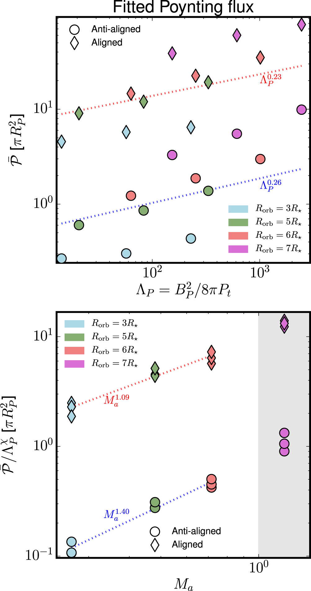
In our simulations, we know a priori the values of c_d (see Section 3.2) and S_w. We hence follow the same procedure as in Section 3 (see Equation (16)) and fit the following normalized total Poynting flux with

$$\begin{eqnarray}&&\bar{{ \mathcal P }}=\displaystyle \frac{{ \mathcal P }}{{c}_{d}{S}_{w}}={A}_{1}{{\rm{\Lambda }}}_{P}^{\chi }{M}_{a}^{\xi }.\end{eqnarray} \tag{ 24 }$$

The fitted coefficients are shown in Table 2 and the resulting fits in Figure 6. The expression of the Poynting flux proposed in the literature (Equations (22) and (23)) directly depend on the obstacle area, in a similar fashion as the torque derived in Section 3. As a result, it can be surprising that in our simulations the Poynting flux appears to vary with Λ_P with a slightly weaker exponent than the torque. Note nonetheless that within the error bars of the two fits, one may consider a common exponent for the two expressions, i.e., α ∼ χ ∼ 0.27. It is remarkable that all simulations, including the two different topologies, can be approximated with a single exponent for the dependancy upon Λ_P. This shows the robustness of the primary source of the magnetic star–planet interaction under various situations, which is characterized by the pressure balance between the ram pressure of the impacting wind and the magnetic pressure of the magnetospheric obstacle.

Zoom In Zoom Out Reset image size

Table 2.  Fitted Coefficients of the Normalized Total Poynting Flux in one Alfvén wing

Interaction	A1 $[\pi {R}_{P}^{2}]$	χ	ξ
Anti-aligned	0.8 ± 0.2	0.26 ± 0.03	1.40 ± 0.10
Aligned	9.7 ± 2.8	0.23 ± 0.04	1.09 ± 0.13

Note The total Poynting flux $\bar{{ \mathcal P }}$ is fitted using Equation (24).

Download table as:  ASCIITypeset image

In contrast with the magnetic torque, the Poynting flux depends on M_a in both the aligned and anti-aligned cases (lower panel in Figure 6). Previous estimates of the Poynting flux (Equations (22) and (23)) imply that $\bar{{ \mathcal P }}$ only depends on the effective obstacle area. In Zarka (2007), the obstacle is the simplified magnetospheric obstacle A_obst (Equation (14)), and as result their scaling law $\bar{{ \mathcal P }}$ only depends on Λ_P. We already saw that—at least in the aligned case–the obstacle estimation (Equation (14)) is not satisfying, hence we do not expect our results to follow Equation (22). In Saur et al. (2013), the effective area appearing in Equation (23) corresponds to the cross-section of the Alfvén wing itself. This cross-section is not trivial to estimate without calculating the nonlinear interaction between the planet magnetosphere and the stellar wind. Our numerical results provide a simple parametrization of the dependancy of this area to the wind Alfvénic Mach number M_a, as shown in the lower panel of Figure 6. They allow us to extend the scaling law derived by Saur et al. (2013) by clarifying an additional dependancy of the cross-section area of the Alfvén wings.

The fact that $\bar{{ \mathcal P }}$ depends on M_a in the anti-aligned case can appear counter-intuitive. In fact, one has to remember that we quantify here the energy flux channelled through the wings. Since the wings themselves depend on M_a, $\bar{{ \mathcal P }}$ is expected to depend on M_a in all cases. This was not the case for the magnetic torque in the anti-aligned cases, as in these cases the torque applies mainly on the magnetospheric obstacle rather than the Alfvén wings themselves.

Up to this point, we have not yet considered the important aspect of ohmic dissipation in our discussion. Because all of the simulations carried out in this work have equivalent numerical resolutions around the planetary magnetosphere, we expect the scaling laws we derived in Sections 3 and 4 to hold up to different dissipation properties. Nonetheless, we expect the multiplicative coefficients of the scaling laws (A₀ and A₁) to be sensitive to dissipation. We now quantify this effect.

We have considered so far only cases with no explicit dissipation (η_P = η_e = 0 in Equations (3) and (4)), letting the numerical scheme set the level of dissipation in our simulations. We explore here two important aspects of ohmic dissipation that can affect the scaling laws derived in Sections 3 and 4. We first explore the influence of ohmic dissipation [η_P] in the ionospheric boundary layer of our model (Section 5.1). We then turn to the effect of anomalous ohmic dissipation [η_e] that is triggered automatically (see Equation (8)) in strong currents sheets in our model (Section 5.2).

5.1. Dissipation in the Ionosphere

We first consider an enhanced ohmic dissipation coefficient η_P in our planetary boundary condition, mimicking a crude ionospheric layer. The ohmic diffusion coefficient can be related to the integrated Pedersen conductivity by (see, e.g., Duling et al. 2014)

$$\begin{eqnarray}&&{\eta }_{P}\simeq {{Hc}}^{2}\,{(4\pi {{\rm{\Sigma }}}_{P})}^{-1},\end{eqnarray} \tag{ 25 }$$

where H stands for the characteristic height of the atmosphere (or ionosphere) of the exoplanet. Both the Pedersen conductivity Σ_P and H are observationally unconstrained for close-in planets possessing an ionosphere. Conservative estimates of both parameters (based on solar system planets and moons) lead to ohmic diffusion coefficients between 10¹³ and 10¹⁶ cm² s⁻¹ (see Kivelson et al. 2004; Saur et al. 2013; Duling et al. 2014). In order to alleviate the degeneracy of our scalings laws with respect to η_P, we report here on a series of simulations with R_o = 6 R_⋆ and Λ_P ∼ 60 for which we systematically increased η_P up to 10¹⁷ cm² s⁻¹. The resulting effective area of the interaction A_eff (Equation (15)) and normalized Poynting flux $\bar{{ \mathcal P }}$ (Equation (24)) are shown in Figure 7 for the aligned (diamonds) and anti-aligned (circle) cases.

Zoom In Zoom Out Reset image size

We first notice that the anti-aligned cases are largely insensitive to η_P. Indeed, in the anti-aligned cases, the planetary magnetosphere is closed and only a few field lines are able to reconnect between the polar cap of the planet and the ambient wind. As a result, the resistivity in the ionospheric boundary layer is largely unimportant in those cases. The aligned cases show a weak dependency upon η_P, shown by the black dashed line in each panel. This trend allows us to estimate that η_P ≃ 8 × 10¹⁴ cm² s⁻¹ in our reference models with no explicit diffusivities.

As η_P is decreased (which here could be achieved by reducing the grid size, for an increased computational cost), the associated Pedersen conductance increases and finally ends up dominating over the Alfvén conductance Σ_A (see Equation (13)). In this case, the interaction is supposed to saturate, with an effective drag that can be approximated by M_a. Given that both the torque and the Poynting flux depend weakly on η_P, our set of simulations already give robust estimates of both effects.

Nevertheless, depending on the star–planet system one is interested in, the ohmic dissipation coefficient η_P (when estimated from adequate modeling of the exoplanet ionosphere) can be added to our scaling laws of the magnetic torque and Poynting fluxes. We now turn to the stronger effect of an anomalous resistivity in the strong current sheets developing due to the magnetic interaction.

5.2. Dissipation in Reconnecting Current Sheets

We now turn to a series of simulations where we activate the enhanced dissipation η_e (Equation (8)) controlled by the ohmic diffusion coefficient η_a. This enhanced dissipation activates only in strong current sheets that develop in the simulation. It is designed to mimic a fast reconnection process that would otherwise be completely controlled by the unavoidable (and slow) numerical dissipation of the numerical scheme.

We show the effective area of interaction and the normalized Poynting flux in Figure 8. The layout is the same as in Figure 7, with the horizontal axis representing the anomalous ohmic diffusion coefficient η_a. We first note that for either the aligned or anti-aligned cases, the effective area of interaction is only mildly affected by the enhanced dissipation. The reconnection rate between the planetary and wind magnetic fields has indeed little impact on the shape of the obstacle, and hence does not affect much of the torque that applies to the planetary obstacle. In the aligned case, the anomalous dissipation nevertheless changes slightly the size of the magnetospheric obstacle in the stream direction (see bottom right panel in Figure 4). A larger dissipation tends to extend spatially the currents sheets (while reducing their strength), leading to an effective increase of the stream-wise size ${d}_{\parallel }$ of the obstacle, and consequently of A_eff. Our simulations suggest that the effective area changes roughly proportionally to ${\eta }_{a}^{0.04}$ in the aligned case (more simulations would be needed to determine this exponent more accurately).

Zoom In Zoom Out Reset image size

While anomalous diffusion has only a small effect on the magnetic torque that applies to the planet, the Poynting flux generated by the magnetic interaction is strongly affected by it (lower panel in Figure 8). In the anti-aligned case, the closed magnetosphere makes the reconnection sites located primarily near the poles of the planetary magnetic field, restricted to a small area. In this case, the Poynting flux is carried by perturbations launched from those sites, and as a result turns out to be very sensitive to magnetic field reconnection there. The Poynting flux in the aligned cases presents a significantly weaker (though not negligible) dependancy to η_a ($\propto {\eta }_{a}^{-0.27}$). This weaker dependancy reflects the change in topology: in the aligned case, the interface between the magnetosphere and the stellar wind on the ecliptic plane is the main reconnection site of the interaction. Its shape, size, and properties are hence primarily set by the pressure balance shaping the magnetospheric obstacle (see Section 3.3), and the reconnection efficiency controlled by η_a then adds second-order effects to its shape and size. As a result, the Poynting flux in the aligned case is less sensitive than in the anti-aligned case, for which the reconnection site is almost completely controlled by η_a. Finally, it is interesting to note that the Poynting flux systematically decreases with the anomalous diffusion coefficient. This relatively strong dependency warrants further investigation of the close-in SPMIs using more realistic magnetic reconnection models. We intend to return to this aspect in a future publication, in particular, for the aligned topologies for which SPMIs could provide an innovative mean of characterizing the magnetic fields of exoplanets.

In this work, we have explored a parametrization of the effects of SPMI in close-in systems in the dipolar case. We have parametrized the magnetic torque applied to the planet, and the magnetic energy flux that can be channeled toward the star due to this interaction. Thanks to a grid of numerical simulations spanning various planetary orbits, planetary magnetic fields, and dissipation properties, we propose the following generic parameterizations

$$\begin{eqnarray}&&{ \mathcal T }={A}_{0}\pi ({c}_{d}{P}_{t}{M}_{a}^{\beta }{\bar{\eta }}_{a}^{{\nu }_{1}})\cdot ({R}_{P}^{2}{R}_{o}{\bar{\eta }}_{P}^{{\nu }_{2}})\cdot ({{\rm{\Lambda }}}_{P}^{\alpha }),\end{eqnarray} \tag{ 26 }$$

$$\begin{eqnarray}&&{ \mathcal P }={A}_{1}\pi ({c}_{d}{S}_{w}{M}_{a}^{\xi }{\bar{\eta }}_{a}^{{\nu }_{3}})\cdot ({R}_{P}^{2}{\bar{\eta }}_{P}^{{\nu }_{4}})\cdot ({{\rm{\Lambda }}}_{P}^{\chi }).\end{eqnarray} \tag{ 27 }$$

The two formulations are separated into groups of parameters depending only on the wind properties (first parenthesis), the planet properties (second parenthesis), and a combination of both (third parenthesis). The exponents appearing in these formulations are given in Tables 1 and 2, and in Figures 7 and 8 for ${\nu }_{1-4}$. They depend on the topology of the interaction, and are given here for the two extreme cases of aligned (strong interaction) and anti-aligned (weak interaction) topologies. As a result, these generic formulations can be used in combination with observational data.

Formulations (26)–(27) can furthermore be used in combination with independent stellar wind models. As an example, one could use a simple potential field extrapolation technique (Schrijver & DeRosa 2003; Réville et al. 2015) to derive the magnetic properties of the stellar wind of a given star, and further use the torque and Poynting fluxes formulations proposed in this work to estimate the migration timescale and accessible energy fluxes for particular close-in star–planet systems.

We have furthermore explored the dependency of our results upon ohmic dissipation in the planet ionosphere (Section 5.1) and in the reconnecting sites (Section 5.2). We have introduced the normalized ohmic dissipation coefficients ${\bar{\eta }}_{a}$ and ${\bar{\eta }}_{P}$, which are the physical dissipation coefficients normalized to the numerical dissipation coefficients deduced from our set of simulations. A normalizing ohmic dissipation coefficient η₀ ≃ 10¹⁵ cm² s⁻¹ can be used as a first approximation in all cases (see Section 5 for details). In combination with the numerical values of the multiplicative factors A₀ and A₁, that were derived for a given numerical resolution, these normalized ohmic dissipation coefficients make the formulations independent of our grid resolution.

We have shown that in the aligned case of the dipolar interaction, the effective area of the interaction is not well approximated by the classical magnetospheric obstacle. We demonstrated that it could be viewed as a portion of the Alfvén wings developing due to the magnetic interaction. The exact subpart of the wings that composes the effective area depends on the elongation of the magnetosphere of the planet in the stream direction, as schematized in Figure 5. As a result, the magnetic torque applied to the orbiting body can be much larger than if it was only applied to a simple magnetospheric obstacle.

Our estimates of the magnetic torque (Equation (26)) can readily be implemented in secular evolution models involving close-in planets, to be systematically compared to tidal migration (e.g., Bolmont et al. 2012; Zhang & Penev 2014). Various topologies and magnetic field amplitudes can easily be considered. Coupled to simple stellar wind models, our formulation allows us to determine possible synthetic populations of exoplanets accounting for the magnetic interactions, which could be compared to the actual distribution of close-in exoplanets observed today.

The Poynting flux formulation (Equation (27)) can be used to estimate potentially observable traces of SPMIs in distant systems (e.g., Saar et al. 2004). Thanks to the versatile formulation presented here, the cases of aligned and anti-aligned configurations can be easily considered, a quantitative estimate of the energy flux originating from the magnetic interaction can be obtained, and the dependancy upon the ionospheric properties of the planet can be incorporated. In combination with dedicated stellar wind models for real non-axisymmetric magnetic configurations, the Poynting flux (Equation (27)) can be applied to estimate the energy source that could drive enhanced emissions on particular stars hosting close-in planets. In turn, the observations of such enhanced emissions could be combined with our estimate of the Poynting flux to infer the possible magnetic field of observed exoplanets (for a first step in this direction, see A. Strugarek et al. 2016, in preparation).

Finally, some caveats need to be mentioned before using the scaling laws derived in this work. First, our modeling of the ionosphere of the planet remains very crude at this stage. A more detailed ionospheric coupling (see, e.g., Goodman 1995; Merkin & Lyon 2010) could be implemented to incorporate more realistic current distributions in the ionosphere, and inhomogeneous Pedersen conductance profiles that likely arise in the tidally synchronized close-in system due to the day/night asymmetry. Second, the sensitivity of the simulated Poynting flux to an anomalous ohmic diffusion warrants further investigations with more realistic magnetic reconnection models. We aim to study the implications of these aspects for the scaling laws derived here in a future work. Finally, we have focused here on the cases of planets sustaining their own magnetic field. SPMIs can also develop in cases where the planet does not possess an intrinsic magnetic field, nor an ionosphere (see, e.g., Laine et al. 2008; Laine & Lin 2011; Strugarek et al. 2014). When applying the scaling laws to real systems, the possibility that the exoplanet does not operate a dynamo shall always be considered along the dipolar interaction scenario. We also wish to explore this unipolar regime with numerical simulations in a future publication.

I want to thank J. Bouvier, A. S Brun, D. Cébron, S. P. Matt, V. Réville, and P. Zarka for stimulating discussions about star–planet interactions. I also want to thank A. Mignone and his team for giving the PLUTO code to the research community. I acknowledge support from the Canadian Institute of Theoretical Astrophysics (National Fellow), and from the Canadas Natural Sciences and Engineering Research Council. This work was also supported by the ANR 2011 Blanc Toupies and the ERC project STARS2. I acknowledge access to supercomputers through GENCI (project 1623), Prace, and ComputeCanada infrastructures.

In this appendix, we give the critical parameters of all the models and the numerical results of the effective area A_eff and normalized Poynting flux $\bar{{ \mathcal P }}$ in Table 3. We remind the reader that the simulated stellar wind is driven by a normalized sound speed ${c}_{s}/{v}_{\mathrm{esc}}=0.222$ corresponding to a coronal temperature of 10⁶ K for a solar-like star. The rotation rate of the central star is defined by the velocity ratio v_rot/v_esc = 3.03 10⁻³, and the dipolar magnetic field of the star by a normalized Alfvén speed of v_A/v_esc = 1 (for more details, see Strugarek et al. 2015).

Table 3.  Numerical Simulations Parameters and Results

Case	Ro [R⋆]	Ma	ΛP	ηP [cm2 s−1]	ηa [cm2 s−1]	Aeff [$\pi {R}_{P}^{2}$]	$\bar{{ \mathcal P }}$ [$\pi {R}_{P}^{2}$]
						Anti-aligned, Aligned	Anti-aligned, Aligned
1	⋯	⋯	14.30	⋯	⋯	7.64, 47.99	0.27, 4.56
2	3.00	0.27	57.19	0.	0.	10.09, 71.45	0.30, 5.74
3	⋯	⋯	228.77	⋯	⋯	15.23, 105.88	0.43, 6.45
4	⋯	⋯	20.77	⋯	⋯	8.15, 30.35	0.60, 9.05
5	5.00	0.48	83.08	0.	0.	11.67, 56.54	0.86, 12.00
6	⋯	⋯	332.30	⋯	⋯	18.07, 87.82	1.38, 19.22
7	⋯	⋯	63.34	⋯	⋯	10.62, 42.24	1.23, 14.61
8	6.00	0.72	253.34	0.	0.	16.17, 62.26	1.87, 22.51
9	⋯	⋯	1013.37	⋯	⋯	24.77, 92.80	2.99, 35.01
10	⋯	⋯		1.6 1015	⋯	10.65, 41.51	1.38, 13.93
11	6.00	0.72	63.34	1.6 1016	0.	10.61, 38.98	1.37, 12.58
12	⋯	⋯		1.6 1017	⋯	310.58, 6.04	1.36, 9.76
13	⋯	⋯		⋯	1.6 1015	10.18, 42.26	1.14, 13.94
14	6.00	0.72	63.34	0.	8.8 1015	10.91, 45.76	0.16, 9.45
15	⋯	⋯		⋯	1.6 1016	10.62, 46.21	0.04, 7.28
16	⋯	⋯	153.26	⋯	⋯	10.15, 43.52	3.30, 38.72
17	7.00	1.20	613.03	0.	0.	15.46, 65.58	5.52, 60.06
18	⋯	⋯	2452.14	⋯	⋯	23.50, 97.20	9.89, 77.87

Note. The input of the simulations is listed on the left side of the table and the results (i.e., the effective area of the interaction and the normalized Poynting flux) on the right. Each case can be either anti-aligned or aligned depending on the orientation of the planetary magnetic field. Results (two last columns) are given for the two topologies in each of the 18 cases, separated by a comma. The local Alfvénic Mach number at the orbital radius is M_a = v_o/v_a, where v_o is the relative motion between the planet and the ambient wind and v_a is the local Alfvén velocity. The pressure ratio between the planetary magnetosphere and the stellar wind total pressure at the orbital radius is ${{\rm{\Lambda }}}_{P}={B}_{P}^{2}/8\pi {P}_{t}$. The effective area A_eff of the interaction and the normalized Poynting flux $\bar{{ \mathcal P }}$ are, respectively, defined in Equations (15) and (24).

Download table as:  ASCIITypeset image