


ABSTRACT
Sunspot cycles usually present a double-peak structure. This work is devoted to using a function to describe the shape of sunspot cycles, including bimodal cycles, and we find that the shape of sunspot cycles can be described by a binary mixture of Gaussian functions with six parameters, two amplitudes, two gradients of curve, and two rising times, and the parameters could be reduced to three. The fitting result of this binary mixture of Gaussian functions is compared with some other functions used previously in the literature, and this function works pretty well, especially at cycle peaks. It is worth mentioning that the function can describe well the shape of those sunspot cycles that show double peaks, and it is superior to the binary mixture of the Laplace functions that was once utilized. The Solar Influences Data Analysis Center, on behalf of the World Data Center, recently issued a new version (version 2) of sunspot number. The characteristics of sunspot cycles are investigated, based on the function description of the new version.
Export citation and abstract BibTeX RIS
1. INTRODUCTION
The function description of the sunspot number variation in a solar cycle of 11 yr (Li 2009; Hathaway 2015) has a far-reaching significance for space weather analysis, operations of low-Earth-orbiting satellites, and so on, especially in the information era. Hathaway et al. (1994) suggested the following four-parameter quasi-Planck function (named function-P in the following), similar to that of Stewart & Panofsky (1938), but with a cubic power law of time and a Gaussian for the decline time:

where parameter a represents the amplitude of a cycle, t0 denotes the starting time, b is related to the rise time, and c is the asymmetry of the cycle. This function could be reduced to a two-parameter (the amplitude and the starting time of a cycle) function by using a fixed value for the parameter c and the relation that parameter b is allowed to vary with the amplitude. Li (1999) revised this function to fit quarterly averages of the sunspot area and also found that good fits to most cycles could be obtained with a function of the same two parameters that could be well determined early in a cycle. Sabarinath & Anilkumar (2008) used a modified binary mixture of the Laplace distribution functions (named function-L in the following) to describe the shape of sunspot cycles,

This function shows a good fitting effect when fitting some double-peak cycles, as it shows the double-peak feature well. Meanwhile, it keeps acceptable effects at rising and decline phases (Sabarinath & Anilkumar 2008). And it is worth mentioning that many cycles are observed to be double peaked (Georgieva 2011). Volobuev (2009) introduced the following function (named function-D hereafter) for sunspot numbers derived from truncated dynamo models:
As there is a linear dependence between Ts and Td, Volobuev proposed that it is a one-parameter fit by neglecting the need to fit or determine the starting time. But the goodness of the fit is not better than that of the empirical fit. He suggests that the goodness of a one-parameter fit could contribute to comparing different dynamo models (Volobuev 2009). The shape of each sunspot cycle is found to be well described by a modified Gaussian function (named function-G hereafter) by Du (2011):

He found that parameters B and α are quadratic functions of tm, and thus this four-parameter (peak size A, peak timing tm, width B, and asymmetry α) function can be further reduced to a two-parameter function. The need to fit or determine the starting time is also neglected there.
In fact, the shape of sunspot cycles is more complicated than a single-peak flowing curve (Li et al. 2012, 2014), and therefore a functional form using a binary mixture of the Gaussian functions with six free parameters is proposed in Section 2. In Section 3, we perform statistical treatments, and the effectiveness of the function is compared with the other four functions mentioned above. Finally, Section 4 gives the results of investigating features of sunspot cycles.
2. FITTING WITH A BINARY MIXTURE OF GAUSSIAN FUNCTIONS
2.1. Data
Here we use the 13-month smoothed monthly sunspot number of the new (version 2) sunspot number (Clette et al. 2015), which is issued by the Solar Influences Data Analysis Center (SIDC). It can be downloaded from the Web site of SIDC, at its subdirectory, the Sunspot Index and Long-term Solar Observations (SILSO) (http://sidc.oma.be/silso/). The new version of sunspot number is given with the value of the standard deviation of the base counts included in the calculations beginning in 1818 January, the middle of the sixth cycle (Clette et al. 2014). According to the calculation, the standard deviation is approximately linearly associated with the square root of the smoothed monthly sunspot number at the scale near 0.98. It is clearly much smaller than the value of 3.3 that Hathaway used in his paper (Hathaway et al. 1994) with the Wolfs sunspot number. Thus, in need of the standard deviation for all of the past 23 cycles, we use equation  to calculate the standard deviation of the smoothed monthly sunspot number before 1818 January. Certainly, as to the duration after 1818 January, the standard error data are provided by the SIDC. The cycle period of a sunspot cycle is defined as the elapsed time from its minimum to the minimum of the following cycle (Hathaway et al. 2002, 2010). The minimum epochs of solar active cycles are provided by the Web site of the National Oceanic and Atmospheric Administration (NOAA) (http://www.ngdc.noaa.gov).
2.2. Function
As the shape of sunspot cycles is more complicated than a single-peak flowing curve (like function-P, function-D, and function-G), that is, a sunspot cycle often presents two peaks (Gnevyshev 1967, 1977; Georgieva 2011), it is necessary to use a binomial expression to describe the shape of sunspot cycles, particularly for those that have the Gnevyshev gap (Gnevyshev 1963), as Sabarinath (2008) did by means of a modified binary mixture of the Laplace distribution function. However, the Laplace distribution function seems to present sharper peaks than the shape of sunspot cycles (see Figure 4 below). Thus, a more flowing function is required. Considering the nice behavior of the Gaussian function, a simplified binary mixture of Gaussian functions (named function-C in the following) is proposed here:

where parameters  and
and  represent the peak sizes,
  and
and  are related to the gradients of the curve, and
  and
and  denote the timings of the peak (or the rise time if the starting time is assigned to zero). The best-fit parameters for each cycle are computed by using the least-squares method, and the results obtained are given in Table 1. In the table, the eighth column gives a measure of goodness of fit
  , the ninth column gives the fitting deviation
  , and the 10th column gives the correlation coefficient
  . The last line of the table gives the results of the global calculation for all cycles. Figure 1 shows both the fitting and data curves, which match well with each other.

Figure 1. Smoothed monthly sunspot number curve (black dotted line) and the fitting curves by function-P (thin cyan line), function-L (thin yellow line), function-D (thin blue line), function-G (thin green line), and function-C (thin red line), for cycles 1–23.
Download figure:
Standard image High-resolution imageTable 1. Best-fit Parameters for Function-C and Some Measures of Goodness of Fit
| Cycle Number |

|

|

|

|

|

|

|

|

|
|---|---|---|---|---|---|---|---|---|---|
| 1 | 111.79 | 16.48 | 6.07 | 32.65 | 0.19 | 6.36 | 0.94 | 6.02 | 0.9871 |
| 2 | 46.68 | 0.46 | 3.22 | 154.28 | 10.46 | 4.17 | 1.17 | 8.18 | 0.9889 |
| 3 | 164.45 | 1.36 | 2.90 | 145.50 | 7.31 | 4.68 | 0.74 | 5.48 | 0.9978 |
| 4 | 186.90 | 4.41 | 3.41 | 103.67 | 15.80 | 6.98 | 0.78 | 7.04 | 0.9954 |
| 5 | 50.01 | 2.59 | 3.60 | 76.00 | 5.61 | 6.55 | 1.16 | 4.08 | 0.9923 |
| 6 | 30.42 | 0.99 | 5.78 | 55.91 | 11.99 | 6.86 | 0.71 | 3.26 | 0.9919 |
| 7 | 93.74 | 6.90 | 5.03 | 70.27 | 3.38 | 7.69 | 0.47 | 3.27 | 0.9968 |
| 8 | 154.14 | 2.00 | 3.00 | 134.96 | 8.91 | 5.16 | 0.56 | 6.29 | 0.9964 |
| 9 | 87.24 | 1.29 | 4.90 | 143.55 | 19.26 | 6.19 | 1.02 | 7.46 | 0.9931 |
| 10 | 182.65 | 4.79 | 4.15 | 81.94 | 5.75 | 8.13 | 0.57 | 4.78 | 0.9967 |
| 11 | 77.48 | 0.64 | 3.38 | 175.17 | 9.07 | 4.50 | 1.41 | 8.58 | 0.9938 |
| 12 | 50.40 | 1.48 | 2.39 | 111.75 | 6.87 | 5.16 | 0.89 | 5.70 | 0.9906 |
| 13 | 118.98 | 4.69 | 3.90 | 54.30 | 11.64 | 6.85 | 0.82 | 4.86 | 0.9949 |
| 14 | 96.40 | 4.75 | 4.03 | 71.11 | 3.89 | 7.20 | 0.74 | 3.93 | 0.9948 |
| 15 | 154.96 | 6.41 | 4.37 | 24.33 | 1.54 | 8.25 | 1.41 | 9.90 | 0.9817 |
| 16 | 33.06 | 0.75 | 2.56 | 123.24 | 8.70 | 4.70 | 0.81 | 4.98 | 0.9936 |
| 17 | 127.02 | 3.30 | 3.57 | 114.16 | 8.96 | 6.00 | 0.59 | 5.24 | 0.9966 |
| 18 | 71.46 | 1.13 | 2.97 | 187.62 | 8.81 | 4.76 | 1.16 | 7.41 | 0.9949 |
| 19 | 211.86 | 3.77 | 3.44 | 124.28 | 8.51 | 5.58 | 2.61 | 11.37 | 0.9933 |
| 20 | 104.56 | 5.13 | 3.50 | 92.62 | 13.41 | 6.38 | 1.35 | 7.57 | 0.9885 |
| 21 | 74.99 | 1.48 | 2.92 | 198.53 | 8.27 | 4.73 | 1.02 | 5.66 | 0.9975 |
| 22 | 71.99 | 0.67 | 2.44 | 198.00 | 7.30 | 4.19 | 1.73 | 8.36 | 0.9947 |
| 23 | 154.03 | 7.59 | 3.95 | 46.70 | 11.99 | 6.64 | 1.19 | 7.99 | 0.9918 |
| 1–23 | 1.09 | 6.54 | 0.9948 | ||||||
Download table as: ASCIITypeset image
2.3. Goodness of Fit
A measure of the goodness of fit (Hathaway et al. 1994) is defined as
where  is the smoothed monthly sunspot number,
  is the functional fit value,
  is the standard deviation for the smoothed monthly sunspot number, and
  is the number of data points in the cycle. A value for
  of 1.0 indicates that, on average, the fitted function passes within one standard deviation of the data points (Hathaway et al. 1994). The eighth column of Table 1 gives the goodness of fit of the proposed simplified binary mixture of Gaussian functions, calculated for each cycle and for the overall period. It can be observed from the table that the fit function passes within 1.09 standard deviations of the data points. Comparisons of
  , among all five functions mentioned before, are shown in Figure 5(a) and Table 2.
Table 2. Comparison of Fit Effect for Functions
| Parameter | Planck | Binary Mixture | Fit from | Gaussian | Binary Mixture | Fit by |
|---|---|---|---|---|---|---|
| Function | of Laplace | Dynamo | Function Fit | of Gaussian | Three-parameter | |
| Fit by | Functions Fit | Models | by Du | Functions Fit | Function | |
| Hathaway | by Sabarinath | by Volobuev | ||||

|
1.48 | 2.20 | 2.04 | 1.25 | 1.09 | 1.64 |

|
11.10 | 11.00 | 13.96 | 8.66 | 6.54 | 11.83 |
| CC | 0.9852 | 0.9855 | 0.9787 | 0.9908 | 0.9948 | 0.9838 |

|
−13.33 | 17.84 | −9.17 | −8.23 | −3.08 | −3.51 |

|
13.78 | 17.85 | 11.92 | 9.26 | 4.23 | 9.69 |

|
0.54 | 0.29 | 0.60 | 0.43 | 0.20 | 0.39 |
Download table as: ASCIITypeset image
2.4. Parameters
Parameters M1 and M2 are strongly related, as shown in Figure 2. This relationship is given by  , and the correlation coefficient CC is 0.6547, significant at the
  confidence level. In this way, function-C could be changed to a five-parameter function. After that, the 23 cycles are fitted by the five-parameter function, and the best-fit parametric values are obtained. Using the resulting method summarized by Clette et al. (2007), rejecting outlying values (for cycles 1, 6, and 23), there is a relationship between S1 and M1 (Figure 2), given by
  , and the CC is 0.8143, significant at the
  confidence level. Thus, the number of parameters is reduced to four. Examination of the best-fit parametric values of the four-parameter function for cycles 1–23 shows a relationship (Figure 2),
  , and the CC is −0.8411, significant at the
  confidence level. Thus, a three-parameter function is finally provided as
and the best-fit parameters for cycles 1–23 is given in Table 3. A function that could describe sunspot cycles well is often utilized to make predictions for sunspot numbers (Hathaway 1994, Li 1999): first, the parameters of the function are determined by the first part of a sunspot cycle, and then the function can give calculated values, which are regarded as the prediction values for the rest of the cycle. The decrease in the number of parameters is really beneficial for the solar activity forecast (Pesnell 2012) because function parameters could be determined at earlier times of a sunspot cycle if function parameters to be determined are reduced. Table 3 also gives the goodness of fit  , the fitting deviations σ, and the correlation coefficient CC for each cycle. Figure 3 gives the three-parameter function fitting curve and the data curve, showing that the three-parameter function still has a well-fitting effect. The measures of the fitting effect by this three-parameter function are given in Table 2, compared with other functions.
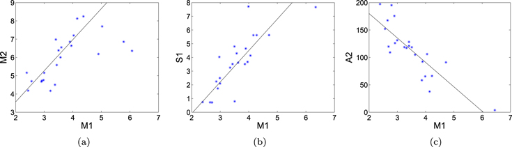
Figure 2. Correlations between parameters M1 and M2 (left panel), parameters S1 and M1 (middle panel), and parameters A2 and M1 (right panel).
Download figure:
Standard image High-resolution image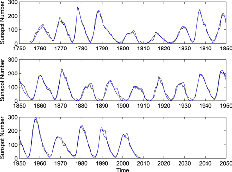
Figure 3. Monthly sunspot number (thin black line) and fitting curve (thin blue line) from the three-parameter function for cycles 1–23.
Download figure:
Standard image High-resolution imageTable 3. Best-fit Parameters for the Three-parameter Function and Some Measures of Goodness of Fit
| Cycle Number |

|

|

|

|

|
CC |
|---|---|---|---|---|---|---|
| 1 | 119.39 | 5.31 | 10.13 | 1.76 | 13.97 | 0.9501 |
| 2 | 49.00 | 2.52 | 8.88 | 1.28 | 11.95 | 0.9747 |
| 3 | 184.15 | 2.83 | 5.67 | 1.21 | 8.29 | 0.9948 |
| 4 | 153.10 | 3.44 | 21.56 | 1.04 | 8.55 | 0.9914 |
| 5 | 69.72 | 4.20 | 2.13 | 1.70 | 8.77 | 0.9666 |
| 6 | 66.06 | 5.83 | 14.07 | 2.55 | 8.32 | 0.9546 |
| 7 | 122.48 | 6.19 | 2.10 | 0.76 | 6.78 | 0.9877 |
| 8 | 156.51 | 2.97 | 8.27 | 0.61 | 6.41 | 0.9960 |
| 9 | 184.67 | 4.98 | 14.84 | 1.78 | 18.76 | 0.9645 |
| 10 | 126.75 | 3.86 | 13.17 | 0.94 | 6.88 | 0.9931 |
| 11 | 171.38 | 3.28 | 5.33 | 1.46 | 10.77 | 0.9892 |
| 12 | 101.59 | 3.48 | 2.00 | 1.91 | 13.72 | 0.9699 |
| 13 | 147.42 | 4.49 | 1.13 | 2.92 | 16.86 | 0.9378 |
| 14 | 105.33 | 4.34 | 2.16 | 1.08 | 6.21 | 0.9844 |
| 15 | 161.09 | 4.53 | 0.00 | 2.32 | 14.74 | 0.9678 |
| 16 | 115.82 | 3.40 | 2.14 | 2.44 | 13.89 | 0.9686 |
| 17 | 142.66 | 3.59 | 7.75 | 0.62 | 5.22 | 0.9964 |
| 18 | 183.46 | 3.47 | 5.99 | 1.41 | 10.97 | 0.9864 |
| 19 | 256.05 | 3.50 | 6.58 | 2.18 | 13.51 | 0.9904 |
| 20 | 65.95 | 3.18 | 13.72 | 1.61 | 8.69 | 0.9846 |
| 21 | 222.17 | 3.61 | 3.78 | 1.87 | 11.43 | 0.9927 |
| 22 | 126.31 | 2.65 | 7.76 | 1.75 | 15.62 | 0.9804 |
| 23 | 53.47 | 2.73 | 11.06 | 1.59 | 10.92 | 0.9863 |
| 1–23 | 1.64 | 11.83 | 0.9838 | |||
Download table as: ASCIITypeset image
3. COMPARISON OF FIT EFFECT FOR THE FIVE FUNCTIONS
Figure 1 shows five fitting curves by the quasi-Planck function (function-P), the binary mixture of Laplace functions (function-L), the one-parameter function from dynamo models (function-D), the modified Gaussian function (function-G), and the binary mixture of Gaussian functions (function-C), and the last one matches the best, as well as Figure 4.
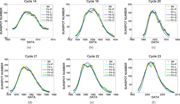
Figure 4. Comparisons between the five functions for six cycles with significant bimodal structure. Shown are the smoothed monthly sunspot number (circles) and its fit by the quasi-Planck function (cyan lines), the binary mixture of Laplace functions (yellow lines), the one-parameter function from dynamo models (blue lines), the modified Gaussian function (green lines), and the binary mixture of Gaussian functions (black lines) for (a–f) cycles 14, 16, 20, 21, 22, and 23.
Download figure:
Standard image High-resolution image3.1. Deviation
The fitting deviation (Li 1999) is measured by the following function:
where  is the smoothed monthly sunspot number,
  is the functional fit value, and
  is the number of months in the cycle. The fitting deviations about the proposed binary mixture of Gaussian functions for each cycles are listed in the ninth column of Table 1, and it is 6.54 computed for all 23 cycles. The fitting deviation for each of the 23 cycles by function-P, function-L, function-D, function-G, and function-C is shown in Figure 5(b), and Table 2 lists deviations computed for the overall cycles. It is obvious that function-C has the least deviation. The binary mixture of Gaussian functions gives a very perfect fit.
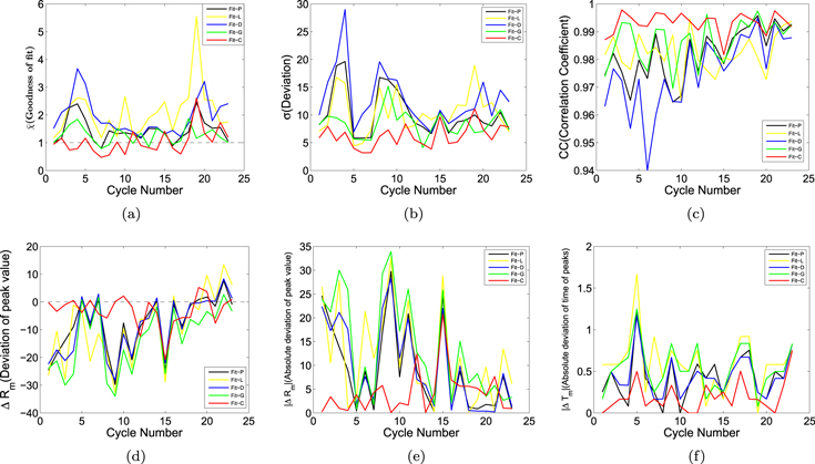
Figure 5. Comparisons of fitting effects (a)  , (b)
, (b)  , (c) CC, (d)
  , (e)
, (e)  , and (f)
  among the quasi-Planck function (black lines), the binary mixture of Laplace functions (yellow lines), the one-parameter function from dynamo models (blue lines), the modified Gaussian function (green lines), and the binary mixture of Gaussian functions (red lines).
Download figure:
Standard image High-resolution image3.2. Correlation Coefficient
The correlation coefficient (Bevington & Robinson 2003) is defined as follows:
where  is the smoothed monthly sunspot number,
  is the mean value of the data R,
  is the functional fit value, and
  is the number of months in the cycle. The correlation coefficients for each of the 23 cycles, between the data and the functional value, are listed in the 10th column of Table 1. It is 0.9838 when calculated for the whole duration, significant at the
  confidence level. The CC for fitting by the five functions mentioned above to all 23 cycles is listed in Table 2. Figure 5(c) shows the CC for fitting by the five functions mentioned above to each of the 23 cycles, and the red line shows that the fitting by the binary mixture Gaussian function is obviously closer to the horizontal line of value 1, indicating that function-C gives the best description on the whole.
3.3. Fitting Effect at Peaks
Cycles 14, 16, 20, 21, 22, and 23 clearly present a double-peak structure. Comparisons among the five functions for these cycles are shown in Figure 4. The binary mixture of Gaussian functions gives the best description of the cycles on the whole, but the binary mixture of Laplace distribution functions does better for those cycles that present a deep Gnevyshev gap. Peaks fitting with the modified binary mixture of Laplace distribution functions and the binary mixture of Gaussian functions are compared as an exception, and the latter is closer to the smoothed sunspot number curve, as shown in Figure 6.

Figure 6. Comparison of fitting results at peaks. The blue line is the smoothed monthly sunspot number, and the black asterisks are the peaks of the fitting curves with the modified binary mixture of Laplace distribution functions (Sabarinath & Anilkumar 2008), which are obviously higher than the actual peaks of the observation data. The red asterisks are the peaks of the fitting curves with the binary mixture of Gaussian functions, which are almost superpositions to the actual peaks of the observation data.
Download figure:
Standard image High-resolution imageThe average difference ( ) of peak values among all 23 cycles is computed as

where Rm is the fitting peak value and Am is the observed peak value. The averages by the quasi-Planck function ( ), the binary mixture of Laplace functions (
 ), the one-parameter function from dynamo models (
 ), the modified Gaussian function (
 ), and the binary mixture of Gaussian functions (
 ) are given in Table 2. On average, the fitting peak sizes by the Planck function, one-parameter function, and Gaussian function are smaller than observations, while those by the binary mixture of Laplace distribution functions are much greater than their corresponding observational peaks (see Figures 1 and 6). The fitting peak sizes by the binary mixture of Gaussian functions are also smaller than the observed ones on average, but not as much as by function-P, function-D, or function-G.
The average absolute differences for peak values between the fit values and the observed values

are also given in Table 2, by the five fitting functions-P, L, D, G, and C ( ,
,  ,
,  ,
,  ,
,  ). Of these five functions, the binary mixture of Gaussian functions provides functional peak values with the least average absolute deviation (
 ) from the observations.
The average absolute difference ( ) for peak timings between the fit values (
 ) and the observed values (
 ) is given as

The average absolute differences by the five fitting functions mentioned before ( ,
,  ,
,  ,
,  ,
,  ) are given in Table 2. Of these five fitting functions, the binary mixture of Gaussian functions provides the functional peak timings with the least average absolute deviation (
 ) from the observations. Comparisons of
  ,
,  , and
, and  among the five functions are shown in Figures 5(d)–(f), respectively.
4. FEATURES OF SUNSPOT CYCLES
4.1. Amplitude versus Period
Features of sunspot cycles were investigated according to the fitting results by the binary mixture of Gaussian functions. The correlation coefficient between amplitude ( ) and period (
 ) from the same cycle is only −0.2930, statistically insignificant. But there is a strong correlation between the amplitude (
 ) and the length of the previous cycle (
 ), shown in Figure 7. The thin line in the figure is the regression line of the equation

with a correlation coefficient  , significant at the
  confidence level. The figure shows that the shorter the period of a cycle is, the larger the amplitude of its following cycle is. In other words, a short cycle should generally follow a strong activity cycle, the same trend as what Carrasco et al. (2016) gets from the new sunspot number index.
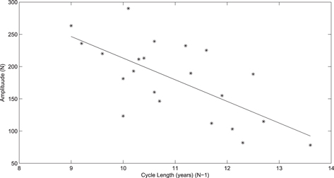
Figure 7. Relationship of the amplitude Rm and the length of the previous cycle ( ). The thin line is the regression line, showing a negative correlation.
Download figure:
Standard image High-resolution image4.2. Amplitude versus Rise Time
Correlation between the rise time (Trise) and the amplitude (Rm) is shown in Figure 8. The regression line in the figure is

and the regression coefficient  , significant at the
  confidence level. Though Carrasco et al. (2016) used a different linear equation to describe the relationship between amplitude and rise time, the inverse proportional function gives the same result as negative correlation. The time taken for the sunspot number to rise to maximum is inversely correlated to the cycle amplitude, which is the so-called Waldmeier effect (Waldmeier 1935, 1939).

Figure 8. Correlation between the rise time and the amplitude. The thin curve is the regression line, which shows a downward trend.
Download figure:
Standard image High-resolution image4.3. Amplitude versus Asymmetry
Figure 9 shows a correlation between asymmetry (c) and the amplitude (Rm). The thin line in this figure shows an upward trend, in the form of

where c presents asymmetry, the ratio of the decline time (Tdecline) to the rise time (Trise) (Li et al. 2009). That is to say, cycles with larger amplitude are more asymmetric. The correlation coefficient is 0.6884, significant at the  confidence level.
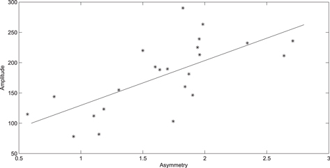
Figure 9. Relation between asymmetry and the amplitude. The linear regression line shows an upward trend, representing a positive correlation.
Download figure:
Standard image High-resolution image4.4. Even–Odd Effect
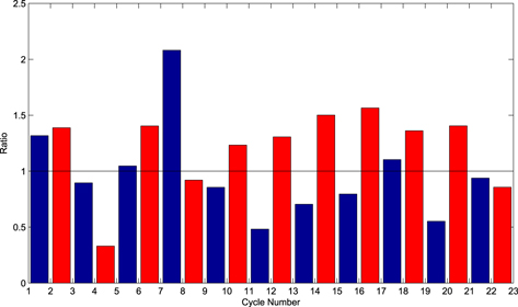
The ratios of the odd-cycle amplitude ( ) to the preceding even-cycle amplitude (
 ) are shown in Figure 10 as red bars:

For 8 of the total 11 paired cycles, the ratio is greater than 1. The ratios are about 1.21 on average. A ratio greater than 1 means that the odd-cycle amplitude is greater than the preceding even-cycle amplitude. The ratios of the even-cycle amplitude ( ) to the preceding odd-cycle amplitude (
 ) are also shown in the figure as blue bars:

For 7 of the total 11 paired cycles, the ratio is less than 1. The ratios are 0.98 on average. Thus, there is a noticeable feature when  is compared with
  , which is the so-called Gnevyshev–Ohl rule or Even–Odd effect (Gnevyshev & Ohl 1948).
Figure 10. Red bars show the ratio of the odd-cycle amplitude to the preceding even-cycle amplitude. Blue bars show the ratio of the even-cycle amplitude to the preceding odd-cycle amplitude.
Download figure:
Standard image High-resolution image
5. CONCLUSION
Dates of the 13-month smoothed monthly sunspot number (cycles 1–23) from the new version of sunspot number issued by the SIDC are used to discuss the shape of the solar cycles. Most of the time, the shape of sunspot cycles has been studied with single-peak functions. But in fact, the shape of sunspot cycles is more complicated than such a single-peak flowing curve. And a lot of research said that the shape of the sunspot cycle is a double-peak curve. A functional form using a binary mixture of Gaussian functions has been used here to study the shape of the sunspot cycle,

that could behave as a double-peak shape. The best-fit parameters for cycles 1–23 are computed by using the least-squares method. Examinations of the goodness of fit show that the binary mixture of Gaussian functions passes within 1.09 standard deviations of the actual data, extremely near to 1. The fitting deviation by the proposed binary mixture of Gaussian functions is 6.54. The correlation coefficient between the functional values and the smoothed monthly sunspot number is 0.9948, significant at the  confidence level. The above examinations explain that the binary mixture of Gaussian functions gives a very perfect fit of cycle shape. The fitting effects at peaks are also investigated. Fitting with the binary mixture of Gaussian functions, the functional peak values have the absolute deviation,
  , from the observations, and the functional peak timings have the average absolute deviation,
  , from the observed ones. Even after reducing the number of free parameters to 3, it could also adequately reproduce the shape,

with a correlation coefficient of 0.9838, significant at the  confidence level. Features of the sunspot cycle shape are inspected based on the fitting by the binary mixture of Gaussian functions. They have the same trends and approximate correlation coefficients when comparing to what Carrasco et al. (2016) obtained from the new sunspot number index. That is to say, the function keeps the solar-cycle characteristics well. The shape of the sunspot cycle is generally asymmetric, taking more time declining to the next minimum from the maximum than rising from the starting minimum to the maximum. And cycles with larger amplitude are more asymmetric. The larger the amplitude is, the shorter the period is. The time taken for the sunspot number to rise to maximum is inversely related to the cycle amplitude, like the Waldmeier effect. The odd-cycle amplitude is generally greater than the preceding even-cycle amplitude, with an average ratio of 1.21, which is the so-called Even–Odd effect.
The authors are much indebted to Ke-Jun Li for his constructive proposals and helpful suggestions. This work is supported by the National Natural Science Foundation of China (11573065, 11633008, 11273057, 11603071, and 11603069), the Specialized Research Fund for State Key Laboratories, and the Chinese Academy of Sciences.
The authors declare that they have no conflicts of interest.