Polarization of Coronal Forbidden Lines

The magnetic field, which dominates the dynamics and topology of most coronal phenomena, is indeed the key parameter to understand how the solar corona is heated, how the mass and energy are transported, how the solar wind is accelerated, and how the eruptive phenomena are generated (Aschwanden 2005). However, the diagnostics of the magnetic field in the solar corona still faces challenges, simply because the coronal plasma is optically thin and the magnetic field is intrinsically weak (usually less than 10 G). During the past decades, with the help of the quantum theory of matter–radiation interaction in the density matrix formalism, methods to diagnose the vector magnetic field in the solar corona have been developed, leading to the measurement of the magnetic field vector in solar prominences by means of linear polarization observation (Bommier & Sahal-Brechot 1978; Bommier et al. 1981; Landi Degl'Innocenti 1982). Although the Zeeman effect still remains the most reliable method for the diagnostics of solar magnetic fields, an alternative technique, based on the observation of the linear polarization in forbidden coronal lines, has recently been developed (Raouafi 2011; Capobianco et al. 2014; Trujillo Bueno 2014). In the solar corona, anisotropic illumination leads to population imbalances among the sublevels of the ions. This phenomenon, called optical pumping, is responsible for the polarization of radiation. The differences in population among the ionic sublevels are modified by the magnetic field through the Hanle effect  (Stenflo 1994; Landi Degl'Innocenti & Landolfi 2004), where the information is encoded on the magnetic field. In contrast to the Zeeman effect, the Hanle effect is sensitive to weak magnetic fields and only exists in situations of non-local thermodynamic equilibrium (Landi Degl'Innocenti 2001). Due to the low values of the Einstein coefficients for magnetic dipole transitions, the Hanle effect is saturated even for magnetic fields as low as 10⁻⁴ G, a value smaller than the typical field intensity in the corona. This means that the linear polarization of forbidden coronal lines is not sensitive to the intensity, but only to the orientation of the magnetic field. For diagnostic purposes, only the direction of the magnetic field projected on the plane of sky can be determined, and such direction is either perpendicular or parallel to the orientation of the linear polarization.

In this paper, we mainly focus on the coronal forbidden (magnetic dipole transition) line polarimetry technique (Judge 1998; Judge et al. 2013), which was first suggested by Charvin (1965). More detailed theoretical contributions were later provided by Hyder (1965), House (1974), House et al. (1982), Casini & Judge (1999), and Lin & Casini (2000) using both quantum and classical theories. The collision effects on the polarization of the green line (Fe xiv 5303 Å) and the infrared line (Fe xiii 10747 Å) were investigated by Sahal-Brechot (1974a, 1974b, 1977) and House (1977). By applying a synthesis code developed by Judge & Casini (2001), Judge et al. (2006) showed that the linear polarization of forbidden lines is capable of tracing current sheets in the solar corona.

Observational efforts on the same theme have been carried out by Eddy & McKim Malville (1967), Mickey (1973), Arnaud (1982a, 1982b), Arnaud & Newkirk (1987), Querfeld (1982), Querfeld & Smartt (1984), and Tomczyk et al. (2007), who showed the feasibility of measuring the direction of the coronal magnetic fields by linear polarization. Liu & Lin (2008) compared the observed and synthesized polarization of the Fe xiii 10747 Å line by using a potential coronal magnetic field model and showed that the simulations are consistent with observations. More recent observations carried out with the Coronal Multi-channel Polarimeter (Tomczyk et al. 2008) and relative simulations by Dove et al. (2011) and Ba̧k-Stȩślicka et al. (2013) have shown that the linear polarization of the Fe xiii 10747 Å line is capable of tracing prominence cavities. In contrast to the linear polarization, observations of circular polarization have seldom been performed. Harvey (1969) and Kuhn & Penn (1995) attempted to use the circular polarization of the Fe xiv 5303 Å and Fe xiii 10747 Å lines to measure the coronal magnetic field intensity and set an upper limit of 40 G on the field intensity above active regions. More accurate observations in the Fe xiii 10747 Å line have been achieved by Lin et al. (2004), who proved the possibility of observing the Zeeman effect in the corona. Qu et al. (2013, 2017) performed spectro-polarimetry observations during a total solar eclipse. Inversion techniques for the coronal magnetic field are still in a very preliminary phase. Studies of vector tomography for the coronal magnetic field have been made by Kramar et al. (2006, 2013). Plowman (2014) employed a Markov Chain Monte Carlo search to infer the coronal magnetic field at a single point. Moreover, a toolset named FORWARD, developed by Gibson et al. (2016), can be applied to synthesize a broad range of coronal observations.

The aim of this paper is to investigate the linear polarization of coronal forbidden lines as a tool for diagnosing the magnetic field in the solar corona. The present article is organized as follows. In Section 2, we briefly outline the theory of the polarization of coronal forbidden lines in the density matrix representation (Casini & Judge 1999; Landi Degl'Innocenti & Landolfi 2004). The theory is then applied to synthesize the emergent polarization maps of the coronal forbidden lines. In Section 3, the influence of electronic collisions, active regions, and Thomson scattering on linear polarization is also examined in potential-field source-surface (PFSS) coronal magnetic field models. The long-term evolution of the magnetic field in the solar corona is discussed in Section 3.3 via the forbidden line polarimetry technique. Finally, the main properties of the linear polarization of the coronal forbidden line technique are summarized in Section 4.

The quantum theory of spectral line polarization that is adopted in this paper was developed by Landi Degl'Innocenti (1983, 1984, 1985) in the framework of the density matrix formalism. It is assumed that the radiation scattered by the ions in the corona is purely of photospheric origin. Since the coronal forbidden lines are not present in the photospheric spectrum and we explicitly rule out the possibility that strong photospheric lines may be shifted into the spectral range of the coronal lines because of bulk plasma motions, the so-called hypothesis of the flat-spectrum approximation is fully justified. Due to the large degree of ionization of the ions in the solar corona, fine structure intervals turn out to be very large, which ensures that quantum interference between different J-levels can safely be ignored. Consequently, such ions can be treated as multilevel atoms rather than multiterm atoms. Because the corona is optically thin, we perform an integration along the line of sight to take into account the contribution of all the volume elements that contribute to the observed radiation. In the following subsections, we briefly summarize the equations used in the simulation. Further details can be found in the monograph by Landi Degl'Innocenti & Landolfi (2004).

2.1. Density Matrix

When an atomic system is excited by anisotropic radiation, its magnetic sublevels are not equally populated and definite phase relations exist among them. This phenomenon is referred to as atomic polarization and can be suitably described using the concept of the atomic density matrix operator, which was introduced by Fano (1957) to describe in full generality the excitation states of the atomic system. In this representation, the diagonal matrix elements $\rho (\alpha {JM},\alpha {JM})$ represent the population of the atomic levels, and the off-diagonal matrix elements $\rho (\alpha {JM},\alpha ^{\prime} J^{\prime} M^{\prime} )$ describe the interference terms. We adopt the multipolar components of the atomic density matrix as defined in Omont (1977):

$$\begin{eqnarray}{\rho }_{Q}^{K}(J) & = & \displaystyle \sum _{{MM}^{\prime} }{(-1)}^{J-M}\sqrt{2K+1}\left(\begin{array}{ccc}J & J & K\\ M & -M^{\prime} & -Q\end{array}\right)\\ & & \times {\rho }_{J}(M,M^{\prime} ),\end{eqnarray} \tag{ 1 }$$

where K = 0, 1,..., 2J, Q = −K, −K + 1,..., K − 1, K, and where the expression in brackets is the Wigner 3j symbol. In terms of the density matrix, $\sqrt{2J+1}\,{\rho }_{0}^{0}$ indicates the total population of the level, while the rank 1 and rank 2 tensorial components describe the orientation and alignment of the atomic level, and contribute respectively to the circular and linear polarization.

Due to the low values of the Einstein coefficients of the magnetic dipole transitions, the Hanle effect is saturated even for magnetic fields as weak as 10⁻⁴ G, which means that if one chooses the magnetic field direction as the quantization axis, the interference between magnetic sublevels can be ignored, and only the density matrix elements ${\rho }_{Q}^{K}(\alpha J)$ with Q = 0 are nonzero. However, for diagnostic purposes, this also implies that there is no possibility to measure the magnetic field strength from linear polarization observations in forbidden lines, since only the direction of the magnetic field affects the linear polarization.

2.2. Incident Radiation

The incident radiation scattered by the ions in the corona essentially comes from the photosphere, and for the purpose of this work, it is assumed that it has no spectral structure across the wavelength interval covered by the forbidden line. This allows the flat-spectrum approximation to be used, and moreover, implies that the radiation field incident on the ions does not depend on the velocity of the ion, either due to the solar wind or to thermal effects. The incident radiation field can then be described by a unique irreducible tensor (Landi Degl'Innocenti 1983),

$$\begin{eqnarray}&&{J}_{Q}^{K}(\nu )=\int \displaystyle \frac{d{\rm{\Omega }}}{4\pi }\displaystyle \sum _{i=0}^{3}{{ \mathcal T }}_{Q}^{K}(i,{\rm{\Omega }}){S}_{i}(\nu ,{\rm{\Omega }}),\end{eqnarray} \tag{ 2 }$$

where ${S}_{i}(\nu ,{\rm{\Omega }})=I,Q,U,V$ denotes the intensity in the four Stokes parameters and ${{ \mathcal T }}_{Q}^{K}(i,{\rm{\Omega }})$ is the irreducible spherical tensor of the polarization unit vectors, which specifies the geometry of the incident radiation (Landi Degl'Innocenti 1984). Assuming that the incident radiation is unpolarized, and ignoring the presence of active regions, the radiation field is cylindrically symmetric in the reference system with the z-axis directed along the solar radius, and can be fully described by only two components ${J}_{0}^{0}(\nu )$ and ${J}_{0}^{2}(\nu )$ of the radiation field tensors, or alternatively, by the component ${J}_{0}^{0}(\nu )$ and the anisotropy factor w_ν:

$$\begin{eqnarray}{J}_{0}^{0}(\nu ) & = & \oint \displaystyle \frac{d{\rm{\Omega }}}{4\pi }I(\nu ,\mu ),\\ {J}_{0}^{2}(\nu ) & = & \displaystyle \frac{1}{2\sqrt{2}}\oint \displaystyle \frac{d{\rm{\Omega }}}{4\pi }(3{\mu }^{2}-1)I(\nu ,\mu ),\\ {w}_{\nu } & = & \sqrt{2}\displaystyle \frac{{J}_{0}^{2}(\nu )}{{J}_{0}^{0}(\nu )},\end{eqnarray} \tag{ 3 }$$

where $I(\nu ,\mu )$ is the intensity of the incident radiation and $\mu =\cos \theta$, with θ the heliocentric angle. In this equation, ${J}_{0}^{0}(\nu )$, the radiation field tensor of rank 0, indicates the mean intensity of the incident radiation, and the atomic polarization results from the term ${J}_{0}^{2}(\nu )$, which describes the anisotropy of the radiation. Obviously, the component ${J}_{0}^{2}(\nu )$ and the factor w_ν are zero if the radiation field is isotropic. When the incident radiation is unpolarized, the incident radiation tensors of rank 1 are zero, which implies that the density matrix elements ${\rho }_{Q}^{K}(\alpha J)$ with K = 1 are all zero.

Figure 1 describes the behavior of w_ν as a function of the distance R from the solar disk center. The coefficients of limb darkening are taken from Allen (1973). As seen in Figure 1, the anisotropy factor w_ν increases with height for the visible and infrared lines, and for any given height, the shorter the wavelength is, the larger is the anisotropy factor for the spectral range covered by Allen's relations. The difference between the anisotropy factors relative to the various wavelengths becomes negligible at higher layers.

Zoom In Zoom Out Reset image size

2.3. Emission Coefficients

To simulate imaging polarimetric observations, it is convenient to neglect the spectral details of the line and to consider the frequency-integrated emission coefficients,

$$\begin{eqnarray}&&{\tilde{\varepsilon }}_{i}({\boldsymbol{\Omega }})={\int }_{{\rm{\Delta }}\nu }{\varepsilon }_{i}(\nu ,{\boldsymbol{\Omega }})d\nu ,\end{eqnarray} \tag{ 4 }$$

where ${\varepsilon }_{i}(\nu ,{\boldsymbol{\Omega }})$ is the emission coefficient in the ith Stokes parameter and the interval ${\rm{\Delta }}\nu$ is sufficiently broad to fully cover all the Zeeman components of the line and shifts due to the Doppler effect. The frequency-integrated emission coefficients in the Stokes parameters are given by (Landi Degl'Innocenti 1984)

$$\begin{eqnarray}{\tilde{\varepsilon }}_{i}({\boldsymbol{\Omega }}) & = & \displaystyle \frac{h\nu }{4\pi }{ \mathcal N }\sqrt{2{J}_{u}+1}A({\alpha }_{u}{J}_{u}\to {\alpha }_{{\ell }}{J}_{{\ell }})\\ & & \times \displaystyle \sum _{{KQ}}{w}_{{J}_{u}{J}_{{\ell }}}^{(K)}{{ \mathcal T }}_{Q}^{K}(i,{\boldsymbol{\Omega }}){\rho }_{Q}^{K}({\alpha }_{u}{J}_{u}),\end{eqnarray} \tag{ 5 }$$

where ${ \mathcal N }$ is the ion density and ${w}_{{J}_{u}{J}_{{\ell }}}^{(K)}$ is a numerical factor depending on J_u and ${J}_{{\ell }}$, the angular momenta of the upper and the lower levels of the transition, respectively. It is noteworthy that the geometrical tensors ${{ \mathcal T }}_{Q}^{K}(i,{\boldsymbol{\Omega }})$ for the electric dipole transitions are distinct from those for the magnetic dipole transitions. Due to the character of the magnetic dipole transition, ${{ \mathcal T }}_{Q}^{K}{(i,{\boldsymbol{\Omega }})}_{M1}$ and ${{ \mathcal T }}_{Q}^{K}{(i,{\boldsymbol{\Omega }})}_{E1}$ are related by (Casini & Judge 1999)

$$\begin{eqnarray}&&{{ \mathcal T }}_{Q}^{K}{(i,{\boldsymbol{\Omega }})}_{M1}=\left\{\begin{array}{r}{{ \mathcal T }}_{Q}^{K}{(i,{\boldsymbol{\Omega }})}_{E1},(i=0,3)\\ -{{ \mathcal T }}_{Q}^{K}{(i,{\boldsymbol{\Omega }})}_{E1},(i=1,2)\end{array}\right.,\end{eqnarray} \tag{ 6 }$$

where E1 and M1 denote the electric and magnetic dipole transitions, respectively.

In terms of the emission coefficients, ${\tilde{\varepsilon }}_{2}({\boldsymbol{\Omega }})$ is zero if the reference direction of Stokes Q is either parallel or perpendicular to the magnetic field direction projected on the plane of sky, which also indicates that the orientation of the linearly polarized emission is either parallel or perpendicular to the projection of the magnetic field vector, and it totally depends on the sign of ${\rho }_{0}^{2}({\alpha }_{u}{J}_{u})$. In the synthesis code, a reference system with the z-axis directed along the solar radius is adopted to calculate the incident radiation tensors according to Equation (3). Then, the incident radiation tensors are transformed to the reference of the magnetic field via Euler rotations, which are performed by using the quantum angular momentum rotation matrices of order K = 0–2. In the reference of the magnetic field, the statistical equilibrium equations have a simpler form for the forbidden lines. Only the density matrix elements ${\rho }_{Q}^{K}(\alpha J)$ with K even and Q = 0 are present in the equations. To obtain the emergent emission signal, we perform an integration to take into account the contribution from all the particles along the line of sight, due to the fact that the corona is optically thin.

2.4. Coronal Model

We adopt a one-dimensional spherically symmetric coronal model giving temperature and proton density as a function of distance from the solar disk center (Wang et al. 1993). This is the same model as that used by Khan et al. (2011) to simulate the linear polarization of hydrogen Lyα. The model is shown in Figure 2. Assuming that hydrogen and helium are totally ionized in the corona, the proton density is related to the electron density by a factor ${N}_{p}/{N}_{e}=0.83$. We write the ion density using the following expression,

$$\begin{eqnarray}&&N({{\rm{X}}}^{+m})=\displaystyle \frac{N({{\rm{X}}}^{+m})}{N({\rm{X}})}\displaystyle \frac{N({\rm{X}})}{N({\rm{H}})}N({\rm{H}}),\end{eqnarray} \tag{ 7 }$$

where $N({{\rm{X}}}^{+m})/N({\rm{X}})$ denotes the ionization fraction of element X, which is taken from the CHIANTI database, and $N({\rm{X}})/N({\rm{H}})$ is the abundance ratio of the element X with respect to hydrogen in the solar corona according to Schmelz et al. (2012).

Zoom In Zoom Out Reset image size

The basic data concerning various coronal forbidden lines are listed in Table 1. The Einstein coefficients for spontaneous de-excitation, according to the NIST (National Institute of Standards and Technology) database, are listed in the second column (Kramida et al. 2015). Although the Einstein coefficients for the Si x 14300 Å, Mg viii 30280 Å, and Si ix 39290 Å lines are much smaller than those of the visible lines, the corresponding scattering cross-sections turn out to be comparable. The frequency-integrated absorption cross-section of an atomic transition (which coincides with the scattering cross-section in the absence of collisions) is given by Landi Degl'Innocenti (2014):

$$\begin{eqnarray}&&{\tilde{\sigma }}_{A}=\displaystyle \frac{\pi {e}_{0}^{2}}{{mc}}f,\end{eqnarray} \tag{ 8 }$$

where e₀ is the electron charge, m is the electron mass, and c is the velocity of light. The oscillator strength f is connected to the Einstein coefficient by

$$\begin{eqnarray}&&f=\displaystyle \frac{{{mc}}^{3}}{8{\pi }^{2}{e}_{0}^{2}{\nu }_{{ab}}^{2}}\displaystyle \frac{{g}_{a}}{{g}_{b}}{A}_{{ab}}.\end{eqnarray} \tag{ 9 }$$

where ${\nu }_{{ab}}$ and A_ab are the frequency and Einstein coefficient of the transition, respectively, and g_a and g_b are the statistical weights of the upper and the lower level, respectively. The oscillator strengths of the forbidden lines are listed in the fourth column. Apart from the scattering cross-section, the emission in the forbidden line depends on several factors, namely the intensity of the incident radiation (the incident radiation is weaker in the infrared band than in the visible band), the elemental abundance, and the ionization fraction of the element (which is a function of temperature). The elemental abundance and the temperature for which the ionization fraction is maximum are listed in the fifth and sixth columns. The seventh column lists the numerical factor ${W}_{2}({J}_{{\ell }},{J}_{u})$, which is proportional to the fractional polarization of the emission. The Fe xi 7982 Å line is a transition line with J_u = 1 and ${J}_{{\ell }}=2$, and the corresponding ${W}_{2}({J}_{{\ell }},{J}_{u})$ factor is only 0.01, which means that the linear polarization will be very weak. The upper level of the red line (Fe x 6374 Å) has ${J}_{u}=1/2$ and ${W}_{2}({J}_{{\ell }},{J}_{u})$ turns out to be zero. In principle, no linear polarization can thus be expected in this line. For the lines Fe xiii 10747 Å and Si ix 39290 Å, whose ${W}_{2}({J}_{{\ell }},{J}_{u})$ is 1, a large degree of linear polarization should be expected.

Table 1.  Atomic Information of Several Coronal Forbidden Lines

	Auℓ $({s}^{-1})$	${J}_{u}\to {J}_{{\ell }}$	f	Abundance	$\mathrm{log}\,{T}_{\max }$	${W}_{2}({J}_{{\ell }},{J}_{u})$
Fe xiv 5303 Å	60.2	$\tfrac{3}{2}\to \tfrac{1}{2}$	$5.08\times {10}^{-7}$	$7.08\times {10}^{-5}$	6.29	0.5
Fe x 6374 Å	69.4	$\tfrac{1}{2}\to \tfrac{3}{2}$	$3.24\times {10}^{-7}$	$7.08\times {10}^{-5}$	6.04	0
Fe xi 7892 Å	43.7	1 → 2	$2.45\times {10}^{-7}$	$7.08\times {10}^{-5}$	6.13	0.01
Fe xiii 10747 Å	14.0	1 → 0	$7.27\times {10}^{-7}$	$7.08\times {10}^{-5}$	6.25	1
Si x 14300 Å	2.69	$\tfrac{3}{2}\to \tfrac{1}{2}$	$1.65\times {10}^{-7}$	$7.24\times {10}^{-5}$	6.15	0.5
Mg viii 30280 Å	0.323	$\tfrac{3}{2}\to \tfrac{1}{2}$	$8.88\times {10}^{-8}$	$7.41\times {10}^{-5}$	5.91	0.5
Si ix 39290 Å	0.289	1 → 0	$2.01\times {10}^{-7}$	$7.24\times {10}^{-5}$	6.05	1

Note. The coronal elemental abundances are given by Schmelz et al. (2012). The value of ${T}_{\max }$ is the temperature of the maximum ionization fraction according to the CHIANTI database. The factor ${W}_{2}({J}_{{\ell }},{J}_{u})$ is defined by Landi Degl'Innocenti & Landolfi (2004).

Download table as:  ASCIITypeset image

A synthetic map of the fractional linear polarization $\sqrt{{Q}^{2}+{U}^{2}}/I$ of the green line in the absence of magnetic field is presented in Figure 3. To perform the simulation, we have employed a 15 level atomic model of the Fe xiv ion. Actually, the difference between using a 15 level atomic model and a much simpler two-level atomic model is only about 1% in the degree of linear polarization. Due to the fact that the collisional excitation rates are comparable to the radiative excitation rates for the coronal forbidden lines, collisional transitions are taken into account in the statistical equilibrium equations. The transition rates are taken from the extended tables of Aggarwal & Keenan (2014). The multipole components of the collisional transition rates are calculated according to Landi Degl'Innocenti & Landolfi (2004), by assuming that collisional transitions are only due to the dipolar component of the atom–electron interaction. The figure shows that the degree of linear polarization increases with height and reaches a maximum value of 31.2% at the height of about 1 R_☉ over the solar surface. The direction of linear polarization is everywhere along the radius. This behavior is typical of lines due to magnetic dipole transitions (assuming that the anisotropy factor is positive). Electric dipole transitions would produce linear polarization parallel to the solar limb. This fact is due to the sign difference in the geometrical tensor, as shown in Equation (6). It is noteworthy that although the degree of polarization is an increasing function of height, the intensity, being proportional to the ion density, decreases with height. This makes the observation in the outer corona more difficult.

Zoom In Zoom Out Reset image size

Other synthetic maps of the green line polarization are shown in Figure 4. These maps are obtained for a dipolar magnetic field model, a typical configuration in the solar corona. The reference direction for positive Q is the S−N direction in the maps. Figures 4(a) and (b) are the color images of Stokes Q/I and U/I, respectively. The maximum (and minimum) values of Q/I are always located where U/I is equal to zero, and vice versa. The map of the fractional linear polarization is illustrated in Figure 4(c). In contrast to the non-magnetic situation, the maximum degree of linear polarization reduces to 22%, and some regions in the map turn out to be unpolarized. In Figure 4(d), we display the tilt angle (measured counterclockwise) of the linear polarization direction with respect to the direction of the non-magnetic case, i.e., with respect to the radial direction. In this map, the angle ranges from about −54° to 54°, and shows features similar to those of Figure 4(c). The rotation of linear polarization is a consequence of the presence of the magnetic field. In the polar region, the linear polarization is parallel to the direction of the magnetic field, and the tilt angle increases with the decrease of latitude until the linear polarization reaches zero. Then the angle decreases, and the linear polarization becomes perpendicular to the direction of the magnetic field in the equatorial region. This phenomenon is called the van Vleck effect. The linear polarization goes to zero in the regions where the angle ${\theta }_{B}$ between the magnetic field and the radial direction satisfies $3{\cos }^{2}{\theta }_{B}=1$, and the angle ${\theta }_{V}=\arccos (\sqrt{3}/3)=54\buildrel{\circ}\over{.} 7$ is called the van Vleck angle. This effect is related to the fact that the atomic alignment ${\rho }_{0}^{2}$ vanishes when $3{\cos }^{2}{\theta }_{B}=1$ in a cylindrically symmetric incident radiation field. When ${\theta }_{B}\lt {\theta }_{V}$, the sign of the atomic alignment ${\rho }_{0}^{2}$ coincides with that of the anisotropy factor, and the linear polarization is always parallel to the magnetic field direction as the anisotropy factor is positive in most situations. Conversely, when ${\theta }_{B}\gt {\theta }_{V}$, the sign of the atomic alignment ${\rho }_{0}^{2}$ will change, and the linear polarization will be perpendicular to the magnetic field direction. It is noteworthy to remark that in most situations, the tilt angle is less than $54\buildrel{\circ}\over{.} 7$, except when the magnetic field has a small inclination to the line of sight. When the magnetic field is almost pointing toward to the observer, the projection of the magnetic field direction on plane of the sky can take any value. The direction of linear polarization is also arbitrary in the plane of sky. However, in this situation, the signal of linear polarization is weak and hard to detect after the line-of-sight integration.

Zoom In Zoom Out Reset image size

3.1. Polarization Maps for Magnetic Field Models Representative of the Solar Minimum and Maximum

To investigate the long-term variation of the emergent polarization signals in the solar corona, we employ PFSS coronal magnetic field models (Schatten et al. 1969; Hoeksema 1984) provided by the Wilcox Solar Observatory (WSO) team. The PFSS model, which assumes that the global large-scale magnetic field is a potential in the corona, is basically an extrapolation of the photospheric magnetic field, measured by magnetographs, to the corona. These models are capable of reproducing the basic structure of the coronal magnetic field. Although the WSO data have a rather low spatial resolution, the WSO telescope has been in operation continuously since 1976, and it is suitable for investigating the long-term global magnetic field evolution. In the simulation, we adopted magnetic field models resulting in the development of associated spherical harmonics up to the 29th order. Figure 5 presents the hairy-ball plots of the PFSS coronal magnetic field models based on WSO data corresponding to Carrington rotations CR2055 and CR2122. The black curves depict closed magnetic field lines while the red and green curves depict open magnetic field lines of negative and positive polarities, respectively. The left panel in Figure 5 shows a dipolar configuration representative of solar minimum conditions, while the right panel is representative of solar maximum conditions, and shows a much more complex configuration. The PFSS models may miss some small structures in the corona. However, the loop-like structure can clearly be seen in the plots, and the models are capable of reproducing the large global magnetic field structure, which makes them suitable for our research.

Zoom In Zoom Out Reset image size

Synthetic polarization maps corresponding to CR2055 are shown in Figures 6(a) and (b), top panels, where loop-like structures can clearly be seen. In the polar regions, where the magnetic field is open, the direction of linear polarization is always along the solar radius. In general, considering a single point in the map, the direction of the magnetic field cannot be determined, due to the $90^\circ$ ambiguity. However, this ambiguity can be removed when the locations of the van Vleck null regions (unpolarized regions) can be identified on the map. These null regions are always located where the tilt angle has a discontinuity.

Zoom In Zoom Out Reset image size

If we assume that the magnetic field is smooth and continuous, the tilt-angle map can also provide information about the inclination of the magnetic field with respect to the plane of the sky. The geometry of the problem is presented in Figure 7. Near the van Vleck regions, the angle between the magnetic field and the radius direction is around ${\theta }_{V}=54\buildrel{\circ}\over{.} 7$. ${\theta }_{D}$ is the tilt angle on one side of the van Vleck null region, where the linear polarization is parallel to the magnetic field. The inclination ${\theta }_{I}$ between the magnetic field and the plane of sky can be roughly estimated by

$$\begin{eqnarray}&&\cos ({\theta }_{I})=\cos ({\theta }_{V})/\cos ({\theta }_{D}).\end{eqnarray} \tag{ 10 }$$

When ${\theta }_{D}={\theta }_{V}$, one gets ${\theta }_{I}=0^\circ$, and the coronal loops will be in the plane of sky. For the loop on the top-left corner of the map corresponding to CR2055, the tilt angle is about 52°, and the inclination of the field vector is about 20°. The bottom panels of Figure 6  illustrate the polarization maps of the solar maximum corresponding to CR2122. These maps show a much more intricate structure, especially in the north pole region. The intricate feature at the north pole implies that the magnetic field has a complex configuration. In contrast, the polarization is directed along the radius in the south pole region and shows that the magnetic field is open. This may indicate that the north pole is undergoing a polarity reversal, while the south pole is not. The polarity reversal will be discussed in detail in the next section. Furthermore, the tilt angle ranges from about −44° to 40°. We can also estimate that the inclination of the magnetic field on the bottom-left corner is about 36°. All the lines listed in Table 1, except Fe x 6374 Å, present the same tilt angle.

Zoom In Zoom Out Reset image size

3.2. Further Effects Influencing the Observed Polarization

The theoretical results obtained in the former sections are based on a series of hypotheses, or approximations, that may often fail to be satisfied in the solar corona. In this subsection, we discuss some effects that are capable of altering in a significant way the polarization maps discussed above.

3.2.1. The Role of Collisions

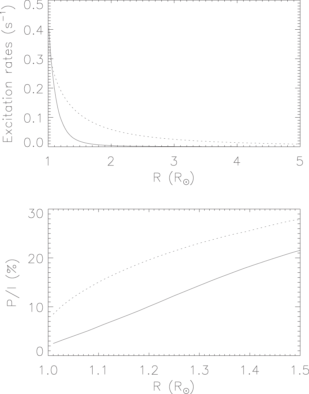
In the solar corona, the emissivity of the coronal forbidden lines is due to both resonance scattering and collisional excitation of the ions. Since the collisions are believed to be isotropic, ions excited by collisions cannot emit polarized radiation. The polarization of the forbidden line is thus caused only by the scattering of the anisotropic incident radiation. However, due to the fact that the Einstein coefficients for spontaneous de-excitation of forbidden transitions are small, the collisional excitation rates are in general comparable to the radiative excitations and have then to be included in the statistical equilibrium equations, as we have done using the collisional rates provided by Aggarwal & Keenan (2014). The main influence of collisions is obviously to reduce the degree of polarization. Sahal-Brechot (1974a, 1974b) found that the depolarization rates by proton impact are very weak, whereas the rates by electron impact are large enough to conspicuously reduce the degree of polarization. The top panel in Figure 8 shows the rates of collisional and radiative excitation in our present model. The collisions dominate the excitation of the coronal emission under a height of 0.1 solar radii above the solar surface. For larger heights, the collisional excitation rates diminish rapidly due to the decrease of electron density, and radiative excitation dominates. For heights above the solar surface larger than 1 R_☉, collisional excitations are so weak that they can be completely neglected. The bottom panel in Figure 8 shows the fractional linear polarization computed with and without collisional transitions, in the absence of magnetic field. In the figure, one can see that the collisions deeply reduce the amplitude of polarization. The collisions decrease the degree of linear polarization from 8% to 3% near the solar surface, and at a height of 0.5 R_☉, the linear polarization is reduced from 28% to 22%. This reduction effect due to collisions is large near the solar surface, where the electrons are denser, whereas in the higher layers the effect is much weaker.

Zoom In Zoom Out Reset image size

Figure 9 shows the synthetic polarization maps relative to the same magnetic field model as the one used in Figure 6, but in the absence of collisions. Compared to Figure 6, Figure 9 shows the same features, apart from a slight variation in the degree of polarization, which increase from about 27.2% to 29.9% for CR2055, and from about 20.8% to 22.8% for CR2122. In the tilt-angle maps, one can see that the direction of linear polarization is almost the same. The collisions mainly result in a decrease of the degree of maximum linear polarization, whereas the direction of linear polarization is not influenced since it only depends on the magnetic field orientation. This is important for diagnostic purposes, because the collisional rates are rather poorly known.

Zoom In Zoom Out Reset image size

3.2.2. Symmetry-breaking Effects

One challenging task of forbidden line polarimetry is to diagnose the magnetic field above active regions. This however raises a problem because the cylindrically symmetric hypothesis breaks down. Khan & Landi Degl'Innocenti (2011) and Khan et al. (2011) investigate the influence on linear polarization caused by the presence of an active region, and show how it can affect the amplitude and the direction of the linear polarization. In these cases, the radiation field can no longer be described in terms of the mean intensity and anisotropy factor alone. Further components of the radiation field tensor come into play. Supposing that the active region is seen under a small solid angle ${\rm{\Delta }}{\rm{\Omega }}$ from point P and that ${\rm{\Delta }}{I}_{\nu }$ is the intensity contrast with respect to the surrounding photosphere, the radiation field tensor at point P is given by

$$\begin{eqnarray}{J}_{0}^{0}(\nu ) & = & {[{J}_{0}^{0}(\nu )]}_{\mathrm{cyl}.{\rm{s}}.}+\displaystyle \frac{{\rm{\Delta }}{\rm{\Omega }}}{4\pi }{\rm{\Delta }}{I}_{\nu },\\ {J}_{0}^{2}(\nu ) & = & {[{J}_{0}^{2}(\nu )]}_{\mathrm{cyl}.{\rm{s}}.}+\displaystyle \frac{1}{2\sqrt{2}}(3{\cos }^{2}{\theta }_{0}-1)\displaystyle \frac{{\rm{\Delta }}{\rm{\Omega }}}{4\pi }{\rm{\Delta }}{I}_{\nu },\\ {J}_{\pm }^{2}1(\nu ) & = & \mp \,\displaystyle \frac{\sqrt{3}}{2}\sin {\theta }_{0}\cos {\theta }_{0}{e}^{\pm {\rm{i}}{\chi }_{0}}\displaystyle \frac{{\rm{\Delta }}{\rm{\Omega }}}{4\pi }{\rm{\Delta }}{I}_{\nu },\\ {J}_{\pm }^{2}2(\nu ) & = & \displaystyle \frac{\sqrt{3}}{4}{\sin }^{2}{\theta }_{0}{e}^{\pm 2{\rm{i}}{\chi }_{0}}\displaystyle \frac{{\rm{\Delta }}{\rm{\Omega }}}{4\pi }{\rm{\Delta }}{I}_{\nu },\end{eqnarray} \tag{ 11 }$$

where ${[{J}_{0}^{0}(\nu )]}_{\mathrm{cyl}.{\rm{s}}}$ and ${[{J}_{0}^{2}(\nu )]}_{\mathrm{cyl}.{\rm{s}}}$ are the components of the radiation field tensors as computed in the cylindrically symmetrical case, and the angles ${\theta }_{0}$ and ${\chi }_{0}$ are the coordinates of the active region's center (see Figure 12.8 in Landi Degl'Innocenti & Landolfi 2004).

In Figure 10, we consider a sunspot, whose center is located at the solar equator in the plane of the sky. We suppose that the sunspot has a radius of 0.01 R_☉, and we evaluate the intensity contrast ${\rm{\Delta }}{I}_{\nu }$ assuming that the sunspot radiates as a blackbody of temperature 3000 K. As expected, the sunspot has a conspicuous influence on its surroundings, and the linear polarization changes remarkably. Although the direction of linear polarization is still perpendicular or parallel to the direction of the magnetic field projected on the plane of sky, the van Vleck angle is no longer $54\buildrel{\circ}\over{.} 7$ due to the presence of the components of the radiation field tensor with $Q\ne 0$. The emergent polarization signal changes after the line-of-sight integration. This makes it more difficult to diagnose the magnetic field via the observation of the linear polarization. However, it has to be remarked that only the largest active regions can influence the polarization, and that such influence is conspicuous only near the region. Moreover, the contribution to the linear polarization due to the presence of an active region can in principle be accounted for by identifying its position and by carefully taking into account its effect through Equation (11).

Zoom In Zoom Out Reset image size

3.2.3. Thomson Scattering

The observation of coronal forbidden lines will also contain the contribution of the continuum background radiation (including sky background and Thomson scattering), which will indeed influence the polarization signal. Differently from the linear polarization due to forbidden emission lines, the one due to Thomson scattering is always parallel to the solar limb (Schuster 1879; van de Hulst 1950). To diagnose the magnetic fields, the contribution of the background radiation has to be subtracted. One possible technique to perform the subtraction is described in Fineschi et al. (2011). The technique consists in performing a differential analysis measuring first the corona emission with a tunable filter centered at the wavelength of the forbidden line and then repeating the observation with the filter displaced in the continuum. From the difference in the two observations, one can determine the contribution of the forbidden line to the emitted radiation both in intensity and in polarization. This technique has systematically been applied to synoptic observations of coronal polarization dating back to the early 1980s (Smartt 1982; Tomczyk et al. 2008) Another technique is by means of spectro-polarimetric observation, which can also simultaneously provide in-band and off-band measurements of the intensity and polarization of the spectral region of interest. Obviously, these techniques work only if the contribution of the forbidden line is not too small with respect to the contribution of Thomson scattering, because otherwise the residual line polarization would be noisier.

The relative contribution of the forbidden line with respect to the one due to Thomson scattering can be expressed by the ratio t between the frequency-integrated emission in the forbidden line and the emission due to Thomson scattering in the frequency interval ${\rm{\Delta }}\nu$. Neglecting collisional excitation, this ratio is given by

$$\begin{eqnarray}&&t=\displaystyle \frac{{N}_{\mathrm{ion}}}{{N}_{e}}\displaystyle \frac{{\tilde{\sigma }}_{A}}{{\sigma }_{T}{\rm{\Delta }}\nu },\end{eqnarray} \tag{ 12 }$$

where N_e and N_ion are the local electron and ion density, respectively, ${\sigma }_{T}$ is the Thomson scattering cross-section, and ${\tilde{\sigma }}_{A}$ is the frequency-integrated scattering cross-section of the ion. The Thomson scattering cross-section is given by

$$\begin{eqnarray}&&{\sigma }_{T}=\displaystyle \frac{8\pi }{3}\displaystyle \frac{{e}_{0}^{4}}{{m}^{2}{c}^{4}},\end{eqnarray} \tag{ 13 }$$

where e₀ is the electron charge, m is the electron mass, and c is the velocity of light. Expressing the ion cross-section in terms of the Einstein coefficient, one obtains in c.g.s. units

$$\begin{eqnarray}t & = & \displaystyle \frac{3{m}^{2}{c}^{3}}{64{\pi }^{2}{e}_{0}^{4}}\displaystyle \frac{{N}_{\mathrm{ion}}}{{N}_{e}}\displaystyle \frac{{g}_{a}{\lambda }^{4}{A}_{u{\ell }}}{{g}_{b}}\displaystyle \frac{1}{{\rm{\Delta }}\lambda }\\ & = & 2.0\times {10}^{12}\displaystyle \frac{{N}_{\mathrm{ion}}}{{N}_{e}}\displaystyle \frac{{g}_{a}{\lambda }^{4}{A}_{u{\ell }}}{{g}_{b}}\displaystyle \frac{1}{{\rm{\Delta }}\lambda }.\end{eqnarray} \tag{ 14 }$$

where ${\rm{\Delta }}\lambda$ is the wavelength interval corresponding to ${\rm{\Delta }}\nu$ and λ is the wavelength of the forbidden line. In the case of the green line, assuming ${N}_{{\rm{H}}}/{N}_{e}\simeq {N}_{p}/{N}_{e}\simeq 0.83$, ${N}_{\mathrm{Fe}}/{N}_{{\rm{H}}}\,=7.08\times {10}^{-5}$, and even taking for the ratio ${N}_{\mathrm{Fe}{\rm{XIV}}}/{N}_{\mathrm{Fe}}$ the maximum value 0.2426 (resulting from the CHIANTI database at about $1.95\times {10}^{6}$ K), one obtains

$$\begin{eqnarray}&&t\simeq 2.71\displaystyle \frac{1}{{\rm{\Delta }}\lambda [\mathring{\rm A} ]}.\end{eqnarray} \tag{ 15 }$$

This result means that even when the abundance of Fe xiv gets its maximum value, the contribution of Thomson scattering by electrons in a wavelength interval of 1 Å is comparable to the contribution of the green line. On the other hand, if we take for the ratio ${N}_{\mathrm{Fe}{\rm{XIV}}}/{N}_{\mathrm{Fe}}$ the value corresponding to a temperature of 1 × 10⁶ K, namely $9.552\times {10}^{-5}$ (instead of 0.2426), one would get

$$\begin{eqnarray}&&t\simeq 1.07\times {10}^{-3}\displaystyle \frac{1}{{\rm{\Delta }}\lambda [\mathring{\rm A} ]}.\end{eqnarray} \tag{ 16 }$$

which means that the signal of the green line is too weak compared to the contribution of Thomson scattering, and almost no signal of the green line will be observed. Although collisional excitations have been ignored when deducing Equation (14), the order of magnitude of the ratio t does not change, and it is still valid for comparing the polarization signal due to the coronal emission line with the one due to Thomson scattering. This means that the green line is only suitable for diagnosing magnetic field in high-temperature (near 2 × 10⁶ K) regions, whereas in lower-temperature regions, the diagnostics will be much less accurate or will even turn out to be totally ineffective due to Thomson scattering. From Equation (14), one can see that the ratio t behaves as ${\lambda }^{4}{A}_{{ab}}^{1}$. So, for lines having longer wavelengths or large Einstein coefficients (such as the electric dipole line), the contribution of Thomson scattering is weaker.

Figure 11 presents the ratios t as a function of temperature for the Fe xiv 5303 Å, Fe xi 7892 Å, Fe xiii 10747 Å, Si x 14300 Å, Mg viii 30280 Å, and Si ix 39290 Å lines. The wavelength interval ${\rm{\Delta }}\lambda$ is set to 1 Å for all lines except for the far-infrared lines Mg viii 30280 Å and Si ix 39290 Å, for which the interval is set to 5 Å to compensate for the larger Doppler broadening. From the figure, we see that the Fe xiii 10747 Å and Si ix 39290 Å lines are those that are less influenced by Thomson scattering at temperatures close to those corresponding to the respective maximum ionization fraction. On the contrary, the emission of Si x 14300 Å is very weak compared to the Thomson scattering contribution. For the other lines (Fe xiv 5303 Å, Fe xi 7892 Å, and Mg viii 30280 Å), we see that the ratio t is larger than unity only in a somewhat narrow temperature range around the value corresponding to their maximum ionization fraction. It has to be noted, however, that due to the small value of the ${W}_{2}({J}_{{\ell }},{J}_{u})$ factor, the polarization of Fe xi 7892 Å can hardly be observed.

Zoom In Zoom Out Reset image size

Figure 12 presents the polarization maps in the Mg viii 30283 Å line taking into account the influence of Thomson scattering, assuming that the wavelength interval ${\rm{\Delta }}\lambda$ is equal to 5 Å. In Figure 12(a), only the regions where the polarization degree is less than 23% are present, and the direction of linear polarization is shown in Figure 12(b). Comparing the maps with the corresponding ones in Figure 6, the polarization signal shows a rather different behavior. Specifically, the tilt angle changes a lot, since the polarization direction is parallel to the limb almost everywhere. The van Vleck null regions disappear due to the contribution of Thomson scattering and obviously they cannot be identified. The polarization maps of the Si ix 39290 Å line are present in Figure 13. In contrast to the Mg viii 30280 Å line, the emission of the forbidden line dominates over Thomson scattering in producing the polarization signal. However, there are still some differences with respect to the pattern of Figure 6, and the van Vleck null regions are still hard to identify. To obtain information on the magnetic fields, the background radiation has to be subtracted. By applying the technique of differential subtraction of the background contribution, the off-band polarization can be subtracted out before producing maps such as 11(a) and 11(b), and one could detect a line contribution to linear polarization as small as 1% of the contribution from background continuum.

Zoom In Zoom Out Reset image size

Zoom In Zoom Out Reset image size

3.3. Magnetic Field Evolution and Polarity Reversal

As we know, the solar magnetic field changes polarity approximately every 11 years, when the north magnetic pole switches to the south and vice versa. This reversal phenomenon happens every solar cycle as the inner solar magnetic dynamo reorganizes itself, and coincides with the period of greatest solar activity seen on the Sun, referred to as the solar maximum. But we still do not have a complete understanding of why the Sun undergoes to such a global scale magnetic evolution (Cameron et al. 2016). So one interesting aspect in the diagnostics of solar magnetic field is to understand how the magnetic field evolves during the cycle. To this end, we employ the WSO data to investigate the evolution of the signal resulting from forbidden line polarimetry. Synthetic linear polarization maps of the Si ix 39290 Å line derived from PFSS models relative to Carrington rotations, from CR2136 to CR2144, are present in Figure 14. In the simulation, active regions are neglected, because they only show remarkable influence near the solar limb, as seen in Figure 10.

Zoom In Zoom Out Reset image size

Although Thomson scattering reduces the signal of the forbidden line, the structures in the maps can be clearly identified, as well as their continuous variation from Carrington rotation to Carrington rotation. This indicates that the evolution in time of the magnetic field structure can indeed be observed via forbidden line polarization. Figure 15 presents the tilt-angle maps, according to the same models used in Figure 14. The orientation of linear polarization also shows that the magnetic field structures continuously evolve from Carrington rotation to Carrington rotation. Moreover, the structures can also be clearly identified in the polar region, where the magnetic field can be hardly measured using other techniques. So, it is possible to detect the magnetic field in the polar regions by means of polarimetric techniques in suitable forbidden lines. Tsuneta et al. (2008) suggested the presence of many vertically oriented magnetic flux tubes with field strengths as strong as 1 kG at latitudes between $70^\circ$ and $90^\circ$. According to the same authors, all these fields have the same polarity, consistent with the global polarity of the corresponding polar region. The magnetic fields in the polar region, which are thought to be the seed fields of the solar dynamo and the source of the fast solar wind, are quite different from those typical of the quiet Sun (Ito et al. 2010; Jin & Wang 2011). Linear polarimetry in suitable forbidden lines may give invaluable information on the magnetic field in the polar regions, and moreover, on how the solar global magnetic field reverses. Obviously, further observations and theoretical investigations are needed.

Zoom In Zoom Out Reset image size

Scientific research on forbidden line polarimetry as a diagnostic tool for coronal magnetic fields has been going on for at least four decades. The linear polarization in forbidden lines is typical of the Hanle effect saturated regime, which implies that it is only affected by the direction of the magnetic field, not by its intensity. In the present study, we analyzed the influence of electronic collisions, active regions, and Thomson scattering on the forbidden line polarization to be expected in imaging observations. Although the one-dimensional spherically symmetric temperature and density models used are far from giving a realistic description of the solar corona, especially in regions close to active regions, the simulations clearly show that the linear polarization of coronal forbidden lines can give invaluable information on the magnetic field in the solar corona, especially in the polar region, where the magnetic field is poorly known. Based on earlier works in the literature and the further discussion in this paper, the main properties of the coronal forbidden line technique can be summarized as follows.

• 1.  
  The collisions with electrons dominate the excitation of the ion responsible for the emission of the forbidden line near the solar limb, whereas radiative excitation dominates in the outer layer. Collisional processes can conspicuously reduce the degree of linear polarization at low heights in the corona, where the electron density is higher, but they are practically ineffective in the outer layers. However, the orientation of linear polarization is not influenced by the collisions, and it only depends on the direction of the magnetic field. This is a fortunate circumstance for diagnostic purposes, because the knowledge of collisional transition rates are often unsatisfactory so that the expected degree of linear polarization can hardly be ascertained with precision. In many cases, especially in the outer corona, collisions can be neglected to interpret the direction of linear polarization, but in order to interpret the degree of linear polarization, the collisional excitations have to be accounted for.
• 2.  
  Due to the van Vleck ambiguity, the direction of the linear polarization is either perpendicular or parallel to the direction of the magnetic field projected on the plane of sky, and the direction of the magnetic field cannot be determined. However, when a van Vleck null regions can be identified in the polarization map and assuming that the magnetic field is continuous, not only can the ambiguity be removed, but the inclination of the magnetic field can also be roughly estimated according to Equation (10). But, to estimate the inclination, it is necessary to have sufficient spatial resolution in the observations. The weak point of forbidden line polarimetry is that it cannot give any information about the intensity of the magnetic field via linear polarization observations, since only the information about the direction of the magnetic field is contained in such observations. In order to obtain the intensity of the coronal magnetic field via the forbidden line radiation, it is also necessary to observe the circular polarization caused by the longitudinal Zeeman effect, which generally requires a long exposure time.
• 3.  
  As expected, the presence of an active region shows a remarkable influence on the linear polarization. It can change the degree of linear polarization and rotate the polarization plane, which makes the diagnostics of the magnetic field in regions close to active regions more difficult. Fortunately, the influence is relevant only near the largest active regions. To diagnose the magnetic field near the active regions, the components of the radiation field tensors J^K_Q with $Q\ne 0$ have to be carefully taken into account according to Equation (11).
• 4.  
  Thomson scattering produces linear polarization parallel to the solar limb, differently from forbidden lines, which, in the absence of magnetic fields, produce linear polarization perpendicular to the solar limb. This is a further cause of inaccuracy. The ratio of the contribution to the emission between forbidden lines and Thomson scattering is proportional to ${\lambda }^{4}{A}_{u{\ell }}$. The influence of Thomson scattering on the Fe xiii 10747 Å and Si ix 39290 Å lines is much smaller than for other lines. In ground observations, the sky background also contributes to the continuum radiation. The line signal, which is typically a factor of several smaller than the background continuum, has to be dug out. The contribution of Thomson scattering still needs to be subtracted from the imaging observation to diagnose the magnetic field. One technique to eliminate the influence of Thomson scattering is to use a tunable filter to subtract the contribution of the continuum from that in the line, both in intensity and polarization (Fineschi et al. 2011). Another technique is to use spectro-polarimetric observations.
• 5.  
  Although the observations in the forbidden lines can be performed only through coronagraphs or during solar eclipses, these observations still represent a significant tool to diagnose the direction of the magnetic field in the solar corona, especially in the polar region, where the magnetic field is intrinsically weak and can hardly be diagnosed by other methods. Observations of the linear polarization in such lines can delineate the magnetic field structure and give relevant information about the evolution of coronal magnetic fields. Furthermore, the observation in suitable lines may give invaluable information about how and when the solar polarity reverses. The Si ix 39290 Å line, whose formation temperature is relatively low, may be suitable for diagnosing the magnetic field in the polar regions.

Forbidden line polarimetry of the solar corona provides a way to diagnose the magnetic field and might yield invaluable information about the coronal magnetic field. But it is still a complicated subject and further observations and theoretical investigations are needed. One of the major difficulties comes from the line-of-sight effect, because the plasma in the corona is optically thin. The polarization signals are obviously mixed up due to the addition of the various contributions along the line of sight. However, as pointed out by Judge et al. (2013), this drawback coming from the line-of-sight integration is not overwhelming. The distribution of ions is sensitive to the magnetic topology. The closed magnetic field regions are denser and they will contribute more to the observed polarization than the open magnetic field regions.

This paper is dedicated to the second author, Prof. Dr. Egidio Landi Degl'Innocenti for his great devotion to solar polarimetry. The anonymous referee is gratefully acknowledged for the helpful suggestions. The Wilcox Solar Observatory data used in this study were obtained via the Web site http://wso.stanford.edu, courtesy of J.T. Hoeksema. The Wilcox Solar Observatory is currently supported by NASA. CHIANTI is a collaborative project involving the George Mason University, the University of Michigan (USA) and the University of Cambridge (UK). This work is sponsored by the National Science Foundation of China (NSFC) under the grant numbers 11373065, 11527804, 11078005, 10943002; the Natural Scientific Foundation of Yunnan province under grant number 2010CD113; and the Chinese Academy of Sciences President's International Fellowship Initiative grant No. 2016VMA056.