


Abstract
Extreme value theory was employed to study solar activity using the new sunspot number index. The block maxima approach was used at yearly (1700–2015), monthly (1749–2016), and daily (1818–2016) scales, selecting the maximum sunspot number value for each solar cycle, and the peaks-over-threshold (POT) technique was used after a declustering process only for the daily data. Both techniques led to negative values for the shape parameters. This implies that the extreme sunspot number value distribution has an upper bound. The return level (RL) values obtained from the POT approach were greater than when using the block maxima technique. Regarding the POT approach, the 110 year (550 and 1100 year) RLs were lower (higher) than the daily maximum observed sunspot number value of 528. Furthermore, according to the block maxima approach, the 10-cycle RL lay within the block maxima daily sunspot number range, as expected, but it was striking that the 50- and 100-cycle RLs were also within that range. Thus, it would seem that the RL is reaching a plateau, and, although one must be cautious, it would be difficult to attain sunspot number values greater than 550. The extreme value trends from the four series (yearly, monthly, and daily maxima per solar cycle, and POT after declustering the daily data) were analyzed with the Mann–Kendall test and Sen's method. Only the negative trend of the daily data with the POT technique was statistically significant.
Export citation and abstract BibTeX RIS
1. Introduction
Extreme value theory (EVT) focuses on situations wherein only the extreme values need to be examined and it is widely used in some scientific fields, an example being climate change through studies of extreme events of temperature (e.g., Nogaj et al. 2006; Coelho et al. 2008; Acero et al. 2014) and precipitation (e.g., Beguería & Vicente-Serrano 2006; García et al. 2007; Re & Barros 2009; Tomassini & Jacob 2009; Acero et al. 2011, 2012; Wi et al. 2016), or engineering where this theory is taken into account to design, for example, modern buildings (Castillo et al. 2004). Although this well-developed theory has been successfully applied over the last few decades, it was also employed, though rarely, in astrophysics and solar-terrestrial physics in the past. For example, Siscoe (1976) applied it to the largest geomagnetic storms in nine solar cycles to obtain the mode, median, mean, and standard deviation for the extreme values of the half-daily aa index. Bernstein & Bhavsar (2001) undertook a statistical study of magnitudes of the brightest galaxies using results from EVT, and Asensio Ramos (2007) applied this theory to the old version of the sunspot number index employing the peaks-over-threshold (POT) approach but without any declustering.
The sunspot number time series represent the largest direct observation set of solar activity (Vaquero & Vázquez 2009). The two main indices that characterized the solar activity behavior from sunspot observations have been the international sunspot number (Clette et al. 2014) and the group sunspot number (Hoyt & Schatten 1998). In the recent past, some problems have been detected in the old versions of the sunspot number indices (Vaquero 2007; Clette et al. 2014). The international sunspot number and the group sunspot number present important discrepancies in some periods, and no consensus was reached about which to use (Cliver et al. 2013). Thus, new versions of the sunspot number have recently been published. However, some differences still exist between these new time series for the first part of the telescopic era (Clette et al. 2015; Cliver & Ling 2016; Lockwood et al. 2016; Svalgaard & Schatten 2016; Usoskin et al. 2016b). For the present work, the new official version of the sunspot number (version 2, SN), which replaces the old international sunspot number, was chosen because it allows one to study the solar activity at daily, monthly, and yearly scales. This is not possible for other recently presented realizations of the sunspot number. For example, Svalgaard & Schatten (2016) just provide a yearly time series, and a new revised collection of raw daily sunspot group numbers has been published (Vaquero et al. 2016). We would also emphasize that "a topical issue" about the analysis and recalibration of the sunspot number series has recently been published (Clette et al. 2016).
There are numerous ways to predict solar activity from the sunspot number index (Hathaway et al. 1999; Petrovay 2010; Pesnell 2012). Several parameters of the solar cycle have been studied in order to seek useful relationships to understand and forecast the solar activity. However, the relationships that have been proposed are, in general, not useful to correctly forecast this activity (Vaquero & Trigo 2008; Carrasco et al. 2016). Therefore, our current ability to forecast the solar activity must be improved by using physical models instead of just relationships between parameters. Furthermore, knowledge of the future solar activity level is important for planning the orbits of satellites or future interplanetary space missions (Mugellesi & Kerridge 1991). High values of the sunspot number index are related to a greater probability of occurrence of a severe solar storm (Lefèvre et al. 2016), which can cause important damage to satellites orbiting the Earth, exposure to high doses of radiation for future manned space missions, or even major problems in our daily life due to effects on communication systems or power grids (Pulkkinen 2007).
In this article, EVT is applied to the new version of the sunspot number index, at daily, monthly, and yearly scales, in order to study the maxima extreme events related to the solar activity cycle and their future return levels (RLs) for each of the available timescales. In Section 2, we describe the methods and data used in this work. We present and discuss the results in Section 3. Finally, the main conclusions of the study are given in Section 4.
2. Data and Methods
This work uses the new recently published sunspot number index (Clette et al. 2016). This new version (Version 2) corrects several problems detected in the previous version. Extreme events at three different temporal scales were analyzed: daily, monthly, and yearly. This time series is publicly available on the sunspot Index and Long-term Solar Observations website (SILSO, www.sidc.be/silso/datafiles. Figure 1 shows the temporal time series of the SN index from the raw daily, monthly, and yearly data. The available data correspond to the periods 1700–2015, 1749–2016, and 1818–2016 for yearly, monthly, and daily data, respectively.
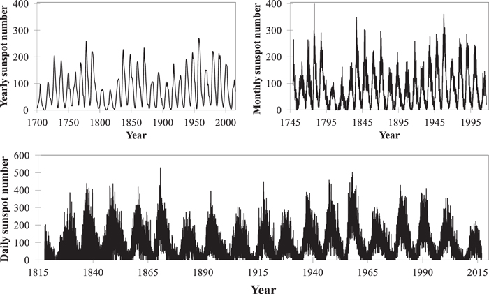
Figure 1. New sunspot number series for raw yearly (top left panel), monthly (top right panel), and daily (bottom panel) data.
Download figure:
Standard image High-resolution imageIn order to study and quantify the behavior of a process at unusually large or small levels, EVT is one of the statistical disciplines that have most commonly been used in the last few decades (Coles 2001). There are several ways to apply EVT to the study of extreme events. One that has been extensively used focuses on the generalized extreme value (GEV) distribution that models block maxima of the variables (Kharin & Zwiers 2000; Katz et al. 2002; García et al. 2007). However, if other information is available, the use of block maxima is a wasteful approach to extreme value analysis because many extreme events are rejected (Coles 2001), and a POT approach might be more appropriate. Both techniques are applied in this work because, despite the disadvantages of block maxima, it is important to study the maximum of each solar cycle.
First, the block maxima technique was applied to study the regional patterns of SN using different temporal scales. The maximum value of SN for each solar cycle (considered as a block) was selected leading to three different time series with 19, 25, and 29 values for daily, monthly, and yearly temporal scales, respectively. These three time series were fitted to a GEV Distribution. A complete description of GEV theory can be found in Coles (2001), for example. A brief description follows. GEV theory is a kind of "law of large numbers." It states that, for n large enough, the maximum of n independent identically distributed variables with a probability distribution function of type F tends to follow a GEV distribution with a probability distribution function given by
where μ, σ, and ξ are the location, scale, and shape parameters respectively, and [x]+ ≡ max(x, 0).
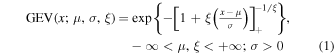
The POT technique considers all sample values that exceed a predefined upper threshold u. The probability distribution of the exceedances over the threshold can be modeled using the generalized Pareto distribution (GPD). In this technique, it is first necessary to select a threshold u whose choice could be difficult. A value of u that is too high leads to few exceedances and consequently high variance estimators. On the contrary, a value of u that is too low is likely to violate the asymptotic basis of the model, leading to bias (Coles 2001). Since the object of the study is the occurrence of high values of SN, the threshold applied, after a preliminary study to decide, was the 99.25th percentile for the daily SN time series. Two methods were used to check that this was indeed the best threshold to study extreme values in the sense of EVT. First, considering the mean residual life plot shown in Figure 2, there is some evidence for linearity above u = 329, which corresponds to the 99.25th percentile of the daily SN time series. Second, there is the stability of the parameter estimates fitting the GPD over a range of thresholds, considering that, for values above the chosen threshold, the shape parameter ξ does not change very much. As one observes in Figure 2, this method also confirmed that the 99.25th percentile of a daily SN time series was an optimal threshold.
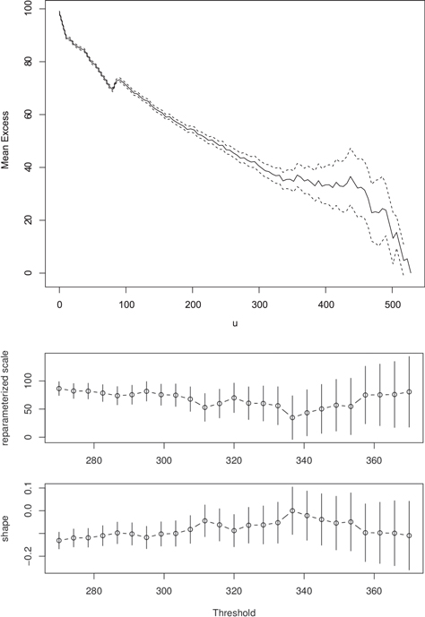
Figure 2. Mean residual life plot (top panel) and parameter estimates against threshold (two bottom panels) for daily SN.
Download figure:
Standard image High-resolution imageSince maximum values of SN are grouped into clusters one must expect that there may often be several consecutive days with maximum exceeding the threshold. These expected clusters of exceedances would therefore require a declustering procedure to be applied to identify within the sample approximately independent clusters of extreme observations to avoid short-range dependencies in the time series. The scheme used was "runs declustering" (Leadbetter et al. 1989). This consists of marking exceedances as belonging to the same cluster if they are separated by less than a fixed number of observations r called the run length. In this work, it is easy to justify the election of r = 13. This value is chosen because it is approximately half of the solar global rotation (Heristchi & Mouradian 2009). Then, for each cluster, the day with the maximum SN is chosen, and a set of C (number of clusters) extreme SN time series is calculated with the date and the intensity of the cluster.
These new time series were subjected to a GPD analysis. In the asymptotic limit for sufficiently large thresholds, with the observed daily sunspot number  , the distribution of independent excedances
  with
with  follows a GPD given by

with x > 0 and  , where σ is the scale parameter and ξ is the shape parameter
  (Coles 2001). Shape parameter values below zero indicate that the distribution has an upper bound, and values above or equal to zero indicate that the distribution has no upper limit (Coles 2001).
An important property in order to predict future extreme events is the RL. The N-year RL is the level expected to be exceeded once every N years, and was estimated for different values of N using both approaches. More details about RL estimations using block maxima and POT can be found in Coles (2001).
The parameters of the distribution for both the GEV and the GP distributions, Equations (1) and (2) respectively, were estimated by maximum likelihood using the in2extRemes statistical R software package for extreme values (Gilleland & Katz 2013). Once the parameters had been estimated, the confidence interval (CI) for each parameter was evaluated by a bootstrap procedure using 500 replicates (Gilleland & Katz 2013). The same procedure was used to estimate the RLs and their CIs with the bootstrap procedure.
The non-parametric Mann–Kendall test (Lettenmaier et al. 1994) was used as a practical approach to estimating trends in extremes. It was evaluated two-sidedly at two significance levels: 5% and 10%. If the test showed the trend to be statistically significant, the value of the trend was calculated by the distribution-free Kendall's tau-based estimator proposed by Sen (1968) and Lettenmaier et al. (1994). The trends in extreme time series obtained from the two techniques, cycle maxima and POT, were studied. Different scales were considered: daily, monthly, and yearly for cycle maxima, and only daily for the POT approach.
3. Results and Discussion
3.1. Block Maxima Approach
First, for the application of the block maxima approach, the maximum SN for each cycle was chosen for the different timescales used: yearly, monthly, and daily. These new time series were modeled by the corresponding GEV distribution. Figure 3 shows the diagnostic plots for assessing the accuracy of the GEV model fitted to the daily SN time series. The QQ-plot of empirical data quantiles against the GEV fit quantiles (top left panel) confirms the validity of the fitted model because the set of plotted points is near linear. The QQ-plot of randomly generated data from the fitted GEV against the empirical data quantiles with 95% confidence bands (top right panel) is a poorer fit to the model, though it is also near linear. These diagnostic plots for the daily SN time series represent the most unfavorable case, with the fits obtained from the plots corresponding to the monthly and yearly scales being better, maintaining near-linearity. Finally, the empirical density of the observed cycle maxima (solid black line, bottom panel) seems consistent with the fitted GEV density (dark blue dashed line). The diagnostic plots thus lend support to the fitted GEV model at the daily scale. As mentioned above, this statement also holds for the monthly and yearly scales.
Figure 3. Diagnostic plots from fitting the GEV to the cycle maximum sunspot number at a daily scale. Plots are a QQ-plot of empirical data quantiles against GEV fit quantiles (top panel), QQ-plot of randomly generated data from the fitted GEV against the empirical data quantiles with 95% confidence bands (middle panel), and (bottom panel) empirical density of the observed solar cycle maxima (solid black line) with GEV fit density (dark blue dashed line).
Download figure:
Standard image High-resolution imageTable 1 lists the results for the estimated GEV parameters with the corresponding 95% CI obtained by the bootstrap procedure for the three time series analyzed. The location parameter (μ) gives information about the mean values, the scale parameter (σ) about the variability, and ξ about the shape of the block maxima distribution. The shape parameter and its CI is nearly always negative, meaning the distribution has an upper bound. Only the 95% CI of the shape parameter for the monthly scale slightly surpasses zero.
Table 1. Estimates of the GEV Parameters and Their 95% Confidence Intervals Obtained by Bootstrapping
| Location (μ) [95% CI] | Scale (σ) [95% CI] | Shape (ξ) [95% CI] | |
|---|---|---|---|
| Daily | 366.29 [321.03, 411.25] | 85.83 [53.37, 124.13] | −0.49 [−1.10, −0.09] |
| Monthly | 215.19 [188.98, 246.10] | 68.02 [43.71, 89.31] | −0.24 [−0.65, 0.07] |
| Yearly | 149.50 [131.55, 175.17] | 53.48 [37.49, 69.77] | −0.34 [−0.78, −0.08] |
Download table as: ASCIITypeset image
As mentioned above, a well-known procedure for interpreting extreme values uses the RL. When using block maxima, the size of the block was taken as one solar cycle, different from one year. Then the N-cycle RL was estimated for N = 10, 50, and 100 solar cycles, corresponding approximately to RLs of 110, 550, and 1100 years, and the 95% CI was estimated using the bootstrap technique. Table 2 lists the estimates of the RLs for the three time series used (daily, monthly, and yearly) and for the three values of N chosen. For the daily time series, the results were surprising. It was expected that the 10-cycle RL would lie inside the block maxima SN range [202, 528] because the observed time series is longer than 110 years, but not the 50-cycle RL and even less so the 100-cycle RL because they correspond to values of N greater than the number of observed solar cycles at the daily scale (N = 19). These last two values (50-cycle RL = 501.05, 100-cycle RL = 507.68) were actually also inside the mentioned interval. The RL plots are shown in Figure 4 for the three timescales used. For the daily case, the extrapolation for the 50- and 100-cycle RLs given by the solid line indicates a value lower than the highest observed one, though SN = 528 is inside the 95% CI uncertainty of the RL for both the N = 50, and the N = 100 solar cycles. Therefore, an interesting result is that the RL is reaching a plateau, and it will be difficult to attain observed values in the future greater than SN = 528. These results must be considered with some caution, however, because RLs were estimated for a longer period than the observed one. The same behavior was found for the monthly and yearly time series.
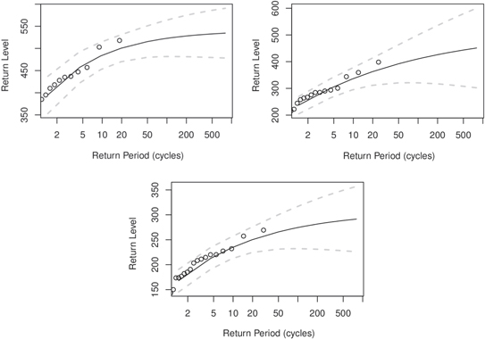
Figure 4. Return level plot (log scale) of cycle maxima using daily data (top left), monthly data (top right), and yearly data (bottom), with 95% normal approximation pointwise confidence intervals (dashed lines).
Download figure:
Standard image High-resolution imageTable 2. Different Estimates of the Return Level and Their 95% Confidence Intervals Obtained by Bootstrapping Using the Block Maxima Approach
| 10-cycle (110 year) RL | 50-cycle (550 year) RL | 100-cycle (1100 year) RL | |
|---|---|---|---|
| Daily | 474.91[441.48, 505.23] | 504.44[464.82, 545.77] | 513.03[462.53, 573.55] |
| Monthly | 328.78[294.39, 367.97] | 381.12[321.93, 456.59] | 396.51[320.44, 498.41] |
| Yearly | 230.81[207.45, 251.54] | 258.90[226.66, 292.59] | 267.11[231.32, 306.46] |
Download table as: ASCIITypeset image
3.2. Peaks-over-threshold Approach
The POT approach was also used to study the extreme SN for the daily time series. The definition of u = 329 as an appropriate threshold led to 505 exceedances over the whole period. In order to verify the condition of independent extreme observations, the aforementioned run declustering technique was applied with r = 13. This yielded 115 independent clusters with many solar cycles showing several extreme SN, and some of them showing none when the SN was lower than the chosen threshold. The range of these values was [330, 528]. This new time series with 115 observations was fitted with a GPD. Table 3 lists the estimates for the scale and shape parameters and the 95% CIs obtained by bootstrapping. The shape parameter is negative even considering the 95% CI, implying an upper bound of the extreme SN distribution, just as had been found with the GEV distribution. Figure 5 shows the diagnostic plots for the GP fit to the maximum SN from the daily time series. The plots confirm the validity of the fitted model. In particular, both QQ-plots are near linear.

Figure 5. Diagnostic plots from fitting a GPD to the maximum SN at a daily scale. Plots are a QQ-plot of empirical data quantiles against GP fit quantiles (top panel), QQ-plot of randomly generated data from the fitted GP against the empirical data quantiles with 95% confidence bands (middle panel), and (bottom panel) empirical density of the observed maxima SN (solid black line) with GP fit density (dark blue dashed line).
Download figure:
Standard image High-resolution imageTable 3. Estimates of the GPD Parameters and Their 95% Confidence Intervals Obtained by Bootstrapping
| Scale (σ) [95% CI] | Shape (ξ) [95% CI] | |
|---|---|---|
| Daily cluster maxima | 54.16[43.32, 71.55] | −0.18[−0.39, −0.04] |
Download table as: ASCIITypeset image
For this second technique, RLs were also estimated from the independent threshold exceedances of the sunspot number. The same values for N considered before were used, but considering the RL in years instead of cycles. The results are presented in Table 4. The values are greater than when using block maxima, with the 110 year RL (the 550- and 1100 year RLs) being lower (higher) than the observed maximum SN = 528. These results are confirmed by the RL plot in Figure 6, in which the solid black line shows the RL for each return period and the dashed gray lines show the 95% normal approximation pointwise CIs. One observes that the RL increases with the return period with a greater slope than that corresponding to the RL plot shown in Figure 4. That is why the 550- and 1100- RLs are greater than 528.
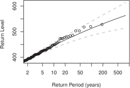
Figure 6. Return level plot (log scale) for maximum SN at the daily scale with 95% normal approximation pointwise confidence intervals.
Download figure:
Standard image High-resolution imageTable 4. Different Estimates of the Return Level and Their 95% Confidence Intervals Obtained by Bootstrapping Using the POT Approach
| 10-cycle (110 year) RL | 50-cycle (550 year) RL | 100-cycle (1100 year) RL | |
|---|---|---|---|
| Daily | 517.55[479.10, 556.00] | 542.60[488.12, 597.07] | 551.23[489.74, 612.58] |
Download table as: ASCIITypeset image
3.3. Trends in Extreme SN Time Series: Mann–Kendall Test and Sen Slope
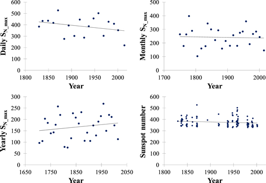
Finally, as mentioned in the Methods section, trends in the extreme time series obtained from the two techniques were studied using the Mann–Kendall test (Mann 1945; Kendall 1975) and the value of the slope of the trend evaluated by Sen's method (Sen 1968), both from data corresponding to the new version of the sunspot number index. To carry out this analysis, the time series obtained from the use of block maxima and POT approaches were used. For the first time, the maxima were selected for each solar cycle in the three different scales (daily, monthly, and yearly). For the second, all the independent exceedances of the threshold u = 329 after declustering the daily time series were chosen. Figure 7 shows the four extreme time series analyzed and the linear trends. Table 5 lists the results for the statistical significance of the trends according to the Mann–Kendall test and to the value of the slope obtained by Sen's method for the selected data.
Figure 7. Trends of the solar maxima per cycle at daily (top left panel), monthly (top right panel), and yearly (bottom left panel) scales, and of the independent exceedances above u = 329 (bottom-right panel) from the new sunspot number series. The solid lines represent the linear trends.
Download figure:
Standard image High-resolution image
Table 5. Results According to the Mann–Kendall Test and Sen Slope for the Maxima per Cycle for the Daily, Monthly, and Yearly Data, and for Daily Values Exceeding u = 329
| Mann–Kendall Test (τ) | Mann–Kendall Test (p-value) | Sen Slope | |
|---|---|---|---|
| Daily maxima per cycle | −0.758 | −0.224 | −42.857 |
| Monthly maxima per cycle | −0.023 | −0.491 | −1.208 |
| Yearly maxima per cycle | 1.107 | 0.134 | 13.811 |
| Daily SN exceeding u = 329 | −2.229 | −0.013 | −1.667 |
Download table as: ASCIITypeset image
The results show negative trends for three of the four extreme time series studied, with only the trend of the yearly maximum time series per cycle being positive. Note that daily and annual maximum series per cycle have high Sen slope values in absolute terms. The daily maxima per cycle time series show an important decreasing trend; though, it is not statistically significant, even at the 10% significance level, according to the Mann–Kendall test. For the daily time series that began in 1818, the first solar cycle, corresponding to Solar Cycle 6, was ending, and the maximum recorded (SN = 220) was not considered in this study due to its being underestimated. Since it is an important solar cycle because it belongs to the Dalton Minimum epoch, we studied what would happen if we included it. We found that the trend would also be negative (Sen slope = −6.67) if it were included.
The sign and the value of a trend are connected to the study period. The yearly SN time series spans from 1700 to 2015, and includes different subperiods with low solar activity: the end of the Maunder minimum, the Dalton minimum and the Gleissberg minimum. The first one, the Maunder minimum, appears only in the yearly SN time series, and introduces low SN values that lead to an increasing trend (Figure 7—bottom left panel). Moreover, the largest values for the SN maxima in the case of the yearly data are reached during the 20th century, while in the cases of the monthly and daily data they occur during the 18th and 19th centuries, respectively. Since the daily and monthly SN time series are shorter and have fewer subperiods of low solar activity, the trends become more negative. Also, for the yearly time series, the smoothing of the daily SN could introduce low values, which might contribute to a different sign of the trend. It can be seen that the trend for the SN values, which exceed the threshold u = 329 after declustering the daily data is also negative and with high a significance level. The value of the Sen slope obtained in this case (−1.667) is similar to that obtained for the monthly time series according to the block maxima approach (−1.208). Furthermore, we would emphasize that for the POT approach few daily SN values between Solar Cycles 12 and 15 exceed the threshold u = 329. Those solar cycles lie in a secular Gleissberg minimum.
4. Conclusions
This work has presented a survey of solar activity by applying EVT to the new version of the sunspot number index (Version 2) at daily (1818–2016), monthly (1749–2016), and yearly (1700–2015) scales. To this end, we employed, on the one hand, the block maxima technique using the GEV distribution that models the time series including the maximum values of the SN for each solar cycle at yearly, monthly, and daily scales. On the other hand, we used at the daily scale only, the POT approach that considers all SN values that exceed a predefined upper threshold u after declustering, which can be modeled using the GPD. Furthermore, trends in the extreme of the SN time series obtained from the two techniques were studied according to the Mann–Kendall test and Sen's method.
With the application of the block maxima approach, the diagnostic plots confirmed that the model fits appropriately at daily, monthly, and yearly scales. The shape parameters obtained by this method were nearly always negative, implying an upper bound of the distribution. Therefore, a maximum value for the SN has been reached for the study period, though this is compatible with the fact that, in the future, a new maximum higher than the observed could be recorded. The RLs obtained were (1) 474.91, 504.44, and 513.03 at the daily scale; (2) 328.78, 381.12, and 396.51 at the monthly scale; and (3) 230.81, 258.90, and 267.11 at the yearly scale, for N = 10, 50, and 100 solar cycles, corresponding approximately to 110, 550, and 1100 year RLs, respectively. Furthermore, due to the extent of the observed time series, it was expected that the 10-cycle RL would lie within the block maxima daily SN range of 202–528 because this interval is longer than 110 years, but not the 50-cycle RL and even less so the 100-cycle RL because these last two ranges are greater than the number of solar cycles observed at a daily scale. Therefore, according to these results, it seems that the RL is reaching a plateau and that it would be difficult to achieve observed daily SN values in the future greater than SN = 550. Of course, we note that these results must be considered with caution because RLs were estimated for a longer period than the observed one. The same behavior was found for the monthly and yearly scales.
In the POT approach, two methods were used to obtain the best threshold u with which to study extreme values of the solar activity at the daily scale: (1) considering the mean residual life plot, and (2) considering the parameter estimates for different thresholds with the daily SN. The threshold selected thus corresponded to the 99.25th percentile and u = 329 of the daily SN time series. To identify independent clusters of extreme observations, we selected a run length equal to r = 13 because this value is approximately half the solar global rotation. For each cluster, the day with the maximum SN was selected. With this technique, the shape parameter was negative even considering the 95% CI, i.e., the extreme SN distribution presents an upper bound, as was obtained with the block maxima approach. The RLs obtained in this case were 517.55, 542.60, and 551.23 for N = 110, 550, and 1100 years, respectively. Note that these values are higher than using the block maxima technique. Moreover, the 110 year RL (the 550- and 1100 year RLs) is lower (are higher) than the daily maximum observed value: SN = 528.
The Mann–Kendall test and the Sen slope gave negative trends for three of the four extreme time series studied (monthly and daily sunspot number maxima per cycle, and POT after declustering the daily sunspot number data). The yearly maxima time series per cycle was the only case of positive trend. Only the trend obtained with the POT approach for the daily data was statistically significant. The daily maxima time series per cycle also showed an important decreasing trend, though, as noted above, it was not statistically significant. In this particular case, Solar Cycle 6 was excluded because daily data for this solar cycle are only available for its last part, probably after the maximum had been reached. However, even if this underestimated point had been included in the analysis, the trend would still have been negative (Sen slope = −6.67). It is worthy of mention that, with the POT approach, few daily SN values corresponding to Solar Cycles 12–15 surpass the u = 329 threshold. Those data lie in a secular Gleissberg minimum.
Today, we know the history of solar activity during the Holocene (the last 11 millennia approximately) thanks to the cosmogenic radionuclides (e.g., Beer et al. 2012; Usoskin 2017). The most useful cosmogenic isotopes for solar activity reconstruction are radiocarbon 14C and beryllium 10Be. These reconstructions (see, for example, Usoskin et al. 2016a) have shown that over the millennia the Sun has gone through episodes of high, normal and low solar activity. Between episodes of high and low solar activity (usually named as Grand Maxima and Grand Minima, respectively), the Maunder Minimum and the Modern Grand Maximum are noteworthy. Therefore, a natural extension of this work would be the application of the EVT to these millennial time series.
It is worthy of mention that our results do not contain anything that can be related directly to a prediction about the future level of solar activity in the next decades and, even less, about the role of the Sun in the future climate of the Earth. Recent studies have shown that global warming could not be stopped even if a Grand Minimum of solar activity occurred in this century (Ineson et al. 2015; Maycock et al. 2015; Chiodo et al. 2016), as it happened in the 17th century (Eddy 1976; Usoskin et al. 2015).
Support from the Junta de Extremadura (Research Group Grant GR15137) and from the Ministerio de Economía y Competitividad of the Spanish Government (AYA2014-57556-P) is gratefully acknowledged.