


Abstract
We present a database of 3137 solar flare ribbon events corresponding to every flare of GOES class C1.0 and greater within 45° from the central meridian, from 2010 April until 2016 April, observed by the Solar Dynamics Observatory. For every event in the database, we compare the GOES peak X-ray flux with the corresponding active region and flare ribbon properties. We find that while the peak X-ray flux is not correlated with the active region unsigned magnetic flux, it is strongly correlated with the flare ribbon reconnection flux, flare ribbon area, and the fraction of active region flux that undergoes reconnection. We find the relationship between the peak X-ray flux and the flare ribbon reconnection flux to be  . This scaling law is consistent with earlier hydrodynamic simulations of impulsively heated flare loops. Using the flare reconnection flux as a proxy for the total released flare energy E, we find that the occurrence frequency of flare energies follows a power-law dependence:
  for
for  , consistent with earlier studies of solar and stellar flares. The database is available online and can be used for future quantitative studies of flares.
Export citation and abstract BibTeX RIS
1. Introduction
Solar flare emission over a wide range of electromagnetic wavelengths is a result of the rapid conversion of free magnetic energy stored in the sheared and/or twisted magnetic fields of active regions (ARs; Priest 1981; Forbes 2000; Fletcher et al. 2011; Hudson 2011; Shibata & Magara 2011; Kazachenko et al. 2012). Large flares are often accompanied by coronal mass ejections (CMEs; Andrews 2003), but not all flares are associated with CMEs (Hudson 2011; Sun et al. 2015), and some CMEs occur without any flare emission (Robbrecht et al. 2009; D'Huys et al. 2014). The total energy released during solar flares typically ranges between 1029 to 1032 erg (e.g., Emslie et al. 2012).
Flare ribbons are enhanced Hα and 1600 Å UV emission intensity structures in the transition region and the upper chromosphere at the height of approximately 2000 km. The enhanced emission is thought to occur in response to the precipitation of non-thermal particles accelerated either directly or indirectly by magnetic reconnection (Forbes 2000; Fletcher et al. 2011; Qiu et al. 2012; Longcope 2014; Li et al. 2014, 2017; Graham & Cauzzi 2015; Priest & Longcope 2017). Therefore, the flare ribbons correspond to the footpoints of newly reconnected flux tubes in the flare arcade.
The traditional CSHKP model of the two-ribbon eruptive flare (Carmichael 1964; Sturrock 1966; Hirayama 1974; Kopp & Pneuman 1976), shown in Figure 1(a), is able to explain many of the generic, large-scale observational properties of solar flares. Several three-dimensional (3D) generalizations of the CSHKP scenario have been proposed in the form of cartoons (Moore et al. 2001; Priest & Forbes 2002), quantitative topological models (Longcope et al. 2007), and analytic flux rope solutions (Isenberg & Forbes 2007). Figure 1(b) shows the Longcope et al. (2007) schematic of the CSHKP scenario where reconnection occurs at several sites to create the 3D coronal flare arcade loops and an erupting CME flux rope. Three-dimensional magnetohydrodynamics simulations of CME initiation all produce—to a greater or lesser extent—some version of the Figure 1(b) eruptive scenario (e.g., Török & Kliem 2005; Fan & Gibson 2007; Roussev et al. 2007; Lynch et al. 2009, 2016; Lugaz et al. 2011; Török et al. 2011; Aulanier et al. 2012).

Figure 1. Basic elements of the CSHKP two-ribbon flare model in (a) two dimensions (2D; from Forbes 2000) and (b) three dimensions (3D; from Longcope et al. 2007). Here, "R" indicates the location of the flare ribbons, "CS" the current sheet, "A" the overlying arcade, "P" the erupting plasmoid, "FR" the 3D flux rope, "PIL" the polarity inversion line, "X" the site(s) of magnetic reconnection, "S" the separatrix boundary of the erupting CME flux rope, and "C" the coronal flare loops formed by magnetic reconnection.
Download figure:
Standard image High-resolution imageFigure 1 shows that one of the main properties characterizing solar flares is the amount of magnetic flux that reconnects. While the reconnected flux cannot be measured directly from observations of the corona, the CSHKP model implies a quantitative relationship between the reconnection flux in the corona and the magnetic flux swept by the flare ribbon (e.g., Forbes & Priest 1984) given by

The left-hand side,  , denotes the coronal magnetic reconnection rate as the reconnection flux per unit time defined by the integration of the inflow coronal magnetic field, Bc, over the reconnection area, dSc. On the right-hand side, Bn is the normal component of the magnetic field in the ribbons that are the footpoints of the newly reconnected magnetic field lines in the corona. While direct measurements of Bc and dSc in the corona are not currently feasible, Bn and dSribbon are relatively straightforward to obtain from photospheric magnetogram and lower-atmosphere flare ribbon observations. Summing the total normal flux swept by the flare ribbon area,

yields an indirect, but well-defined, measure of the amount of magnetic flux processed by reconnection in the corona during the flare.
A number of studies have investigated the relationship between various flare properties and properties of the resulting CME, e.g., UV and HXR emission with the acceleration of filament eruptions (Jing et al. 2005; Qiu et al. 2010); CME acceleration and flare energy release (Zhang et al. 2001; Zhang & Dere 2006); and GOES flare class, flare reconnection flux, and the CME speed and flux content of the interplanetary CME (Qiu & Yurchyshyn 2005; Qiu et al. 2007; Miklenic et al. 2009; Hu et al. 2014; Salas-Matamoros & Klein 2015; Gopalswamy et al. 2017). However, in most of these analyses, the underlying data for the flare ribbon properties were of limited accuracy and involved different sets of instruments that required time-consuming co-alignment, making the systematic comparison of flare ribbon properties difficult for large numbers of events.
The launch of the Solar Dynamics Observatory (SDO; Pesnell et al. 2012), with the Helioseismic and Magnetic Imager (HMI; Scherrer et al. 2012; Hoeksema et al. 2014) and the Atmospheric Imaging Assembly (AIA; Lemen et al. 2012) instruments, represents the first time that both a vector magnetograph and ribbon-imaging capabilities are available on the same observing platform, making co-registration of the AIA and HMI full-disk data relatively easy. In this paper, we present a database of flare ribbons associated with 3137 events corresponding to all flares of GOES class C1 and larger, with heliographic longitudes less than 45°, from 2010 April through 2016 April. Our intentions are twofold. First, we provide the reference for the data set by describing the key processing procedures. Second, we present the statistical analyses of the flare reconnection fluxes and their relationship with other flare and AR properties.
This is the first in a series of two papers. Here, we focus on the cumulative reconnection properties, while in the second paper, we will analyze their temporal evolution.
This paper is organized as follows. In Section 2, we describe the SDO data and the analysis procedure for correcting pixel saturation, creating the flare ribbon masks, and calculating the ribbon reconnection fluxes and their uncertainties. In Section 3, we summarize the database of events, describe the AR and flare ribbon properties calculated for each of our events, compare these to the flare GOES peak X-ray fluxes, and present the distribution of the magnetic energy estimates associated with the reconnection fluxes. In Section 5, we discuss our results, and in Section 6, we summarize our conclusions.
2. Data and Methodology
In this section, using an X2.2 flare in NOAA AR 11158 as an example, we describe how we correct the AIA 1600 Å saturated pixels (Section 2.1), identify the flare ribbons, and find the reconnection fluxes (Section 2.2).
2.1. Filtering the Pixel Saturation in AIA 1600 Å Observations
The key technical challenge in defining the set of pixels corresponding to the flare ribbon location, dSribbon, in the AIA image sequences is the correction of the saturated pixels caused by CCD saturation and pixel bleeding, and of the diffraction patterns from the EUV-telescope entrance filter. Unfortunately, existing software packages for automatic de-saturation of AIA images such as DESAT (Schwartz et al. 2015) are not applicable to the 1600 Å channel (G. Torre 2017, private communication). Here we present our own empirical approach to correct the intensities of "bloomed" pixels.
To describe the details of our saturation-correction approach, we use the SDO AIA observations of the well-known "Valentine's Day" flare as a representative example. This flare occurred in NOAA AR 11158 on 2011 February 15, 01:44 UT (Schrijver et al. 2011). The SDO AIA observations of this event were saturated during the impulsive phase, from 01:49 UT to 02:10 UT in the UV 1600 Å continuum as well as in other AIA bands. We re-examine this event in UV 1600 Å observations with 24 s cadence and 0 61 pixel resolution with the objective of removing the saturated pixels and reconstructing the evolution of the UV ribbons from the earlier and later (unsaturated) phases of the flare. We process the UV 1600 Å images in IDL using the aia_prep.pro SolarSoft package and co-align the AIA image sequence in time with the first frame.
Our saturation-correction approach includes the following steps. We first select the pixels above saturation level,  counts s−1, and the pixels surrounding them within 2 and 10 pixels in the x- and y-directions. We then replace each saturated pixel intensity with the value linearly interpolated in time between the individual pixel's previous and subsequent unsaturated values that bracket the saturation duration. Figure 2, left column, shows a sequence of original AIA 1600 Å images on 2011 February 15: top panel, before the impulsive phase when AIA observations had no saturated pixels (01:47 UT); middle panel, at the peak of the impulsive phase with the largest number of saturated pixels (01:52 UT); and lower panel, during the gradual phase with no saturated pixels (02:11 UT). Figure 2, right column, shows the saturation-corrected images which differ from the original images only in the location of the saturation-corrected pixels. This empirical approach, while not suitable for photometric analysis of the corrected images, does allow one to identify flare ribbon locations (compare the original and corrected panels of the middle row). Thus, the saturation-corrected 1600 Å image sequence provides sufficient information to determine the reconnected flux using Equation (2).
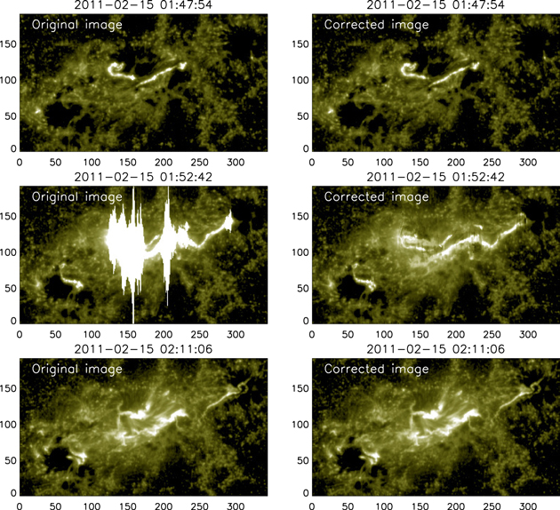
Figure 2. Snapshots of the 1600 Å flare ribbons in the X2.2 flare in NOAA AR 11158 observed by AIA on 2011 February 15. Left column: original AIA image sequence. Right column: saturation-corrected image sequence. Top row: no saturated pixels at the very beginning of the impulsive phase. Middle row: maximum number of saturated pixels. Bottom row: no saturated pixels during the gradual phase of the flare.
Download figure:
Standard image High-resolution imageFigure 3 shows the area-integrated light curves of the AIA 1600 Å image sequence at each step of the saturation removal procedure. The dashed−triple-dotted curve, labeled "Original saturated," plots the total number of counts in the saturated AIA 1600 Å image sequence. The period from 01:49 to 02:10 UT, shown with vertical dotted lines, indicates the duration of the pixel saturation in the sequence. The dashed curve, labeled "Saturated pixels set to zero," plots the total number of counts after the saturated pixels above the threshold level of Isat and the adjacent pixels have been removed. The dashed−dotted curve, labeled "Corrected image," plots the total counts after the saturated pixel values have been replaced by the interpolation in time between the unsaturated values of those pixels in the image sequence. Finally, the solid curve, labeled "Corrected image, ribbons," plots the light curve of the flare ribbons alone—the set of pixels that are identified by the ribbon search algorithm described in the next section. Note that the "Corrected image, Ribbons only" light curve is offset from the "Corrected image" curve by the total flux of the background that remains nearly constant during the flare. To summarize, Figure 3 quantitatively describes how much of the original image intensity is affected by the saturation and what fraction of this intensity is attributed to the flare ribbons using our saturation-correction approach.

Figure 3. Area-integrated light curves of AIA 1600 Å at different steps of the saturation removal procedure. The solid line shows the counts in the ribbons alone, i.e., the pixels above c = 8 times the background median value. The three vertical dotted lines correspond to three rows in Figure 2.
Download figure:
Standard image High-resolution image2.2. Constructing the Flare Ribbon Masks and Calculating the Reconnection Fluxes
To find the reconnection flux as defined by Equation (2), we need to know the flare ribbon location and the normal component of the magnetic field.
To identify the flare ribbon locations, we use the AIA 1600 Å saturation-corrected image sequence from Section 2.1 and the methodology of Qiu et al. (2002, 2004, 2007). We define an instantaneous flare ribbon pixel mask  in each pixel
  at each time step tk in the sequence with a value of 1 if the 1600 Å intensity is greater than an empirical ribbon-edge cutoff intensity, Ic, and with a value of zero if the intensity is below Ic. The cutoff intensity Ic for identifying the flare ribbon pixels ranges from the cutoff threshold c = 6 to c = 10 times the median image intensity at each time tk. This range is consistent with the range previously used for TRACE 1600 Å UV data (Kazachenko et al. 2012). Since the cutoff threshold for the "steady-state" UV brightening associated with plage regions is typically
  (see Figure 3 of Qiu et al. 2010), our empirical threshold range,
 ![$c\in [6,10]$](https://content.cld.iop.org/journals/0004-637X/845/1/49/revision1/apjaa7ed6ieqn9.gif) , is significantly greater than typical non-flare-related UV emission and is appropriate to capture the flare ribbons.
, is significantly greater than typical non-flare-related UV emission and is appropriate to capture the flare ribbons.
To find the normal component of the magnetic field, Bn, we use the full-disk HMI vector magnetogram data series (hmi.B_720s) in the form of field strength, inclination, and azimuth in the plane-of-sky coordinate (Hoeksema et al. 2014). We perform a coordinate transformation and decompose the magnetic field vectors into three components in spherical coordinates4
(Sun 2013). The derived radial component is the normal component Bn that we need in Equation (2). To avoid noisy magnetic fields, we only use magnetic fields greater than the flux density threshold  (see Figure 2 in Kazachenko et al. 2015).
The unsigned reconnection flux or unsigned magnetic flux swept up by the flare ribbons up to time tk is then calculated using the discrete observations as


where tHMI corresponds to the time of the measurement of the normal component of the magnetic field Bn, and the ribbon area  above the ribbon-edge cutoff intensity, Ic, is given by the discrete cumulative ribbon pixel mask
  multiplied by the pixel area dsij2. We correct each individual pixel area for foreshortening:
  , where
  is the angular distance between the central meridian and the pixel
  . The cumulative ribbon pixel mask
  is related to the instantaneous ribbon pixel mask
  in the following way:

Thus, the cumulative ribbon pixel mask represents the time integral (accumulation) of every flare ribbon pixel  that exceeds the 1600 Å intensity threshold at some instance from the first frame of the image sequence to tk. Figure 4 shows the cumulative ribbon pixel mask
  consisting of pixels above c = 8 times the background median value from the sequence of corrected images at the times shown in Figure 2.
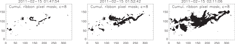
Figure 4. Evolution of the 1600 Å cumulative ribbon pixel mask  during the 2011 February 15 X2.2 flare.
Download figure:
Standard image High-resolution imageIn Figure 5, we summarize the temporal evolution of the flare ribbons associated with an X2.2 flare on 2011 February 15. The left panel shows the contours of the maximum flare ribbon area at the end of the AIA image sequence ( ) superimposed on the co-aligned HMI magnetogram before the flare at
  . The middle panel shows the temporal evolution of the ribbons, with the blue and red colors corresponding to the early and late stages of the flare respectively. Note that the
  color-coded bitmaps are plotted in reverse temporal order so that every individual pixel in the cumulative ribbon pixel mask is colored according to the time of its initial brightening.
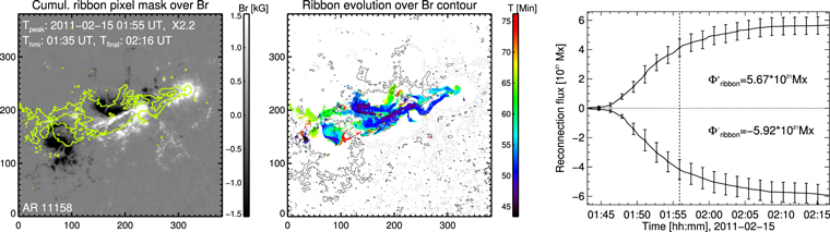
Figure 5. Left: HMI photospheric magnetogram Bn with the contours of the cumulative AIA 1600 Å flare ribbons at the flare end time overplotted. The times in the top-left corner are the GOES peak X-ray flux time (tpeak), time of HMI Bn observation (thmi), and the flare end time (tfinal). Middle: temporal and spatial evolution of the UV flare ribbons  with each pixel colored by the time of its initial brightening. Right: time profiles of the total reconnection flux in units of Mx integrated in the positive and negative polarities, respectively. The error bars in the reconnection flux indicate the range of uncertainty from the ribbon area identification. The vertical dotted line marks the GOES peak X-ray flux time.
  and
and  indicate positive and negative reconnection fluxes at the end of the sequence at time tfinal.
Download figure:
Standard image High-resolution imageThe right panel of Figure 5 shows the evolution of the magnetic fluxes swept up by ribbons in positive and negative polarities, the signed reconnection fluxes,  and
and  , respectively. To reflect the uncertainty in these estimates due to the ribbon area identification, we perform the entire pixel mask area calculation twice: once with the cutoff threshold c = 6, and again with c = 10. Then, the signed reconnection fluxes in each polarity at time tk are


where "+" and "−" refer to integration over the positive and negative polarities, respectively. In Figure 5, the reconnection fluxes in both polarities evolve nearly simultaneously. By tfinal = 02:16 UT, the positive and negative reconnection fluxes are  , and the total unsigned reconnection flux is
  . Theoretically, equal amounts of positive and negative flux should be reconnected. Hence, the balance between the two increases the credibility of the applied technique.
We estimate the errors in  and
and  at time tk using the uncertainty in the ribbon area (see error bars in Figure 5):
Typically, these range within 10% to 20% of  . Further in the text we do not take into account the uncertainty associated with the physical height of ribbon formation. The 1600 Å UV emission corresponds to the upper chromosphere and transition region whereas the photospheric magnetic field measurements are ∼2 Mm below this. The differences in normal field strength at the photosphere and at the ribbon formation height typically lead to a maximum decrease in the total reconnection flux of 10%–20% (Qiu et al. 2007; Kazachenko et al. 2012).
3. Database Description
3.1. Flare Ribbon Event List
The flare ribbon catalog RibbonDB contains properties of the ARs and flare ribbons for all well-observed flares of GOES class C1.0 and larger in the SDO era, from 2010 April until 2016 April. We used the existing Heliophysics Event Catalog (HEC) maintained by the INAF-Trieste Astronomical Observatory to select the events for our flare ribbon catalog. We chose flares within 45° from the central meridian to minimize projection effects. We also excluded events that were missing the AR number. We used get_nar.pro from SolarSoft to obtain the AR location coordinates for events with missing AR coordinates. These criteria resulted in 3137 flares for our RibbonDB catalog, including 17 X-class, 250 M-class, and 2870 C-class flares (see Table 1). Each entry contains the following information from the HEC: flare start time, flare peak time, flare end time, flare peak X-ray flux (flare class), flare heliographic longitude and latitude, and AR number. Figure 6 shows the monthly international sunspot number and the number of C-, M-, and X-class flares selected for the RibbonDB catalog as a function of time (upper panel) and also the time and location of ARs (lower panel). RibbonDB covers the first half of solar cycle 24, including its maximum around 2014 April. In the lower panel of Figure 6, the radius of each AR circle is proportional to the cumulative peak X-ray flux over the AR's lifetime. The ARs with the largest cumulative peak X-ray fluxes are NOAA AR 12192 (24 flares equivalent to 9 X1 flares in peak X-ray flux), NOAA AR 11429 (13 flares equivalent to 6 X1 flares), and NOAA AR 11515 (26 flares equivalent to 3 X1 flares).
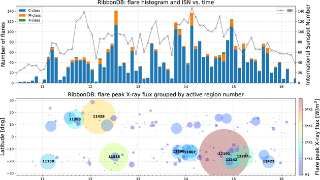
Figure 6. Top panel: number of C-, M-, and X-class flares each month in the flare ribbon database RibbonDB (left axis) and sunspot number from 2010 April until 2016 April (right axis). Bottom panel: flare peak X-ray flux and location on the disk grouped by AR vs. time; circle size and color correspond to the peak X-ray flux summed over each AR number.
Download figure:
Standard image High-resolution imageTable 1. Number of C, M, and X Flares and Their Corresponding Percentages in the RibbonDB Catalog
| Class | Number of Flares | Percentage, % |
|---|---|---|
| C | 2870 | 91.5 |
| M | 250 | 8.0 |
| X | 17 | 0.5 |
| T | 3137 | 100.0 |
Download table as: ASCIITypeset image
Figure 7 shows four representative events from our RibbonDB catalog, ranging from GOES C1.6 to X5.6 class, in the same format as Figure 5.

Figure 7. Representative flare ribbon events from the database in the same format as Figure 5. From top to bottom, the flare classes and GOES X-ray flux peak times are C1.6 on 2011 March 31 at 22:21 UT, C3.9 on 2012 June 17 at 17:39 UT, M6.7 on 2013 April 11 at 07:15 UT, and X5.6 on 2012 March 07 at 00:23 UT.
Download figure:
Standard image High-resolution image3.2. Active Region and Flare Ribbon Properties
For each event in the database, we use the AIA 1600 Å image sequence, of 24 s cadence and  spatial resolution, and a pre-flare HMI vector field magnetogram, of 12 minute cadence and
  spatial resolution, to derive the flare-ribbon-pixel masks and the normal component of the magnetic field, Bn, respectively (see Section 2.2 for details).5
We use these observations to compute the following large-scale, event- and area-integrated quantities:
spatial resolution, to derive the flare-ribbon-pixel masks and the normal component of the magnetic field, Bn, respectively (see Section 2.2 for details).5
We use these observations to compute the following large-scale, event- and area-integrated quantities:


where  and
and  are the unsigned AR magnetic flux and AR area,
  and
and  are the unsigned flare ribbon reconnection flux and flare ribbon area,
  and
and  are the mean AR and ribbon field strengths, and
  and RS are the percentages of the ribbon-to-AR magnetic fluxes and ribbon-to-AR areas, respectively. We calculate all the ribbon-related quantities at the flare end time. The integration
  means the summation over the AR region of interest, and
  and
and  are the summations over the ribbon cumulative pixel mask at the c = 6 and c = 10 ribbon cutoff thresholds at
  . The AR region of interest is defined as an 800 × 800 pixel (400 × 400 arcsecond) rectangle centered on the AR. The coordinates of the AR center are derived from the HEC mentioned in Section 3.1.
As discussed in Section 2.2, the uncertainties in the ribbon reconnection flux and the ribbon area were obtained by varying the threshold of the minimum ribbon brightness c from 6 to 10 times the median background intensity. The errors in the unsigned reconnection flux and ribbon area are then

Table 2 summarizes the event information included in the RibbonDB catalog that is available online.
Table 2. Variables in the RibbonDBa Catalog for Each of Our 3137 Flare Ribbon Events
| Variable | Quantity | Description |
|---|---|---|
| tstart | tstart | Flare start time [UT] |
| tpeak | tpeak | Flare peak time [UT] |
| tfinal | tfinal | Flare end time [UT] |
| ixpeak | IX,peak | Peak 1–8 Å X-ray flux [W m−2] |
| lat | lat | Flare location latitude [deg] |
| lon | lon | Flare location longitude [deg] |
| arnum | ARnumber | AR number |
| phi_ar | ΦAR | Total AR unsigned flux [Mx] |
| phi_rbn | Φribbon | Total unsigned rec. flux [Mx] |
| dphi_rbn | ΔΦribbon | Recon. flux uncertainty [Mx] |
| s_ar | SAR | AR area [cm2] |
| s_rbn | Sribbon | Ribbon area [cm2] |
| ds_rbn | ΔSribbon | Ribbon area uncertainty [cm2] |
| r_phi | RΦ | % recon. flux to AR flux |
| r_s | RS | % ribbon area to AR area |
a http://solarmuri.ssl.berkeley.edu/~kazachenko/RibbonDB/
Download table as: ASCIITypeset image
3.3. Statistical Analysis
To quantitatively describe the relationship between the different properties of flares and ARs, e.g.,  and
and  , we use the Spearman ranking correlation coefficient,
  . Unlike the Pearson correlation coefficient that measures the linear relationship between two variables—and therefore is not suitable for nonlinearly related variables—the Spearman rank correlation provides a measure of the monotonic relationship between two variables. To estimate the errors in the correlation coefficient due to sampling, we use a bootstrap method: for that we repeatedly calculate
  for N out of N randomly selected data pairs with replacement, and then estimate the mean and standard deviation as
  (Wall & Jenkins 2012, Chapter 6). From this point forward, we will refer to the mean Spearman correlation
  as simply the correlation coefficient
  and its standard deviation
  as the correlation's statistical uncertainty.
We describe the qualitative strength of the correlation using the following guide for the absolute value of rs: ![${r}_{s}\in [0.2,0.39]$](https://content.cld.iop.org/journals/0004-637X/845/1/49/revision1/apjaa7ed6ieqn55.gif) —weak,
—weak, ![${r}_{s}\in [0.4,0.59]$](https://content.cld.iop.org/journals/0004-637X/845/1/49/revision1/apjaa7ed6ieqn56.gif) —moderate,
—moderate, ![${r}_{s}\in [0.6,0.79]$](https://content.cld.iop.org/journals/0004-637X/845/1/49/revision1/apjaa7ed6ieqn57.gif) —strong, and
—strong, and ![${r}_{s}\in [0.8,1.0]$](https://content.cld.iop.org/journals/0004-637X/845/1/49/revision1/apjaa7ed6ieqn58.gif) —very strong. When the correlation coefficient is moderate or greater (
—very strong. When the correlation coefficient is moderate or greater ( ), we fit the relationship between
  and
and  with a power-law function,

We use the Levenberg–Marquardt nonlinear least-squares minimization method to find the scaling factor a and exponent b.
4. Results
4.1. Peak X-Ray Flux Versus Flare Ribbon and Active Region Properties
Table 3 summarizes the properties of the ARs and flare ribbons listed in Table 2, their range, and correlation coefficient with the GOES peak X-ray flux. The "Active Regions" column lists the AR unsigned magnetic flux, area, and the mean magnetic field:  , SAR, and
  . The "Flare Ribbons" column lists the reconnection flux, flare ribbon area, and the mean magnetic field swept by the ribbons:
  ,
,  , and
, and  . The bottom row shows the fractions of magnetic flux and area of the whole AR involved in the flare reconnection,
  and RS. We discuss each of these relationships further in the text and in Figures 8–11.
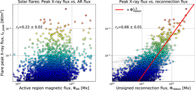
Figure 8. Scatter plots of peak X-ray flux vs. unsigned AR magnetic flux and flare reconnection flux. The Spearman correlation coefficients for these cases are listed in each panel. The power-law relationship  is shown in red.
Download figure:
Standard image High-resolution imageTable 3.
Active Region and Flare Ribbon Properties,  and
and 
| Active Regions | Flare Ribbons | |||||
|---|---|---|---|---|---|---|
| Quantity | Typical Range | Correlation | Typical Range | Correlation |

|
Figure |

|
![${{\mathbb{X}}}_{\mathrm{AR}}[{P}_{20},{P}_{80}]$](https://content.cld.iop.org/journals/0004-637X/845/1/49/revision1/apjaa7ed6ieqn76.gif)
|

|
![${{\mathbb{X}}}_{\mathrm{ribbon}}[{P}_{20},{P}_{80}]$](https://content.cld.iop.org/journals/0004-637X/845/1/49/revision1/apjaa7ed6ieqn78.gif)
|

|
∝ | |
| Φ | [28, 64] × 1021 Mx | 0.22 ± 0.01 | [5.4, 21] × 1021 Mx | 0.66 ± 0.01 |

|
Figure 8 |
| S | [78, 183] × 1018 cm2 | 0.14 ± 0.02 | [1.1, 3.7] × 1018 cm2 | 0.68 ± 0.01 |

|
Figure 9 |

|
[310, 442] G | 0.21 ± 0.02 | [408, 675] G | 0.24 ± 0.02 | ... | Figure 10 |
| RS | ... | ... | [0.9, 3.4]% | 0.53 ± 0.01 |

|
... |
| RΦ | ... | ... | [1.3, 5.1]% | 0.54 ± 0.01 |

|
Figure 11 |
Note. Quantity X is either the active region or flare ribbon magnetic flux Φ, area S, mean magnetic Field B, ribbon-to-AR fractions of the area RS, or magnetic flux RF. The typical range of each quantity is described as the 20th to 80th percentile ![${\mathbb{X}}[{P}_{20},{P}_{80}]$](https://content.cld.iop.org/journals/0004-637X/845/1/49/revision1/apjaa7ed6ieqn85.gif) . The relationship between
. The relationship between  and the peak X-ray flux is characterized by the correlation coefficient
  for variables with
  we find the coefficient b in the fit
  . For more details, see the figures.
Download table as: ASCIITypeset image
Figure 8 shows the scatter plots of the flare peak X-ray flux versus the total AR unsigned magnetic flux and the flare ribbon reconnection flux at  :
:  versus
  , left panel, and
  versus
  , right panel. While the flare peak X-ray flux has very little correlation with the AR magnetic flux,
  , it is strongly correlated with the flare ribbon reconnection flux,
  . The correlation is strong:
  . The power-law fit to
  versus
  yields
  .
.
If we restrict our analysis to stronger flares, M1 class and above, we find a weaker correlation coefficient with a larger standard deviation:  . This weakening is a result of the well-known problem in the statistics of range restriction (Pearson 1903), rather than a consequence of different physical processes governing smaller and larger flares. This effect reduces the correlation coefficients for flares in a smaller range of flare classes, e.g., flares larger than M1 or flares smaller than C5. For the same reason, we would expect a larger correlation between the flare peak X-ray flux and the reconnection flux if we include flare classes beyond the RibbondDB range.
In addition, we investigated the difference between using the normal component of the magnetic Bn field derived from the line of sight (LOS) versus the full vector magnetograms (as we do here). The normal component is then derived as  , where
  is the angular distance between the central meridian and the pixel
  . We find that the relationships between
  and
and  and
and  , their correlation coefficients, and the power-law exponents using BLOS are within the uncertainties of the estimates using the vector magnetic fields shown above.
Figure 9 shows the scatter plots of the flare peak X-ray flux versus total AR area ( versus SAR, left panel) and cumulative flare ribbon area at
  (
( versus Sribbon, right panel). Here, we find an even weaker correlation between the peak X-ray flux and the AR area (
 ) and a slightly stronger correlation between the peak X-ray flux and the cumulative flare ribbon area (
 ) than the AR flux and the ribbon reconnection flux, respectively.
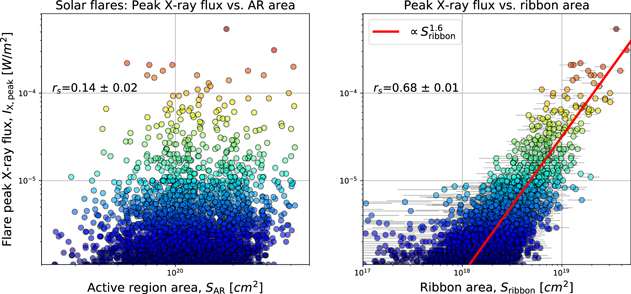
Figure 9. Scatter plots of peak X-ray flux vs. AR area and ribbon area. The Spearman correlation coefficients for these cases are listed in each panel. The power-law relationship is shown in red.
Download figure:
Standard image High-resolution imageWe further examine whether the mean magnitude of the normal magnetic field swept by the flare ribbons,  , is substantially different from the mean field of the whole AR,
  . Neither
  nor
nor  shows anything more than a weak correlation with the flare peak X-ray flux (0.21 ± 0.02 and 0.24 ± 0.02, respectively). This however does not contradict the known association between the strong gradients in the normal magnetic field across the AR polarity inversion line and the AR's flare and CME productivity (e.g., Welsch & Li 2008, and references therein). Figure 10 plots the distributions of
  and
and  for 3137 ribbon events. We find that the average of the
  field strength distribution is 100 to 200 G higher than the average of the
  distribution. The range between the 20th–80th percentiles for
  is 310–442 G (light blue shaded region), whereas the corresponding percentile range for
  is 408–675 G (light red shaded region). Figure 10 results confirm, in a statistical sense, that the magnetic fields that participate in the flare reconnection tend to be stronger fields than the AR as a whole.

Figure 10. Histograms for the mean magnetic field swept by ribbons (red) and of the whole AR (blue) for all events in the data set. Shaded areas show the ranges of magnetic fields where 20% to 80% of events reside.
Download figure:
Standard image High-resolution imageLastly, in Figure 11, we examine the relationship between the fraction of the AR magnetic flux that participates in the flare reconnection and the flare peak X-ray flux:  versus
  (see Equation (11)). The left panel of Figure 11 shows that the flare peak X-ray flux exhibits a moderate correlation with
  (
( ). The fit to the power-law relationship between the two quantities yields
  . The right panels of Figure 11 show the histogram distributions of
  in four ranges of flare classes: C1–M1 (dark blue), M1–M2.5 (light blue), M2.5-X1 (green), and X1-X5 (red). The distribution mean (vertical dashed line) and standard deviation are listed in each panel with the total number of events in the class range. For C1–M1 flares, the mean and standard deviation of
  is 3% ± 2%; for M1–M2.5 flares, 8% ± 4%; for M2.5-X1 flares, 12% ± 6%; and for X-class flares, 21% ± 10%. To summarize, both the mean and the width of the distributions of the reconnected flux fraction increase with the flare class strength.

Figure 11. Left panel: peak X-ray flux vs. reconnection flux fraction; four panels on the right: distribution of the number of flares of a certain class vs. the reconnection flux fraction. μ and σ are the mean and standard deviation of each distribution.
Download figure:
Standard image High-resolution image4.2. Occurrence Frequencies of Peak X-Ray Flux, Reconnection Flux, and Flare Magnetic Energy
To describe the statistical properties of solar and stellar flares, many authors have looked at the frequency distributions of various flare and CME parameters, such as flare duration, peak hard X-ray and soft X-ray fluxes, and total magnetic energy and its thermal, radiative, and the electron contributions (Drake et al. 2013; Maehara et al. 2015; Harra et al. 2016; Notsu et al. 2017). Since all of these quantities are products of the flare reconnection process (Forbes 2000), it is imperative to understand the quantitative distribution of flare reconnection fluxes and their associated magnetic energy release.
Following Aulanier et al. (2013), we estimate the energy released in the flare in terms of the properties of the reconnected magnetic field as
where f is the fraction of magnetic energy released as flare energy and V is the volume of reconnecting magnetic fields expressed in terms of the flare ribbon area  . We divide Sribbon by a factor of 2 to derive the signed from unsigned quantities. We also assume that all non-potential magnetic energy is released by the flare, i.e., f = 1. We note that Equation (15) differs from the flare energy estimates of Shibata et al. (2013) and Maehara et al. (2015) for stellar flares. Here, instead of the properties of the whole AR, we only use the flaring portion of the AR, as defined by the flare ribbons.
Figure 12 shows the occurrence frequencies for the GOES peak X-ray flux, ribbon unsigned reconnection flux, and the flare magnetic energy proxy:  ,
,  , and Eflare. The number of solar flares, proportional to their occurrence frequency, decreases dramatically as the flare energy increases. The fit to the power-law dependence of the peak X-ray flux distribution yields
  for
for ![${I}_{X,\mathrm{peak}}\,\in [{10}^{-6},5\,\times {10}^{-4}]\,{\rm{W}}\,{{\rm{m}}}^{-2}$](https://content.cld.iop.org/journals/0004-637X/845/1/49/revision1/apjaa7ed6ieqn134.gif) . The fit to the power-law dependence of the reconnection flux distribution yields
. The fit to the power-law dependence of the reconnection flux distribution yields  for
for ![${{\rm{\Phi }}}_{\mathrm{ribbon}}\in [8\times {10}^{20},{10}^{22}]\,\mathrm{Mx}$](https://content.cld.iop.org/journals/0004-637X/845/1/49/revision1/apjaa7ed6ieqn136.gif) . The fit to the power-law dependence of the distribution of flare energy, Eflare, yields
. The fit to the power-law dependence of the distribution of flare energy, Eflare, yields  for
for ![${E}_{\mathrm{flare}}\in [{10}^{31},{10}^{33}]\,\mathrm{erg}$](https://content.cld.iop.org/journals/0004-637X/845/1/49/revision1/apjaa7ed6ieqn138.gif) .
.
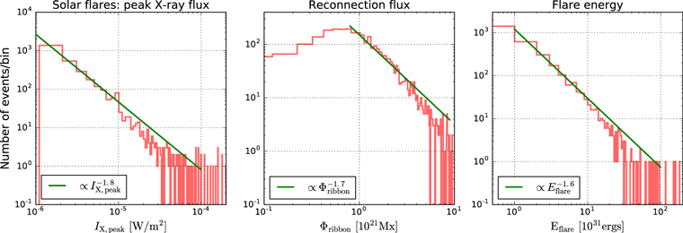
Figure 12. Histograms of the GOES peak X-ray flux, ribbon unsigned reconnection flux, and an estimate of the flare magnetic energy.
Download figure:
Standard image High-resolution imageWe also compare the distribution of our flare energy proxy derived from the reconnection flux with previous results for both solar and stellar flares. For solar flares, Crosby et al. (1993), Shimizu (1995), Aschwanden et al. (2000), and Qiu et al. (2004) have examined the occurrence frequency as a function of flare energy over  , which includes micro-flares and nano-flares. These distributions, obtained from EUV and soft and hard X-ray emission, are generally well-described by a simple power-law function,
  , with an index, α, of 1.5–1.9. For much larger stellar flares,
  erg, Maehara et al. (2015) and Notsu et al. (2017) found a power-law dependence,
  . In these estimates, the area of the starspot group was used as a proxy of stored magnetic energy, Eflare. Combining the solar and stellar flare results, Shibata et al. (2013) suggested that the frequency distribution should follow a universal power-law index,
  , for
, for  .
.
In this paper, we use high spatial resolution observations of flares on the Sun to estimate only the magnetic energy released during the flare, not the total AR magnetic energy. As shown in Figure 8, the total AR flux or area is only weakly correlated with the flare class. Hence, the total AR flux and area are, physically, not the best proxy for Eflare. The exponent for our distribution of flare energies is  , well within the range of exponents previously found for both stellar and solar flares (1.5–1.9).
5. Discussion
We have shown, in Figures 8–11, that while the GOES peak X-ray flux is only weakly correlated with the AR quantities ( , SAR), it is strongly correlated with the equivalent quantities derived from the flare ribbon observations (
 ,
,  ,
,  ).
).
Previous studies, e.g., Barnes & Leka (2008), have established that the more unsigned flux there is within an AR, the higher its overall rate of flare production, and the more likely the AR is to produce large (e.g., X-class) flares. Given the low correlation between the AR flux and the flare class that we find, how can the greater likelihood of large flares from large ARs be understood? If the magnetic reconnection processes responsible for the flare are universal (i.e., largely insensitive to active region size), then one may expect a universal distribution of flare frequencies as a function of energy (e.g., Wheatland et al. 2000; Wheatland 2010). In this way, a larger AR is more likely to produce flares of all classes and the likelihood of large flares will be enhanced relative to smaller ARs.
Understanding the stronger correlation between the reconnection flux and peak X-ray flux is fairly intuitive. The peak X-ray intensity is a measure of the ∼1–10 MK temperature emission response of the solar atmosphere to the rapid energy deposition supplied by magnetic fields that reconnected. It makes sense that the physical properties more closely associated with the flare reconnection process—our ribbon quantities—are more correlated with the resulting X-ray intensities than with the properties of the whole AR derived from the normal component of the AR magnetic fields.
Warren & Antiochos (2004) analyzed the hydrodynamic response of impulsively heated flare loops and found that the peak soft X-ray flux scales approximately with the flare energy as  , where V is the flare volume and L is the flare loop length. Writing V and L in terms of the flare ribbon area as
  and using the Equation (15) estimate for Eflare, we can rewrite the above relation as a function of our flare ribbon quantities:
Expressing the ribbon area in terms of the reconnection flux as  , we derive a theoretical scaling for the peak X-ray flux,

This estimate is remarkably consistent with our observed ( ,
,  ) relationship despite the approximations made above about the flare loop geometry. The power-law fit is
  (see Figure 8).
We also speculate that due to the Neupert effect (Neupert 1968; Veronig et al. 2002), the derived correlation between the reconnection flux and the peak soft X-ray flux will lead to a strong correlation between the peak reconnection flux rate and the peak hard X-ray flux, in agreement with earlier studies of individual events (e.g., Qiu et al. 2002; Veronig & Polanec 2015).
6. Conclusions
Since solar flares release energy stored in the magnetic field, the main property that describes the flare process is the amount of magnetic flux that reconnects, i.e., the reconnection flux. Previous estimates of the reconnection fluxes from observations of flare ribbon evolution were performed for only a limited number of events. The launch of SDO, with the HMI and AIA instruments on board, provided the first opportunity to compile a much larger sample of flare ribbon events. Taking advantage of this newly available data and our ribbon analysis techniques, we assembled a new RibbonDB catalog of 3137 events. The RibbonDB catalog contains flare ribbon and AR properties (Table 2) for every flare of GOES class C1.0 and greater within 45° of the central meridian, from 2010 April until 2016 April.
We analyze the properties of the ARs and flare ribbons in each event, including the AR magnetic flux, AR area, and the mean AR field strength, and the flare reconnection flux, flare ribbon area, and the mean strength of the fields swept by ribbons. We compare these quantities with the GOES peak X-ray flux as a proxy of radiative flare energy. Our findings are as follows.
- 1.We find strong statistical correlations between the flare peak X-ray flux and our derived flare ribbon quantities, cumulative ribbon area, and reconnection flux: Spearman correlation coefficient
 and , respectively. In contrast, the correlation between the peak X-ray flux and the corresponding AR quantities is weak: and .
 - 2.We find the power-law relationship between the peak X-ray flux and the ribbon reconnection flux to be. This exponent value is consistent with the Warren & Antiochos (2004) scaling law derived from hydrodynamic simulations of impulsively heated flare loops, thus indicating that the energy released during the flare as soft X-ray radiation originates from the free magnetic energy stored in the magnetic field released during reconnection.
- 3.We find a moderate correlation between the flare peak X-ray flux and the percentage of magnetic flux that gets reconnected:. Both the mean and the width of the distributions of the reconnected flux fraction increase with the flare class strength.
- 4.We find that the occurrence frequencies of the flare peak X-ray fluxes, reconnection fluxes, and the flare energies can be fit with the same power law,, with a power-law index . These results are consistent with previous studies of solar and stellar flares derived from AR properties.


![$\alpha \in [1.6,1.8]$](https://content.cld.iop.org/journals/0004-637X/845/1/49/revision1/apjaa7ed6ieqn163.gif)
This study is the first large-sample statistical analysis of the flare reconnection fluxes and their relationship with other flare and AR properties. While we focus on the cumulative reconnection properties here, in the second paper, we plan to extend our analysis to the statistical properties of the temporal evolution of flare ribbons, such as the ribbon speed and the reconnection flux rate. We believe that such a statistical approach is very beneficial since it enables us to investigate general trends that may be overlooked in case studies of individual events.
The RibbonDB catalog is available online6 in CSV and IDL SAV file formats, and can be used for a wide spectrum of quantitative studies in the future. For example, a comparison of reconnection fluxes with HXR emission, SEP fluxes, and CME and magnetic cloud properties would be valuable to clarify the relationship between the flares and ICMEs/CMEs, e.g., extending the Gopalswamy et al. (2017) analysis to a much larger number of events. Analysis of the outliers in the derived trends, for example, events with a large X-ray flux but small reconnection flux and vice versa, would be very interesting.
We thank Marc DeRosa and the AIA team for providing us with the SDO/AIA data. We thank the HMI team for providing us with the vector magnetic field SDO/HMI data. We thank George Fisher for reading and correcting the manuscript. We are grateful to Jiong Qiu and Dana W. Longcope for helpful discussions. We thank US taxpayers for providing the funding that made this research possible. We acknowledge support from NASA H-GI ODDE NNX15AN68G (M.D.K., B.T.W., B.J.L.), National Science Foundation, SHINE, AGS 1622495 (M.D.K., B.J.L.), NASA award NAS5-02139 (HMI, X.S.), Coronal Global Evolutionary Model (CGEM) award NSF AGS 1321474 (M.D.K., B.T.W., B.J.L.) and CGEM NASA award NNX13AK39G (X.S.).
Footnotes
- 4
Derivation of the radial component of the magnetic field is performed using the HMI pipeline code that is available to the public through the SDO Web page. Examples of usage can be found at http://jsoc.stanford.edu/data/hmi/ccmc/.
- 5
As the beginning and end times of the AIA 1600 Å image sequence, we chose one minute before the flare start time and the flare end time, respectively.
- 6