


Abstract
We investigate the physics of charged-particle acceleration at spherical shocks moving into a uniform plasma containing a turbulent magnetic field with a uniform mean. This has applications to particle acceleration at astrophysical shocks, most notably, to supernovae blast waves. We numerically integrate the equations of motion of a large number of test protons moving under the influence of electric and magnetic fields determined from a kinematically defined plasma flow associated with a radially propagating blast wave. Distribution functions are determined from the positions and velocities of the protons. The unshocked plasma contains a magnetic field with a uniform mean and an irregular component having a Kolmogorov-like power spectrum. The field inside the blast wave is determined from Maxwell's equations. The angle between the average magnetic field and unit normal to the shock varies with position along its surface. It is quasi-perpendicular to the unit normal near the sphere's equator, and quasi-parallel to it near the poles. We find that the highest intensities of particles, accelerated by the shock, are at the poles of the blast wave. The particles "collect" at the poles as they approximately adhere to magnetic field lines that move poleward from their initial encounter with the shock at the equator, as the shock expands. The field lines at the poles have been connected to the shock the longest. We also find that the highest-energy protons are initially accelerated near the equator or near the quasi-perpendicular portion of the shock, where the acceleration is more rapid.
Export citation and abstract BibTeX RIS
1. Introduction
Collisionless shocks exist in many astrophysical environments and are well-known sites of charged-particle acceleration. The underlying acceleration mechanism at shocks is reasonably well understood. Particles are accelerated as they pass through the strong plasma compression at the shock with a rate that depends partially on how well the particles are confined near the shock. In tenuous space plasmas, this is governed by the nature of the magnetic field. In diffusive shock acceleration theory (Axford et al. 1977; Krymsky 1977; Bell 1978; Blandford & Ostriker 1978), the evolution of the distribution function in space, time, and energy is determined by the cosmic-ray or Parker transport equation (Parker 1965). This equation includes the main charged-particle transport effects such as advection, energy change, drift, and spatial diffusion. The confinement of particles near the shock is related to diffusion coefficients, which depend on the magnetic field, including the power spectral density of its random component (Jokipii 1966). Drift motions also play an important role (Jokipii 1982) and also depend on the magnetic field. The rate of acceleration scales inversely with the diffusion coefficient (Forman & Drury 1983; Jokipii 1987, 1992), and because the diffusion of charged particles across the mean magnetic field is generally much smaller than that along the magnetic field (Giacalone & Jokipii 1999), shocks that move normal to the field are more rapid accelerators (Jokipii 1987). Thus, the magnetic field is critical for determining the maximum energy attainable from shock acceleration.
The efficiency of accelerating low-energy particles is also important for determining the overall intensity, and this also depends on the nature of the magnetic field. Diffusive shock acceleration (DSA) theory assumes a source of particles to be accelerated, but does not consider the origin of this source. The Parker equation is applicable if the pitch-angle distribution is nearly isotropic. In DSA theory, the intensity of particles falls off exponentially with distance from the shock. This intensity gradient causes a diffusive streaming of the particles. To be internally consistent, this anisotropy must be small, leading to a condition for the so-called "injection energy" for a quasi-planar shock (Giacalone & Jokipii 1999; Giacalone 2003; Zank et al. 2006). It can be written
where  is the shock ram energy, mp is the proton mass, U1 is the upstream plasma speed in the shock frame of reference, θ is the angle between the unit shock normal and the average magnetic field,
  , and
, and  .
.  and
and  are the diffusion coefficients perpendicular and parallel to the magnetic field, respectively, and
  is the antisymmetric diffusion coefficient.1
Under certain conditions, the injection energy given by Equation (1) has a very strong dependence on the shock-normal angle. For instance, for  and
and  , this gives
  . This expression has been used previously (e.g., Völk et al. 2003), and leads to the notion that nearly perpendicular shocks cannot accelerate low-energy particles. Some hybrid simulations, which satisfy these conditions, confirm this (Giacalone & Ellison 2000; Caprioli & Spitkovsky 2014). These conditions are not realistic for most astrophysical applications, however, because of the presence of preexisting turbulence. The conditions noted above unrealistically neglect particle motion normal to the average magnetic field. In the limit
  , Equation (1) reduces to
  , whereas in the limit
  , we obtain
  . These two expressions differ only by the value
  . This ratio depends on the magnetic field, including its turbulent component, and is not necessarily large. Magnetic field-line meandering, caused mostly by the largest scales in the fluctuating component of the magnetic field, leads to a significant enhancement in the motion of particles across the mean-magnetic field such that this term can be small. In this case, which is applicable to a wide range of astrophysical shocks, the acceleration of low-energy particles at perpendicular shocks can be nearly as efficient as that at a parallel shock. Hybrid simulations including preexisting broadband magnetic turbulence, through which the shock propagates, have revealed that even thermal plasma can be efficiently accelerated at a perpendicular shock (Giacalone 2005b).
As noted above, the threshold given by Equation (1) ensures internal consistency with DSA theory. Howerver, particles with energies lower than this may still be accelerated by shocks. The mechanism by which this happens is not well understood, nor is the number that is accelerated. The mechanism and number likely depend on the initial particle distribution, the shock parameters, and the nature of preexisting turbulence. The shock kinetic physics is important. As plasma is advected into the shock, incoming energy flux is converted mostly into enthalpy flux, which has a contribution from both the thermal and suprathermal components of the downstream particle distribution function. Hybrid simulations show that ∼20% of the energy flux incident on a strong parallel shock is converted into enthalpy flux of particles with energies greater than  (Giacalone et al. 1997).
Of course, shocks are not infinitely planar. On the one hand, for a curved shock, the angle between the mean-magnetic field and unit shock normal varies with position, and this leads to variations in the particle acceleration rate along the shock. This has important effects on the resulting particle intensity and energy spectra (Decker 1990; McComas & Schwadron 2006; Schwadron et al. 2008; Guo et al. 2010; Kòta 2010; Schwadron et al. 2015). On the other hand, magnetic field-line meandering creates variations in the angle between the local magnetic field and shock normal, leading to some places along the shock where the acceleration of low-energy particles is more efficient than others. This can lead to a "patchy" intensity of low-energy particles along the shock (cf. Giacalone 2005b; Giacalone & Jokipii 2009) with a characteristic scale likely on the same order as the magnetic turbulence coherence scale, Lc. When Lc is on the order of the radius of curvature of the shock, the physics of injection at a planar shock, as discussed above, is not necessarily applicable.
It is the purpose of this study to address the physics of particle acceleration at a spherical shock moving into a quasi-uniform plasma, which is applicable to a wide range of astrophysical phenomena. The most direct example is the acceleration of particles at a supernovae remnant (SNR), which is widely thought to be responsible for the production of galactic cosmic rays (GCR) with energies below the "knee" in the GCR spectrum at about 1015 eV. Because of computational limitations, we cannot feasibly model acceleration at a realistic SNR, but the results from our study provide important insights, discussed further in Section 4. In this study, we include a preexisting turbulent magnetic field embedded in the unshocked plasma and investigate its effect on the resulting energy spectra at various locations along the shock. The next section discusses the new numerical model, with more details provided in the Appendix. Section 3 presents the results of our numerical calculations, and Section 4 discusses some relevant astrophysical applications.
2. Numerical Model
We consider a spherically symmetric shock propagating with constant speed, Vsh, into a static and uniform plasma, which contains a turbulent spatially varying magnetic field. The magnetic field is decomposed into two components: one that is constant, and one that is random. The random component varies in space and time. In the unshocked plasma, its spatial dependence is determined from a sum of a very large number of individual plane waves with isotropically distributed wavevectors with random polarizations and phases. The amplitude of each individual wavemode is determined from a predefined Kolmogorov-like power spectrum. The result is a kinematically defined turbulent magnetic field with a uniform mean and a random component whose power-spectrum tensor is similar to isotropic Kolmogorov turbulence. We do not consider fluctuations caused by the streaming of energetic particles (e.g., Bell 1978; Lee 1983; Bell 2004) or by turbulent fluctuations in the plasma behind the shock (Giacalone & Jokipii 2007; Guo et al. 2012) in this study, and focus only on the effect of preexisting magnetic turbulence.
As the shock moves through the turbulent magnetic field, the shock modifies the field according to Maxwell's equations. Appendix A gives the details of our solution. In our model, the plasma flow speed is assumed to be radial and constant behind the shock, and the shock speed itself is also constant. Our model is not consistent with the standard Sedov blast-wave solution, in which the shock speed varies with time and the plasma speed behind the shock varies in space and time. The assumptions in our model are for convenience since they permit closed-form analytic solutions to the turbulent magnetic field behind the shock, provided it is known at some point far upstream in the unshocked plasma. Low-energy particles are likely not affected considerably by this assumption because the timescale for acceleration is shorter than the timescale associated with the evolution of the shock.
Figure 1 shows the magnetic field strength as a function of time (top panel), at a fixed spatial location, and as a function of radial distance from the center of the blast wave (bottom panel), at a fixed time, latitude, and longitude. We assume that the magnetic-field fluctuations are static in the plasma frame upstream of the shock; thus, since the ambient plasma is stationary, the field is constant when plotted as a function of time at a given location, as seen in the top panel prior to the shock crossing. Once the shock has passed the observer, the magnetic field is seen to vary with time because the observer is no longer in the fluid frame of reference.

Figure 1. Top: magnetic field strength as a function of time at a fixed location, as indicated. Bottom: magnetic field strength as a function of radial distance from the center of the blast wave at a fixed time, latitude, and longitude.
Download figure:
Standard image High-resolution imageShown in Figure 2 are projections of magnetic field lines on the x–z plane for three different values of the ratio of the turbulence variance to the mean-field squared, indicated with the symbol  , which increases from left to right. Two different times are shown, which separates the upper and lower panels of this figure. The magnetic field lines are determined by simultaneously solving the equations
  ,
,  , and
, and  , where s is the distance along a field line, B is the magnitude of the field, and
  is the magnetic field,
  , in Cartesian coordinates. The choice of field lines to display is arbitrary. We chose those that intersected or came close to the blast wave to give the best aesthetic visualization. The top three panels are for
  , which is when the blast-wave radius is larger than Lc, and
  for the bottom three panels, which is when the shock radius is smaller than Lc. Note that the angle between the unit normal to the shock and the magnetic field varies considerably along the shock front.
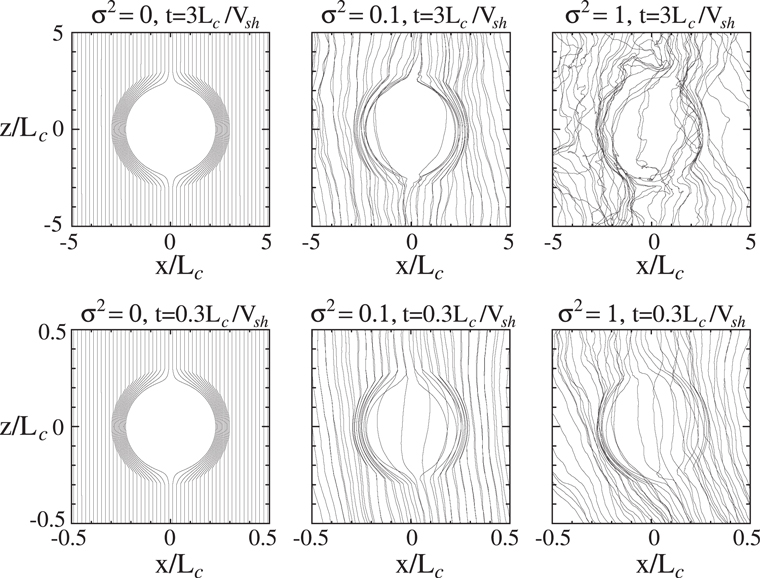
Figure 2. Magnetic lines of force projected onto the x–z plane, determined from the model magnetic field. The turbulence variance increases from the left to the right panels, and the time of the blast wave increased from the lower panels to the top panels, as indicated.
Download figure:
Standard image High-resolution imageUsing the electric and magnetic field solutions discussed in Appendix A, we numerically integrate the equations of motion of an ensemble of individual protons, given in cgs units as

where  is the momentum,
  is the velocity,
  is the electric field, e is the proton charge, and c is the speed of light.
  defines a standard spherical coordinate system, with θ being the polar angle. We use a numerical scheme known as the Burlisch-Stoer method (Press et al. 1986), which uses an adjustable time step in order to conserve total energy. Energy is conserved in our calculation to better than
  .
.
 and
and  are functions of all three spatial coordinates. Therefore our model allows for the motion of particles away from magnetic lines of force, which is artificially suppressed in models that use at least one ignorable spatial coordinate (Jokipii et al. 1993; Giacalone 1994; Jones et al. 1998). Thus, our model correctly treats cross-field transport including effects from field-line meandering as well as the local transport off of field lines.
We are interested in obtaining the distribution function of an ensemble of particles at a particular time, tmax. This is determined from the final positions and plasma-frame velocities of the protons. An individual proton is released at a time  , where ξ is a uniformly distributed random number between 0 and 1. The cube root follows by assuming a constant flux of source particles across the shock,
  , and noting that the surface area of the shock increases as it moves outward.2
n0 is the density of test particles upstream of the shock. We start the numerical integration of Equation (4) at t0, with an initial radial position taken to be at the same location as the shock at this time,
, and noting that the surface area of the shock increases as it moves outward.2
n0 is the density of test particles upstream of the shock. We start the numerical integration of Equation (4) at t0, with an initial radial position taken to be at the same location as the shock at this time,  , with an initial speed
  , as measured in the local plasma frame. The particle is released with a uniform probability of being placed anywhere on the shock surface, so the source only depends on radial position and time. The particles are also released isotropically in velocity space. The integration ends when time has advanced to tmax. The distribution function is then determined from the final velocities and positions of all the particles.
Table 1 lists the parameters of each of the numerical integrations performed in this study. There are three important length scales: (1) the gyroradius, rg0, of a charged particle moving with the initial speed at its release point,  in a field with a strength equal to that of the average field, B0 (
 , where
  is the cyclotron frequency); (2) the coherence scale of the magnetic fluctuations, Lc; and (3) the radius of the shock at the maximum time of the simulation,
  . Computational limits restrict us to study values of
  or lower. This is because the maximum time of the calculation is of this same order times the cyclotron period,
  , and we require a time step shorter than
  for numerical accuracy. We also integrate the trajectories of many millions of particles. We are not currently capable of simulating a realistic SNR blast wave, which for typical parameters has a radius some
  times larger than the gyroradius of protons. This is discussed further in Section 4, along with other relevant astrophysical examples.
Table 1. Summary of Simulation Parameters
| Run |

|

|

|
Realizations | plotted in |
|---|---|---|---|---|---|
| 1 | 104 | 5 | 1 | Ensemble | Figure 3 |
| 2 | 105 | 5 | 1 | Ensemble | Figures 3, 4, 5, and 7 |
| 3 | 105 | 5 | 1 | Single | Figures 5 and 9 |
| 4 | 106 | 5 | 1 | Ensemble | Figure 3 |
| 5 | 105 | 5 | 0.3 | Ensemble | Figure 8 |
| 6 | 104 | 50 | 1 | Single | Figure 9 |
| 7 | 106 | 0.5 | 1 | Single | Figure 9 |
Note. In all simulations: km s−1, the density compression ratio across the shock is 4 (strong shock limit) and the maximum shock radius is 5Lc.
  is the variance divided by the square of the mean field.
Download table as: ASCIITypeset image
In some of our simulations, each particle is followed in a different realization of the magnetic field, which is intended to give an "ensemble" average. We also consider the more realistic case in which the magnetic field realization is the same for every particle, however.
We have also performed two additional simulations of a planar-shock front in order to compare with the results from the spherical-shock case. We used the same model as that described in Giacalone & Jokipii (2009) for the planar-shock simulations. We chose parameters for the shock and magnetic turbulence to be identical to that used in Run 3 in Table 1, as well as the same maximum simulation time. For the planar-shock case, there is no adiabatic cooling of the particles. In one of the planar-shock simulations, the mean field is perpendicular to the shock-normal direction, and for the other simulation, the mean field is parallel to it.
3. Results
Figure 3 shows the final energy spectra, averaged over all particles at all locations, for three of our simulations. These correspond to runs 1, 2, and 4 in Table 1. Energy is measured in the local plasma frame of reference. The magnetic turbulence coherence scale, Lc, is varied from  (black histogram) to
  (red) to
  (blue). In each case, the ratio of the final shock radius to Lc is held fixed, and since Lc varies, so does the final shock radius. Thus, the blue spectrum, for example, corresponds to the largest final shock radius and the longest maximum time, tmax. This spectrum extends to the highest energy in this case because the particles have had the longest time to be accelerated.

Figure 3. Differential flux spectra as a function of kinetic energy for three different values of  : 104 (black), 105 (red), and 106 (blue). These are obtained from simulations 1, 3, and 4, in reference to Table 1, respectively. Kinetic energy is normalized to the shock ram energy,
  , and the differential flux is normalized to
  .
.
Download figure:
Standard image High-resolution imageThe peak in the spectrum for all three cases is at the injection energy, which is the same as the shock energy,  . For
. For  , the spectra fall off with decreasing energy due to adiabatic cooling of the particles in the downstream fluid flow. Above ER, there is a bump-like feature, extending to about
  , which is caused by particles that execute a single gyro-orbit around the shock front before being advected downstream. Because they drift along the shock during this single orbit in the same direction as the motional electric field, they gain a small amount of energy. This is a non-diffusive kinetic effect typically seen in test-particle simulations of low-energy particles moving in synthesized magnetic turbulence (cf. Giacalone 2005a; Giacalone & Jokipii 2009). This feature is not typically seen, however, in self-consistent hybrid simulations (e.g., Giacalone 2005b; Giacalone & Decker 2010) that include shock microstructure, such as the cross-shock potential, which is not included in our simplified model. Above this energy, the spectrum is approximately a power law up to about ∼50–100ER. The slope is somewhat smaller than that predicted by simple diffusive shock acceleration theory applied to a planar shock. This is mostly because the simulated spectrum includes contributions from particles upstream of the shock, whereas the theory only applies downstream. At higher energies, the spectra are steeper. This steepening is caused by the finite acceleration time, but because the "local" acceleration rate varies along the shock, this also effects the resulting shape of the spectrum at high energies. The rate is fastest where the local shock-normal angle is 90° (locally perpendicular) and slowest where it is 0° (locally parallel), as discussed by Jokipii (1982, 1987)), and also shown below in Figure 6(c). Consider the special case in which the acceleration rate is constant along the shock. In this case, we would expect the downstream spectrum to be a power law at low energies, and then become exponential at a characteristic energy that depends on the acceleration rate (see also Appendix B). If the shock is parallel, this energy is much lower than if the shock is perpendicular. In the spherical-shock case, the final spectrum differs from these two extremes because the acceleration rate varies.
Figure 4 shows a comparison of results between planar and spherical shocks. The black spectrum is the case of a spherical shock, Run 3 from Table 1, as discussed above. The red spectrum is that obtained from a simulation in which the shock front was taken to be planar and the average magnetic field is parallel to the shock normal, and the blue spectrum is for a planar perpendicular shock on average. In all cases, the spectrum is computed from the final plasma-frame velocities and averaged over all positions, both upstream and downstream of the shock. There is no adiabatic cooling in the planar-shock case, and therefore there are no particles below the injection energy. The blue spectrum extends to the highest energy, as expected, since the acceleration rate is the most rapid at a perpendicular shock. Since the maximum time is the same for all cases, a higher acceleration rate leads to a higher maximum energy. The energy spectrum for the spherical-shock case, shown in black, does not extend to as high an energy as that of the perpendicular shock and only slightly exceeds that of the planar parallel shock. It is clear that adiabatic cooling is also important in determining the final spectrum in the spherical-shock case.

Figure 4. Differential flux spectra as a function of kinetic energy for a spherical shock (black) and planar shocks (red and blue), as indicated.
Download figure:
Standard image High-resolution imageThe spectra shown in Figure 3 (and the black histogram of Figure 4) were averaged over the entire space, but as shown in Figure 5, the particle intensity is not uniform along the spherical shock. The figure shows a color-coded representation of the normalized flux, I, of high-energy particles with energies above 1000ER in the (x, z) plane, averaged over all y. I is defined

where dJ/dE is the differential intensity, determined from the distribution function by binning the particle final positions and velocities. The position is normalized to Lc. n0 is the number density of the "seed" particles. This is not the number density of the ambient gas, but it is reasonable to expect that they may be related. It is known that high-Mach shocks dissipate their energy by reflecting a fraction of the particles incident on the shock, creating suprathermal "specularly reflected" ions (Leroy et al. 1981; Sckopke et al. 1983; Winske 1985). It is reasonable to expect these to be further accelerated by the shock (e.g., Giacalone 2005b). Thus, n0 might reasonably be a fraction of the number density of the ambient gas that is specularly reflected by the shock.

Figure 5. Color-coded representations of the flux of particles with energies above 1000ER, normalized to  , at
, at  . I is given by Equation (3). The left panel shows the case in which each particle experienced a different magnetic field realization, thereby representing an "ensemble average"; whereas the right panel shows the results for the case in which only one magnetic realization was used. These results were obtained from simulations 2 (left) and 3 (right), respectively, in reference to Table 1. For this case, the ratio of the coherence scale to initial gyroradius of the particles is
  .
.
Download figure:
Standard image High-resolution imageThe left panel of Figure 5 is for the case in which a different realization of the turbulent magnetic field was used for each particle. It represents the ensemble average. The right panel shows the case in which each particle moved within the same magnetic field, defined by a single magnetic field realization.
The peak intensity is at the shock, which is at 5Lc, but I also varies along the shock surface. In the left panel of Figure 5, we note that the flux of accelerated particles is highest in the polar regions of the blast wave. This is where the magnetic field, on average, is close to the direction of the unit normal to the shock—the quasi-parallel portion. I also extends over a larger distance upstream—toward the uniform plasma outside the blast wave—in the polar regions. This is caused by the diffusive decay of particles into the upstream region. The associated diffusion coefficient in the direction parallel to the local field,  , is larger than that across it
  (e.g., Giacalone & Jokipii 1999). This results in a larger diffusive decay scale in the polar regions compared to the equator.
I is maximum in the polar region of the shock because the field lines in this region have been connected to the shock the longest, and the particles tend to remain close to magnetic lines of force. Thus, the particles collect at the poles. To show this, consider the geometry in Figure 6(a). At time T, a particular magnetic field line, in blue, makes an angle θ with respect to the unit normal to the shock, as indicated. This same field line was first crossed by the shock at the earlier time  , indicated in red. Thus, this field line is connected to the shock for a time
  . Note that the intersection point starts at the equator and moves poleward with time. Figure 6(b) shows the connection time normalized to the total time,
  , as a function of the angle θ. When
  , near the poles of the shock, this ratio is approximately one, which means that such a field line has nearly always been connected to the shock. Conversely, when
  ,
,  , meaning that the field line has only been connected to the shock for a very short time.

Figure 6. (a) Illustration of the shock at two different times, t = T (black circle), and  (red circle), and a single magnetic field line at the two different times, in blue. The field line is dashed for
  , the smaller shock radius. At t = T, the field line makes an angle θ with respect to the shock-normal direction, as indicated. (b) The ratio of the time over which the field line makes a connection with the shock,
  , to the total time, T, as a function of θ. (c) The acceleration rate of particles from diffusive shock acceleration theory for two different values of
  , as indicated, normalized to the rate at a parallel shock (
 ), as a function of θ. See text for more details.
Download figure:
Standard image High-resolution imageFor the case of a single realization, shown in the right panel of Figure 5, the intensity is more randomly distributed than in the case of the ensemble average. The intense regions are presumably related to the time over which the field lines have been connected to the shock, leading to "collection regions," but we did not attempt to establish this quantitatively.
The higher intensity of particles near the poles seen in the left panel of Figure 5 does not imply that this is where the acceleration is most rapid. The acceleration rate, in fact, is slowest at the parallel shock and fastest at the perpendicular shock (Jokipii 1982, 1987), as shown in Figure 6(c). This panel plots the acceleration rate, normalized to the rate at a parallel shock, as a function of θ for two different values of  , based on the expression derived in Appendix B. The high-energy particles, having the highest intensities at the poles, were initially accelerated closer to the equator, where the acceleration is more rapid, as discussed below.
Figures 7 and 8 show energy spectra computed from the final plasma-frame energy of the particles in two different regions of the sphere, separating those computed from the final locations of the particles from those computed using the initial locations. The top panels in both figures are the energy spectra of particles whose final polar angle,  is (a) near the equator (
 , where
  ), as indicated, in blue; and (b) near the upper polar region (
 ), in red. In the lower panel, the energy spectra are computed from the final energy of the particles, but are sorted by the initial polar angle where they were released,
  . For example, the blue spectra in the lower panels of Figures 7 and 8 show the final energy distribution of particles initially released near the equator (
 , where
  ); whereas the red spectra are for particles that were initially released near the upper pole (
 ).
).
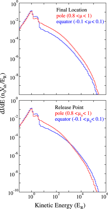
Figure 7. Differential intensity spectra, in units of  , as functions of energy normalized to ER for simulation 2 in Table 1. In all cases shown, the spectra were computed from the final energy of the particles, at
  . The top panel shows spectra computed in two separate polar angle bands, one near the equator (in blue, with the cosine of the polar angle indicated in the legend), and the other at the upper polar region of the sphere (in red). For the bottom panel, the energy spectra are computed from the final energy, but the two different polar-angle bands are determined from the initial locations, or release point, of the particles. μ and
  are defined in the text.
Download figure:
Standard image High-resolution image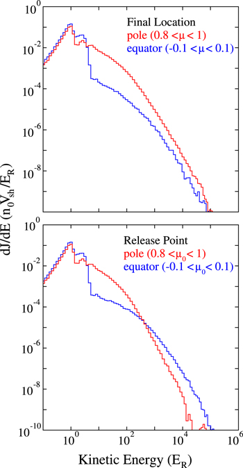

Download figure:
Standard image High-resolution imageAlthough the highest intensity of particles at the end of the simulation is reached at the poles, it is clear from the bottom panels of Figures 7 and 8 that the highest-energy particles initially encountered the shock near the equator. This is where the shock moves normal to the average magnetic field. Thus, particles are initially accelerated very rapidly near the equator, at the perpendicular shock. Because of the compression of the magnetic field at the shock, they drift along its surface, in the same direction as the motional electric field (in the shock frame of reference), and gain energy. They also remain near the field lines on which they began their motion. As the shock expands outward, the point of intersection of any given field line to the shock moves poleward, on average, as noted above. Thus, as the particles gain energy each time they cross the shock, they also collect at the poles. The rate of acceleration decreases with time because the local shock-normal angle becomes more parallel, on average, with time, as indicated in Figure 6.
Note also that the intensity of low-energy particles (below a few hundred ER) released at the equator is lower than those released at the poles. This indicates that the acceleration efficiency, or number of accelerated particles, is somewhat lower for particles injected near the equator than at the poles. However, the acceleration efficiency at the equator is sufficient, given the very high rate of acceleration there, that ultimately, the highest-energy particles in the system were initially released near the equator.
Figure 8 is of the same format as Figure 7, but differs in the variance of the upstream turbulence. Figure 7, which shows results from Run 5 in Table 1, is the case of a smaller variance of  ; in contrast, Figure 7 is for the case of
  (Run 2). We see the same overall behavior discussed above, but there are several noteworthy differences. For the case of a smaller turbulence variance, the vast majority of lower-energy particles, with energies between
  , were injected near the polar regions. Very few originated near the equator. This difference is considerably larger for the case of a smaller variance than for the larger variance used for Figure 7. The reason for this is that when the upstream turbulence has a small variance, fewer particles are injected at the quasi-perpendicular shock (cf. Giacalone 2005a). However, because the variance is smaller, the cross-field diffusion coefficient is also smaller (e.g., Giacalone & Jokipii 1999), and hence, the acceleration rate, which scales as the inverse of the diffusion coefficient, at the perpendicular shock is much higher than in the case of a larger turbulence variance (see the dashed curve in Figure 6(c)). Thus, although the rate of injection of particles released near the equator is lower, the acceleration rate is higher. Moreover, the weaker turbulence also leads to a larger parallel diffusion coefficient (weaker pitch-angle scattering, larger mean free path of scattering), leading to a much slower rate of acceleration at the parallel shock near the poles. Thus, the highest-energy particles, which ultimately collect near the poles, were initially released near the equator, despite the weaker turbulence. Note that for
  , the vast majority of the particles were released near the equator.
In the two previous figures, we focused on the differences between the injection and acceleration rates between the equator and poles of the shock in terms of the behavior of the ensemble average. These were cases in which each particle experienced a unique magnetic-field realization. For the case of a single magnetic-field realization, the results will differ from the ensemble average case, depending on the relative size of the shock and turbulence coherence scale. This is addressed in Figure 9. This figure shows results from three simulations, each of which considers a single magnetic field realization. The maximum shock radius is the same in all three cases, but the turbulence coherence scale, Lc, varies. The results are from from Runs 3, 6, and 7 in Table 1. The left panel is for the case of the highest value of Lc and lowest for that shown in the right panel. The turbulence variance is held fixed for these three cases at  . For the case in which
  , the field varies considerably over the shock front, but this variation is less when
  . As above, we show energy spectra as a function of the final plasma-frame energy of the particles. Colors are used to delineate different release locations, as defined by the initial "local" shock-normal angle,
  , at the time each particle was released. This is represented by
  . For instance, the blue spectra correspond to particles initially released where the local shock-normal angle was very nearly perpendicular to the shock normal, and the red spectra are for a locally parallel shock-normal angle.

Figure 9. Energy spectra based on the final velocities of the particles, but sorted by their initial release location relative to the "local" magnetic field.  , where
  is the angle between the local magnetic field and unit shock normal (radially outward) at the time each particle was released at the shock. In all cases, the maximum time, which is when the spectra are computed, are the same. Thus, the final shock radius is the same in all panels. The coherence scale of the fluctuations is varied. It is the largest in the leftmost panel and smallest in the rightmost panel.
Download figure:
Standard image High-resolution imageThe left panel of Figure 9 shows that particles that are initially injected where the local magnetic field is close to parallel to the shock normal are more efficiently injected than those where the local field is close to normal to the shock. For this case, the coherence scale of the turbulent fluctuations is smaller than the final shock radius, and obviously is smaller than the shock radius throughout the entire simulation. The results suggest that for this case, injection is very much a local process—that is, the injection is determined by the local shock-normal angle. This is consistent with previous studies of quasi-planar shocks that either do not include preexisting upstream magnetic turbulence (Burgess 1987; Giacalone & Ellison 2000; Caprioli & Spitkovsky 2014) or do not include magnetic field-line meandering (Baring et al. 1994). In contrast, for the case in which Lc is much smaller than the final shock radius, the difference between particles injected where the field is nearly parallel to the shock is much smaller than for particles injected where the field is more perpendicular. For this case, the acceleration efficiency at the perpendicular shock (on average) is quite high, even close to that at the parallel shock. This is consistent with the findings of Giacalone (2005a, 2005b). It should be noted that particles exist on average in the system many thousands, even millions, of gyroperiods from the time they are released to the maximum simulation time. Those that encounter the shock many times, they experience a wide range of local shock-normal angles each time they cross. The shock-normal angle when it is released is not the same the next time a particle encounters the shock.
4. Implications for Astrophysical Shocks
Supernovae (SNe) blast waves are examples of an approximately spherically propagating shock front moving into a quasi-uniform medium containing a large-scale turbulent magnetic field. Older SN shocks have typical radii of several parsecs. Assuming  pc, a shock speed of
  km s−1, and an interstellar field strength of 3 μG, we obtain
  for protons injected with a speed Vsh at the shock front. This is a few orders of magnitude larger than what we were able to simulate. We also assumed a constant shock speed, whereas SN shocks slow down with time as in the well-known Sedov solution. Thus, our results are not directly applicable to the global acceleration of high-energy cosmic rays at an SN shock, but they may provide useful insights. For instance, we found that high-energy particles collect near the shock surface where the field lines have been connected to the shock the longest—the poles of the blast wave, in our case. This was seen in all our simulations, although those that used only a single field realization also had considerable localized random intensity enhancements. This result is likely applicable to SN shocks that show a global X-ray asymmetry (cf. review by Reynolds 2008). This does not imply, however, that this is where the most rapid acceleration occurs. We found that the highest-energy particles initially were injected near the equator, where the shock normal is perpendicular to the mean magnetic field and where the acceleration is the most rapid. Our results are also applicable to the acceleration at very low energies—the injection process—at SN shocks. An important parameter is the ratio of the turbulence coherence scale to the radius of curvature of the blast wave,
  . When
  , the injection process is not local, and particles are injected with nearly the same efficiency at the quasi-perpendicular shock as they are at the quasi-parallel shock. In contrast, when
  , the injection is determined largely by the local orientation of the magnetic field relative to the shock.
There is some question as to the value of Lc in interstellar space. Some studies report values on the order of a few pc (Minter & Spangler 1996; Haverkorn et al. 2004; Malkov et al. 2010; Iacobelli et al. 2013; Schwadron et al. 2014), whereas others report a much higher value, on the order of ∼100 pc (Lazaryan & Shutenkov 1990; Ohno & Shibata 1993; Haverkorn et al. 2006, 2008; Chepurnov & Lazarian 2010). It has been suggested that the higher value is that between the spiral arms of the Milky Way and the lower value within the spiral arms (cf. the review by Haverkorn & Spangler 2013). Regardless of the value, very young SN shocks clearly have a radius of curvature that is likely smaller than Lc and the injection more likely local. For older SN shocks that are very large, the injection is likely to be as efficient at the quasi-perpendicular region as it is at the quasi-parallel region.
Transient interplanetary shocks in the solar wind are another important application. Although they are not necessarily the result of blast waves, their fronts are nevertheless non-planar. Shocks driven by coronal mass ejections (CMEs), for example, produce very intense energetic particle events (Kahler et al. 1984; Gosling 1993; Reames 1999; Cane & Lario 2006; Desai & Giacalone 2016). The global radius of the curvature of CME-driven shocks are on the order of their distance from the Sun, and the turbulence coherence scale of the interplanetary magnetic field at 1 au is measured to be about 0.01 au (Jokipii & Coleman 1968; Matthaeus et al. 1986). Thus, for these shocks,  , and we expect the injection of particles to be nearly as efficient when the shock moves normal to the average magnetic field as when it moves along it. This may explain why the intensity of low-energy (∼40 keV) solar particle events does not show a strong dependence on the shock-normal angle (van Nes et al. 1984; Lario et al. 2005; Giacalone 2012), and why solar particles are usually enhanced at quasi-perpendicular shocks (cf. Decker et al. 1981). In some cases, even the acceleration of the thermal solar wind is found to be the source of higher-energy particles at quasi-perpendicular shocks (Neergaard-Parker et al. 2014). It has been argued, however, that there must be a significant injection-threshold difference between quasi-parallel and quasi-perpendicular shocks nearer the Sun to explain certain compositional features seen in some solar energetic particle (SEP) events (Tylka & Lee 2006). SEP events are also known to have a lateral asymmetry in the behavior of the flux versus time, which is generally attributed to the direction of propagation of the CME relative to the observer, and the evolution of the magnetic connection between the observer and the CME (Cane et al. 1988; Reames 1999; Desai & Giacalone 2016). Moreover, as a CME-driven shock expands through the complex magnetic fields in the solar corona, the shock-normal angle varies along its surface, which leads to variations in the particle intensity, as noted by Schwadron et al. (2015). Our results are not directly applicable in this cases since we assumed a uniform average magnetic field in the unshocked plasma, as opposed to a Parker-spiral or coronal magnetic field; however, based on our study, we predict that high-energy particles are most intense at places along the shock where the field lines have been connected to the shock the longest.
The solar wind termination shock (TS) is another important application. The radius of curvature of the TS is on the order of 100 au, and Lc is certainly much smaller than this. Both Voyagers observed significant enhancements of low-energy particles when they crossed the TS (Decker et al. 2005, 2008), and its surface was found to be very nearly perpendicular to the interplanetary magnetic field (Burlaga et al. 2008). This is consistent with our results (see also Giacalone & Decker 2010). Higher-energy anomalous cosmic rays, however, did not peak at the shock, and instead their intensity continued to increase well beyond the TS (Stone et al. 2008). One explanation of this relies on the magnetic topology and TS shape—particularly that the shock is blunt shaped (Jokipii et al. 2004), and the nearly azimuthal interplanetary magnetic field leads to a configuration in which field lines at the "flanks" (or sides) of the TS have been connected to the shock the longest. Because of this configuration, ACRs have the highest intensity near the flanks and are transported in the shocked solar wind plasma in the heliosheath, peaking well beyond the shock in the direction of the Voyagers' path (McComas & Schwadron 2006; Kòta & Jokipii 2008; Schwadron et al. 2008). Although the magnetic topology of the TS differs from that in the simulations we presented, the results and interpretation are qualitatively similar.
Another application is planetary bow shocks. For the case of Earth's bow shock, for example, the radius of curvature is much smaller than Lc in the interplanetary magnetic field. Thus, the acceleration of low-energy particles is determined largely by the local shock-normal angle. Diffuse ions, accelerated by the bow shock, are known to exist in the quasi-parallel portion of the bow shock (Paschmann et al. 1981). It is interesting to note that this is also the region where the field lines have been connected to the shock the longest.
5. Conclusions
We have performed several numerical simulations of particle acceleration at a spherical-shock wave moving into a uniform plasma containing a static turbulent magnetic field with a uniform mean. The shock in our model moves radially away from the origin with a constant speed. The angle between the mean magnetic field and the shock propagation direction varies along the shock surface, being zero at both poles and 90 degrees at the equator. In addition, the irregular turbulent component of the magnetic field leads to variations in the local shock-normal angle. We numerically integrated the trajectories of several million test particles released uniformly, isotropically, and mono-energetically at the shock, with a constant flux, and with a speed equal to the shock speed. From the final particle position and energy, we determined distribution functions, and energy spectra as functions of position and time.
The key results from our study are that (a) particles with energies much higher than the injection energy (the same as the shock ram energy, in our case) are most intense near the poles of the shock, where the mean magnetic field is parallel to the shock normal; (b) the highest-energy particles initially encountered the shock near the equator, where the shock normal is perpendicular to the mean magnetic field; (c) when the magnetic turbulence coherence scale, Lc, is larger than the final radius of curvature of the shock, Rsh, the injection efficiency is largely determined by the angle between the local magnetic field and shock-normal angle; and (d) when  , the dependence of the injection efficiency on the local shock-normal angle is much weaker.
The results of our study show that the evolution of the global topology of the magnetic field and shock surface shape have a significant influence on the resulting variation in the intensity and energy spectrum of accelerated charged particles along the shock, as well as on their dynamical evolution in time. This is relevant to a number of astrophysical shocks, as discussed in the previous section.
I gratefully acknowledge useful conversations on this work with Randy Jokipii and Jozsef Kota. Randy Jokipii first interpreted the effect of cosmic rays collecting at the poles of a supernovae blast wave in unpublished diffusive shock acceleration calculations, which are also consistent with results presented in this study. I also acknowledge support from the International Space Science Institute (ISSI), and useful conversations with the members of the ISSI international team "Physics of the Injection of Particle Acceleration at Astrophysical, Heliospheric, and Laboratory Collisionless Shocks," led by R. Yamazaki and S. Matsukiyo, selected in 2013. Conversations with A. Spitkovsky, in particular, partially motivated this study. This work was supported, in part, by NASA under grants NNX15AJ71G and NNX15AJ72G, and by the NSF under grant AGS1135432.
Appendix A: Numerical Model
A.1. Spherical Shock: Plasma Velocity
We consider a spherical shock moving radially outward from the origin of our coordinate system with a speed Vsh. We take this speed to be a constant and far greater than the sound and Alfvén speed of the ambient gas through which the shock propagates. The Mach numbers of the shock are very large, and therefore the plasma density increases by a factor of 4 across the shock everywhere along its surface (assuming an ideal monotonic gas). The ambient unshocked gas is assumed to be stationary. For  , where r is radial distance from the origin and t is time,
  , where
  is the plasma velocity. For
  , we take
  .
.
It is most convenient, as we show below, to also assume that the flow speed is constant in the region behind the shock wave. We do not explicitly include a source of plasma or magnetic field in our model, therefore, as we discuss further in the next subsection, our solution is only practically applicable for  . The transition between the ambient and shocked plasma occurs over a scale,
  , assumed to be very small compared to the gyroradii of the particles of interest. For all simulations performed in this study, we take
  , where c is the speed of light and
  is the proton plasma frequency in the ambient gas ahead of the shock.
We assume a radial plasma flow velocity  , with the following functional form:
This form for  allows for an exact solution to Maxwell's equations for the magnetic field in the region behind the shock for the case in which the ambient gas has a turbulent irregular magnetic field. It is also is consistent with the description of the plasma flow given above. Note that for
  , the flow moves with a speed
  , and for
  , the flow speed is zero. This is consistent with that expected of a strong shock propagating radially outward from the origin.
We also note that our assumed form of  has a non-zero divergence in the plasma behind the shock. This will lead to a cooling of the charged particles in this region. The cooling timescale can be readily shown to be on the order of
  .
.
A.2. Spherical Shock: Electric and Magnetic Field
The electric and magnetic field vectors,  , respectively, are obtained by solving Maxwell's equations using the plasma velocity discussed above, and assuming ideal magnetohydrodynamics. It is readily shown from Faraday's law (and
  ) that the evolution of the radial component is given by
and for the other two components, it is

The derivatives appearing in these equations are with respect to r and t only.
It is convenient to define a new variable  . From Equation (4), we see that
  is a function of ζ only. Replacing r with ζ in Equations (2) and (3), we find
and
These imply that  and
and  are constant along the characteristics of the plasma flow,
  . The characteristic equation is
  . Thus, it follows that

where  is given by Equation (4). This equation is readily solved by integrating from some starting point
  to
to  , giving the required characteristic path to determine the magnetic field everywhere, provided it is known at the starting point. We take the starting point to be far upstream of the shock, in the ambient gas, so that
  . After some manipulation, it follows that the complete solution, in terms of the original variables (r, t), is given by
where

and  are the components of the magnetic field in the ambient gas, which is a combination of a mean part that points in the z direction and has a magnitude B0, and an irregular or random part. The random component of the magnetic field in the unshocked ambient gas is determined from a sum of a large number of individual plane waves with isotropically distributed wavevectors and random phases. The fluctuations are assumed to be static in this frame. We use the same form for the fluctuating part as described in Giacalone & Jokipii (1999) and Giacalone (2005a) with the appropriate transformation of the Cartesian components to spherical components. The amplitude of each wavemode is determined from an assumed power spectrum of the form

where kn is the wavenumber of each mode, Lc is the turbulence coherence scale, γ is the power spectral index, and A is a normalization constant that can be determined by noting that the integral of the power spectrum over all wavemodes is the total variance, which is an input parameter. In all simulations presented in this study, we assume fully three-dimensional Kolmogorov turbulence so that  (for details, see Giacalone & Jokipii 1999). The spacing between wavemodes,
  , is logarithmic, such that
  . The minimum and maximum wavelengths are
  and
and  , respectively, where rG0 is the gyroradius of a particle released in a field of strength B0 with a speed Vsh.
The electric field is related to the plasma flow velocity and the magnetic field using the usual ideal MHD approximation:

Because of our assumption of a constant plasma flow speed behind the shock, our solution is only valid for  . The flow inside the shock has a speed
  thus, in a time t, a parcel of plasma located at r would have originated at
  . Since r cannot be negative, there must be a source of plasma and magnetic field at the origin in order to permit our solution for
  . We do not explicitly include a source of magnetic field or plasma. As a consequence,
  at
at  . It can be readily shown from Equation (11) that
  at
at  . Because the field vanishes at this position, the electric field also vanishes. Thus, any particle at this position would experience no force. As a result, particles never move inside the radius
  in all our simulations.
Appendix B: Acceleration Rate at a Planar Shock
The time-dependent solution to the Parker equation applied to a planar shock gives a distribution function, downstream of the shock, that is a power law from initial momentum to a 'cut-off' momentum pc, above which the spectrum falls off sharply. pc increases with time with a rate, γ, that is approximately (Forman & Morfill 1979; Jokipii 1987, 1992)

where U1 is the plasma flow speed upstream of the shock, in a frame moving with the shock, r is the ratio of the downstream to upstream plasma density, and  is the diffusion coefficient normal to the shock upstream (1) and downstream (2) of the shock. γ is the acceleration rate.
The diagonal elements of the spatial diffusion tensor can be decomposed into components along and across the magnetic field as (cf. Giacalone & Jokipii 1999)

where  is the Kronecker delta and Bi is the magnetic field vector.
Noting that  and
and  , then
  . Assuming, for simplicity, that
  (due to the enhancement of magnetic turbulence behind the shock), we have
where  , and
, and  is the acceleration rate for
  . This equation is plotted in Figure 6(c) for two different values of
  , which is assumed to be independent of energy as suggested by numerical simulations (Giacalone & Jokipii 1999).
Footnotes
- 1
 for most cases of interest, where w is the particle speed and rG its gyroradius.
 - 2
The number of particles that have crossed the shock between 0 and t is given by
. Thus, taking ξ as the ratio of the number of particles released between 0 and t compared to the total number of particles, it is readily shown that will give a release time that leads to a constant flux of particles crossing the shock per unit time per unit area.


