


Abstract
We present a new theory for the presence of apex dips in certain experimental flux ropes. Previously such dips were thought to be projections of a helical loop axis generated by the kink instability. However, new evidence from experiments and simulations suggest that the feature is a 2D cusp rather than a 3D helix. The proposed mechanism for cusp formation is a density pileup region generated by nonlinear interaction of neutral gas cones emitted from fast-gas nozzles. The results indicate that density perturbations can result in large distortions of an erupting flux rope, even in the absence of significant pressure or gravitational forces. The density pileup at the apex also suppresses the m = 1 kink mode by acting as a stationary node. Consequently, more accurate density profiles should be considered when attempting to model the stability and shape of solar and astrophysical flux ropes.
Export citation and abstract BibTeX RIS
1. Introduction
Several experiments (Hansen & Bellan 2001; Hansen et al. 2004; Stenson & Bellan 2012; Tripathi & Gekelman 2013; Tenfelde et al. 2014; Ha & Bellan 2016; Myers et al. 2016) have sought to improve the understanding of solar flux ropes by recreating scale models in the laboratory. Experiments are relevant because the MHD equations have no intrinsic length scale and can be expressed in a non-dimensional fashion. Many mechanisms for flux rope stability (Hansen & Bellan 2001; Ha & Bellan 2016; Myers et al. 2016), formation (Bellan 2003; Stenson & Bellan 2012; Tripathi & Gekelman 2013), particle acceleration (Tripathi et al. 2007), and reconnection (Hansen et al. 2004) have been discovered and tested in these experiments.
However, a particular feature common to several of these experiments (Hansen & Bellan 2001; Stenson & Bellan 2012; Tenfelde et al. 2014; Ha & Bellan 2016) has not been well understood. This feature is a downward dip present at the loop apex as shown in Figure 1(a). Until now, the dip seen in the images has been interpreted as the projection of a helical loop axis generated by the kink instability (Hansen & Bellan 2001; Arnold et al. 2008; Stenson & Bellan 2012). However, there are several problems with this interpretation. First, the observed dip is always downwards, whereas the kink instability should generate both upward and downward helical perturbations. Second, images from other angles show no evidence for helical structure in the third dimension (Figure 1(b)). Third, kink modes should grow but the dip remains a constant size. Lastly, the dip feature only appears in certain experiments (Hansen & Bellan 2001; Arnold et al. 2008; Stenson & Bellan 2012; Ha & Bellan 2016), but not in others with similar physics (Tripathi & Gekelman 2013; Myers et al. 2016). An alternative to the helical interpretation is that the dip is a sharp downward cusp, but this interpretation has no obvious formation mechanism and has consequently not been considered until now.
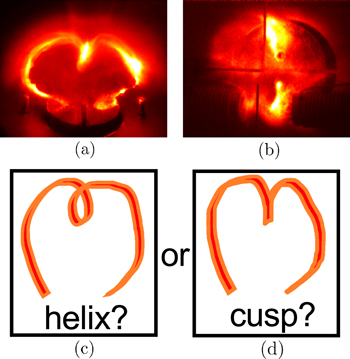
Figure 1. (a) Side view of lab experiment flux rope showing dip at the apex. (b) Top view of lab flux rope showing no evidence of helical shape. (c) Sketch of side view for helix interpretation. (d) Sketch of side view for downward cusp interpretation.
Download figure:
Standard image High-resolution imageThis paper identifies a formation mechanism for the cusp shape that is sketched in Figure 1(d) and provides detailed evidence from theory, experiment, and simulation that supports the cusp interpretation. The proposed mechanism is that neutral gas, injected from fast-gas valves (FGVs) at both footpoints, collides at the loop midplane creating a density pileup region. This causes the loop apex to have a greater linear mass density than the rest of the loop and, since the apex and the rest of the loop experience equivalent forces, the apex will have a slower acceleration, leading to the formation of a downward cusp during expansion. This theory explains why the dip is always downward, why there is no helical structure or dip growth, and why the feature only appears in experiments with gas injection from both footpoints. The results indicate that density perturbations can greatly distort the shape of an erupting flux rope and that introducing such perturbations may suppress external kink modes. These results are applicable to all MHD flux ropes with density perturbations (solar prominences, tokamaks, astrophysical jets, etc.) and are especially relevant to the morphology of solar eruptions. Furthermore, other plasma experiments that use FGVs (Hansen & Bellan 2001; Milanese et al. 2006; Stenson & Bellan 2012; Suzuki-Vidal et al. 2013; Onchi et al. 2014; Raman et al. 2014; Tenfelde et al. 2014; Loebner et al. 2015; Ha & Bellan 2016) should be aware of the potential for nonlinear interaction between multiple gas valves.
2. Experimental Apparatus
Experiments simulating solar flux ropes all share certain systems: a vacuum chamber, gas supply systems, solenoids, and electrodes. Each of these systems replicates a fundamental property of solar flux ropes: a vacuum chamber and a controlled gas supply are needed to create plasma of appropriate density, the solenoids recreate the background magnetic fields, and the electrodes drive current through the flux rope, adding the appropriate twist to the magnetic field.
2.1. Caltech Single-loop Experiments
The primary experiments of interest are the different iterations (Hansen & Bellan 2001; Stenson & Bellan 2012; Ha & Bellan 2016) of the Caltech single-loop experiment. All of these experiments exhibit the apex dip feature and have similar designs. The latest incarnation of the Caltech single-loop experiment (Ha & Bellan 2016) has a single pair of electrodes with internal solenoids and FGVs (Yee 1999). The system is mounted at the end of a 1.5 m long, 0.92 m diameter vacuum chamber with 10−7 Torr base pressure. The solenoids, located behind the electrodes, generate an arched background magnetic field ( ). Fast valves then release cones of neutral particles over 5 ms (Yun 2008) through holes in the electrodes into the vacuum chamber. High voltage applied to the electrodes by a 59 μF capacitor ionizes the gas to form an arched plasma of density n ∼ 1021 m−3. The capacitor is typically charged to 2.5–5 kV, driving 30 kA of current for 10 μs. The schematic diagram of the experimental setup is shown in Figure 2.

Figure 2. Schematic diagram of the experimental setup showing cones of neutral gas (blue) ejected from holes in the electrodes (copper), plasma loop (red), solenoids (green) providing background magnetic field, and gas injection system.
Download figure:
Standard image High-resolution image2.2. Other Experiments
The FlareLab experiment at Ruhr University Bochum was designed based on the Caltech apparatus, and has similar gas supply, timescales, electrodes, and magnetic fields (Tenfelde et al. 2014). This experiment also observes a downward apex dip.
The Princeton Plasma Physics Lab (PPPL) apparatus is located in the MRX facility (Myers et al. 2016). It uses uniform background gas injection as well as fast-gas valve injection at a single footpoint. Plasma is also generated via high voltage breakdown from the electrodes. However, the timescale for this experiment is ∼1 ms, one hundred times longer than the Caltech loop, and is comparable to the gas diffusion time. This experiment does not observe apex dips.
The UCLA single-loop experiment (Tripathi & Gekelman 2013) is generated in a uniform pre-ionized plasma and utilizes LaB6 electrodes with much lower currents (600 A). Additional density is added from laser ablation of targets at the footpoints to trigger eruptions. No apex dips are observed in this experiment either.
For comparison, Figure 3 shows the white light images for the solar flux rope in all four experiments.
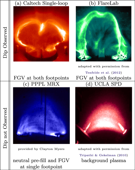
Figure 3. Comparison of white light images for arched flux rope experiments with their gas supply. Only experiments with FGVs at both footpoints observe a dip feature.
Download figure:
Standard image High-resolution image3. Theory
3.1. Single Gas Valve
The Caltech experiment has detailed measurements of the neutral density profile emerging from a single footpoint (Yun 2008; Moser 2012). This measured profile is that of an exponential cone:
where  ,
,  is the half cone angle, z0 = 0.01 m, and
  is the density at the footpoints.
3.2. Two Gas Nozzles
The two gas nozzles (1 cm apertures) are equally spaced in the y direction ( cm) and point in the z direction. This gas injection from both nozzles creates overlapping gas cones. If the mean free path is large, the neutral gas in the two cones will not interact and the final distribution is simply a linear superposition of the two cones (Figure 4(a)). However, if the neutral gas has a mean free path comparable to the system size (∼10 cm), the gases will interact and a density pileup will form between the two cones. The mean free path is defined as
  , where σ is the cross section and n is the number density. Calculations of
  for the three main gases used in the experiment are shown in Table 1.
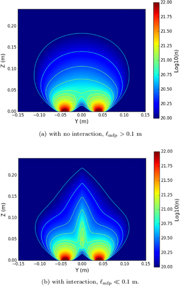
Figure 4. Density profiles for (a) direct superposition of two gas cone profiles and (b) modeled gas profile with finite neutral mean free path (Equation (2)).
Download figure:
Standard image High-resolution imageTable 1. Parameters for Density Pileup
| H2 | He | N2 | |
|---|---|---|---|
| n (m−3) | 1020–1021 (Moser 2012) | 1020–1021 (Moser 2012) | 1020–1021 (Moser 2012) |
| σ (10−19 m2) | 2.62 (Ismail et al. 2015) | 2.35 (Matteucci et al. 2006) | 4.16 (Ismail et al. 2015) |
 (m) (m) |
0.0027–0.027 | 0.003–0.03 | 0.0017–0.017 |
Download table as: ASCIITypeset image
Under standard experimental conditions, all three gases have a mean free path less than 3 mm. Since the overlap region is several centimeters wide, there should be significant interaction between the two cones.
3.3. Pileup Region Model
Estimating the extent and magnitude of the pileup involves evaluating how the density from cone 1 penetrates into cone 2. To first order, this pileup should be confined to the scale of the mean free path,  , and conserve mass. To satisfy these basic constraints, the pileup model is constructed such that the interpenetrating density is compressed to an exponential profile with local characteristic length
  :
:

This corresponds to integrating the density from cone 1 (e.g., left cone at  ), which penetrates the XZ-plane at each height, and redistributing it in an exponential profile with characteristic length
  . The process is mirrored for cone 2.
The estimated density pileup from this exponential profile increases the apex density by a factor of 1.6, relative to the noninteracting case. Figure 4 highlights the difference between the case of no interaction,  m, and the pileup region model,
  m. A pileup region creates peaked density contours as distinct from the flat profile of a direct superposition. For the gas cones and densities described here, this model predicts that the pileup effect is only significant for valve separation distances less than 12 cm.
Although this is an ad hoc model, 2D measurements of the FlareLab initial density profile (Tenfelde et al. 2012; Mackel 2014; Mackel et al. 2015) show a peaked density distribution, with contours very similar to those of Figure 4(b), indicating a comparable pileup region at the loop apex. This pileup model is used in Section 5 for the initial conditions of a 3D MHD simulation of the experiment.
3.4. Hoop Force
The hoop force is an outward radial force present in all curved current channels. This force exists because the internal magnetic pressure of a current loop is greater than the exterior magnetic pressure. The equation of motion for an infinitesimal segment of a circular current (length ds, major radius R, minor radius a, and average mass density  ) is given by

where I is the current flowing through the plasma loop, and li is a constant of order unity related to the internal current distribution (Stenson & Bellan 2012; Ha & Bellan 2016). Approximating the term in square brackets in Equation (5) as constant and assuming a linearly rising current, the major radius expands quadratically with time:  (Stenson & Bellan 2012). However, sections of the loop with higher density will accelerate more slowly and lag behind the global expansion.
4. Experimental Results
Several observed features on the Caltech experiment indicate the presence of a density pileup at the loop apex. The first of these is the presence of a localized bright region at the loop apex; this bright region can be detected from fast camera images as early as 500 ns after the breakdown. Since the apex is 6 cm away from each footpoint, the plasma at the footpoints does not have time to travel to the apex in 500 ns ( m s−1, 6 cm/vA = 2 μs). Consequently, this feature must already be present in the neutral density. Figure 5 shows an image of this bright apex feature for a Nitrogen loop 1.5 μs after breakdown. This bright feature at the loop apex extends beyond the major radius in an expanding cone. This expansion of the pileup region width at greater heights is consistent with the increasing mean free path further away from the fast-gas nozzles.

Figure 5. Photograph of the loop at 1.5  after breakdown. The white dashes mark the bright feature at the loop's apex and pileup cone at the midplane.
Download figure:
Standard image High-resolution imageThe second observation is that the loop apex always lags behind during expansion, forming a heart-shaped dip. This expansion is driven by the hoop force described in Section 3.4. This dip is unusual as it is a large, extremely reproducible feature. It is always pointed downward, remains a similar size, and appears consistently for all gases used (H2, He, Ar, and N2). The dip moves slower than the leading edge of the loop and creates a significant deformation from circular expansion. Figure 6(a) shows the evolution of this apex dip for a N2 loop.
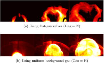
Figure 6. Plot shows the evolution of two different initial density profiles. (a) Standard initial conditions with two colliding cones of gas supplied by the nozzles in the electrodes. (b) Non-standard conditions with uniform background gas supplied from sources on the opposite side of the chamber. Without the gas cones from the nozzles, the apex dip feature disappears.
Download figure:
Standard image High-resolution imageWe can also control the shape and location of this apex dip by varying the gas output of each FGV. For the symmetric gas output, the dip appears to be sharper and larger when the gas density output is higher, as shown in Figure 7. If the output of the FGVs differ significantly, the pileup region is shifted away from the footpoint with greater gas output and toward the footpoint with weaker gas output. Figure 8 shows superimposed images of a shot with higher gas output on the right footpoint (red) and a shot with higher gas output on the left footpoint (cyan). The shift of the bright apex feature is about 3 cm and highly reproducible.
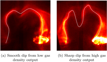
Figure 7. Comparison of dip shape for two different gas outputs. The loop axis is manually traced with white lines to highlight differences (Gas = H).
Download figure:
Standard image High-resolution image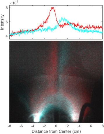
Figure 8. (top) Plot of vertically integrated pixel values. (bottom) Superimposed images of a shot (red) with higher gas output on the right footpoint and a shot (cyan) with higher gas output on the left footpoint (gas = He).
Download figure:
Standard image High-resolution imageLastly, when creating plasma loops from a uniform gas backfill, both the bright apex feature and the heart shape are not observed. Figure 6(b) shows the evolution of a loop created with uniform Hydrogen backfill.
These observations demonstrate that the apex dip depends strongly on the initial neutral gas profile.
5. Ideal MHD Simulation
Simulations of density profiles with a pileup region were performed to confirm that this perturbation would reproduce the shape and velocity of the experimental loop. The simulations were performed using the 3D MHD equations solver code, a subset of the Los Alamos COMPutational Astrophysics Simulation Suite (LA-COMPASS; Li & Li 2003). This code has been used to simulate AGN jets in the intra-cluster medium (Li et al. 2006) and the Caltech plasma jet experiment (Zhai et al. 2014). The spatial domain is a mesh cube with 96 grid points in each Cartesian dimension and non-reflecting outflow boundary conditions. The code evolves a set of two 3D vectors (velocity, magnetic field) and two scalars (density, pressure) at each grid point through the system of dimensionless ideal MHD equations listed below.


The total energy, (e), is defined by  ,
,  . To simulate helicity injection from the electrodes, a poloidal magnetic field corresponding to the measured current is injected into the system.
5.1. Initial Conditions
The simulation uses the initial density profile shown in Figure 4. In addition to the two gas cones, a high-density wall region is added below the footpoints to simulate the anchoring effects of the electrodes.
The initial background magnetic field (bias field) is generated by specifying a set of loop currents in a half-circle configuration below the electrode plane. This ensures that all field lines emerge and terminate at the footpoints. This topology is closer to that of the experimental field (i.e., where Bz does not change sign on a given electrode) than a simple dipole and is scaled to match the measured field strength at the loop apex. The resulting initial bias field is shown in Figure 9.
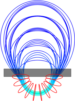
Figure 9. Plot of the initial conditions for the simulation. Source currents for the background magnetic field consist of 10 thin loops arranged in a semi-circle (red), B-field lines are shown in blue. The high-density plasma wall boundary is shown in black.
Download figure:
Standard image High-resolution image5.2. Current Injection
Diffuse poloidal flux is continuously injected into the simulation domain corresponding to the electric current measured in the experiment. The diffuse current profile is constructed from the superposition of 110 thin circular current loops, where each loop has a simple analytic magnetic field expression (Simpson et al. 2001). To avoid singularities, the elliptic integrals are approximately evaluated using a truncated power series. This injected distribution, shown in Figure 10(a), is physically motivated by experimental current density measurements that indicate that the current profile begins as a flared diffuse structure and maintains this outer diffuse current during helicity injection. Figure 10(c) shows the current path of 10 loops in yz-plane with apexes equally spaced from  to
to  . Figure 10(b) shows another view of the profile in xz-plane with 11 sets of 10 current loops distributed over
 ![${\theta }_{{yz}}\in [-54^\circ ,54^\circ ]$](https://content.cld.iop.org/journals/0004-637X/848/2/89/revision1/apjaa8990ieqn23.gif) , with respect to the yz-plane. The injected current profile is stationary throughout the simulation. Since we are principally interested in the formation phase, we do not attempt to model the helicity extraction or the decreasing current after
, with respect to the yz-plane. The injected current profile is stationary throughout the simulation. Since we are principally interested in the formation phase, we do not attempt to model the helicity extraction or the decreasing current after  μs. The experimentally measured current undergoes a damped oscillation with a period of T = 40 μs, so we model the temporal dependence of the injection as

where  has only spatial dependency and H is a heaviside step function.

Figure 10. Illustration of spatial profile of the current injection. Each red circle represents a thin circular current loop. (a) The 3D view showing all 110 loops. (b) The 2D cross section in the xz-plane. (c) The 2D cross section in the yz-plane. The spatial units are in centimeters.
Download figure:
Standard image High-resolution image5.3. Simulation Results
Using an initial density with a pileup region, the simulation replicates the shape and expansion velocity of the loop. Figure 11(a) shows the image of the loop with the dip at the apex, and Figure 11(b) shows a synthetic image from the simulation where intensity is proportional to current density and number density squared ( ). Figure 12 shows that the apex position of the simulated loop also closely matches that of the experiment. The evolution comprises of three stages. First, after the initial brightening of neutral gas as shown in Figure 5, magnetic forces generate axial flow and pinch to form a collimated loop (Bellan 2003), resulting in the initial decrease in apex height. Subsequently, the apex is accelerated by the hoop force (Stenson & Bellan 2012), colliding with the neutral pileup region. Lastly, the apex is accelerated to its terminal velocity from the high magnetic curvature forces, illustrated in Figure 13, present in the cusp.

Figure 11. Comparison of the cusp shape between experiment (left) and simulation (right).
Download figure:
Standard image High-resolution image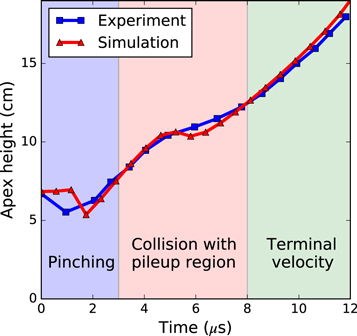
Figure 12. Evolution of the loop apex position in 3 stages. (i) The minor radius undergoes pinching before expansion. (ii) The loop collides with the pileup region and temporarily slows down. (iii) The magnetic curvature forces of the cusp re-accelerate the apex to a terminal velocity.
Download figure:
Standard image High-resolution image
Figure 13. Magnetic tension forces ( , arrows) plotted for an apex dip of a thin flux rope (blue line). The central cusp area has strong vertical magnetic forces because of the high curvature.
Download figure:
Standard image High-resolution image
Given the good match in shape and velocity, the simulation demonstrates that a pileup region is consistent with the observed loop evolution.
6. Discussion
The data presented provide strong evidence that the dip feature is in fact a cusp rather than a helix. The proposed cusp formation mechanism, a neutral pileup region, resolves all of the inconsistencies with the helical interpretation and achieves excellent agreement with observation and simulation. This new understanding of the experiment has implications for both future experiments and solar flux ropes.
6.1. Neutral Pileup Regions
Most other experiments with FGVs do not have the appropriate densities or length scales necessary to create density pileup regions. However, as in our experiments, such an effect can greatly perturb the initial conditions and should be considered in the design of future plasma experiments. The high reproducibility and simple control of the feature suggests that future experiments could utilize such pileup regions to study the effect of density perturbations, instabilities, or localized collisions between plasma and neutral gas.
6.2. Relevance of Dip Feature in Solar Context
Since the plasma loop can be described by ideal MHD, its behavior can be scaled. This scaling allows for three free parameters a1, a2, and a3 with the following invariant transformations:  ,
,  ,
,  ,
,  ,
,  ,
,  , and
, and  (Ryutov et al. 2000). These transformations provide a one-to-one correspondence between systems, allowing simulated and experimental plasmas to be scaled to an equivalent system at the space plasma scale. Table 2 shows the characteristic parameters of the experiment, typical coronal loop parameters, and experimental parameters scaled to the solar environment using
  ,
,  , and
, and  . With the notable exception of gravity, the experimental parameters scale well to the solar case. However, the effective gravity associated with the acceleration provides useful insight into gravitational effects.
Table 2. Dimensionless Scaling of Caltech Parameters to Solar Loops
| Experiment | B = 3000 G | L = 0.5 m |
| ρ = 10−4 kg m−3 | τ = 20 μs | |
| g = 10 m s−2 | P = 300 Pa | |
| vA = 3 × 10⁴ m s−1 | β = 0.01 | |
| Scaled Exp. | B = 30 G | L = 2 × 10⁷ m |
| ρ = 10−12 kg m−3 | τ = 7 s | |
| g = 3 × 10⁻³ m s−2 | P = 0.03 Pa | |
| vA = 3 × 10⁶ m s−1 | β = 0.01 | |
| Coronal Loop | B = 50 G | L = 2 × 10⁷ m |
| T = 1.5 MK | ρ = 10−12 kg m−3 | τ = 5 s |
| g = 300 m s−2 | P = 0.01 Pa | |
| vA = 4 × 10⁶ m s−1 | β = 0.002 | |
Download table as: ASCIITypeset image
The presence of a dense, cusp feature in the experimental flux rope is similar to common features of solar prominences. It is well established that solar prominences have inhomogeneous density along their axis and that the highest density is localized near the apex (Patsourakos & Vial 2002; Labrosse et al. 2010; Arregui & Soler 2015). Despite these measurements of density modulation, many models of coronal structures assume constant density (Tokman & Bellan 2002; Arnold et al. 2008; Wiegelmann & Sakurai 2012; Jiang et al. 2014; Inoue 2016). The experimental results indicate that density perturbations can result in large distortions of an erupting flux rope, even in the absence of significant pressure or gravitational forces. Consequently, a more realistic density profile should be considered when attempting to precisely model erupting flux ropes or coronal mass ejections.
Furthermore, this denser apex material is thought to sit in a shallow magnetic dip (Heinzel & Anzer 1999; Gunár et al. 2013), a similar but less extreme version of the experimental cusp. Many of the models simulating this apex density are purely hydrodynamic (Antiochos et al. 2000) and ignore magnetic effects from changes in minor radius. In future experiments, these theories could be tested by appropriate acceleration of the loop apex, imposing an effective gravity with appropriate scaling to solar gravity. The acceleration from loop expansion with current parameters (5·107 m s−2) scales to an effective gravity of 104 m s−2 at the coronal scale, 40 times larger than solar gravity (270 m s−2).
6.3. Suppression of Kink Instability
The last mechanism of interest is the effect of the pileup region on the kink instability. The kink instability is a current-driven instability that drives exponential growth of long-wavelength helical perturbations. The instability threshold is reached when the magnetic field lines complete more than one twist around the major axis. The kink stability is usually defined with respect to the safety factor, q:
where q is the safety factor, L is the length of the major axis, a is the minor radius, Bϕ is the toroidal field, and Bθ is the poloidal field. Full toroids and other line-tied flux rope experiments (Bergerson et al. 2006; Oz et al. 2011) become unstable for  . B-field measurements of the loop from t = 10–14 μs give
  G, a = 2–4 cm. From images we know that the length of the loop is between 40–56 cm in this time frame. These values imply an unstable safety factor of
  . Consequently, it is surprising that the loop does not exhibit more violent kinking behavior.
We propose that the high-density region at the loop apex suppresses the kink since the unstable kink mode has an anti-node at the apex, and the high-density region acts like a stationary node. This effectively halves the axial length available to kink and doubles the safety factor. Similar suppression of the longest wavelength kink modes by high-density regions has been seen before in astrophysical jet simulations (Nakamura et al. 2001) and experiments (Hsu & Bellan 2003).
This work was supported by NSF under award 1348393, AFOSR under award FA9550-11-1-0184, and DOE under awards DE-FG02-04ER54755 and DE-SC0010471. H.L. and S.L. acknowledge the support from DoE/OFES and LANL/LDRD programs.