


Abstract
We present our ALMA multi-transition molecular line observational results for the ultraluminous infrared galaxy IRAS 20551−4250, which is known to contain a luminous buried active galactic nucleus and shows detectable vibrationally excited (v2 = 1f) HCN and HNC emission lines. The rotational J = 1–0, 4–3, and 8–7 of HCN,  , and HNC emission lines were clearly detected at a vibrational ground level (v = 0). Vibrationally excited (v2 = 1f) J = 4–3 emission lines were detected for HCN and HNC, but not for
  . Their observed flux ratios further support our previously obtained suggestion, based on J = 3–2 data, that (1) infrared radiative pumping plays a role in rotational excitation at v = 0, at least for HCN and HNC, and (2) HCN abundance is higher than
  and HNC. The flux measurements of the isotopologue H13CN,
  , and HN13C J = 3–2 emission lines support the higher HCN abundance scenario. Based on modeling with collisional excitation, we constrain the physical properties of these line-emitting molecular gases, but find that higher HNC rotational excitation than HCN and
  is difficult to explain, due to the higher effective critical density of HNC. We consider the effects of infrared radiative pumping using the available 5–30 μm infrared spectrum and find that our observational results are well-explained if the radiation source is located at 30–100 pc from the molecular gas. The simultaneously covered very bright CO J = 3–2 emission line displays a broad emission wing, which we interpret as being due to molecular outflow activity with the estimated rate of
  .
.
Export citation and abstract BibTeX RIS
1. Introduction
The ubiquity of supermassive black holes (SMBH) at the center of galactic stellar spheroidal components, and the mass correlation between SMBHs and spheroidal stars suggest that SMBHs are an important ingredient of galaxies (Magorrian et al. 1998; Ferrarese & Merritt 2000; Gultekin et al. 2009; McConnell & Ma 2013). In the current widely accepted galaxy formation scenario based on cold dark matter, small gas-rich galaxies collide and merge, and then grow into more massive galaxies (White & Rees 1978). Numerical simulations of such merging processes of gas-rich galaxies containing SMBHs at their centers have been extensively performed, and it has been argued that active star formation and mass accretion onto central SMBHs occur in highly obscured regions during an infrared luminous phase (Hopkins et al. 2005, 2006, 2008; Debuhr et al. 2011).
Active mass accretion onto SMBHs emits strong radiation and is observed as active galactic nucleus (AGN) activity. Luminous AGNs deeply buried in gas/dust-rich infrared luminous merging galaxies are now thought to play an essential role in galaxy formation, through feedback to galaxies (Granato et al. 2004; Di Matteo et al. 2005; Springel et al. 2005; Robertson et al. 2006; Sijacki et al. 2007; Hopkins et al. 2008; Ciotti et al. 2010); however, observational understanding of such buried AGNs is not easy, due to dust extinction. We must establish a method to detect and investigate the properties of buried AGNs by separating these from the surrounding starburst emission. Observing at wavelengths where the effects of dust extinction are small is clearly one of the best ways to study dust-obscured energy sources.
Molecular rotational J-transition emission line flux ratios at the (sub)millimeter wavelength can be a powerful tool to study buried energy sources because: (1) dust extinction is typically negligible, unless the column density of obscuring material is very high (e.g.,  cm−2); and (2) some molecular lines are argued to become good signatures of AGN activity. In particular, molecules with high dipole moments, such as HCN, HCO+, and HNC, are better suited than the widely used low-J transition CO emission lines to investigate physical properties around hidden energy sources, because nuclear molecular gas in the vicinity of active star formation and AGN activity is usually in a dense form with >104 cm−3. For example, it was proposed that optically selected AGNs and starbursts show different molecular line flux ratios, in such a way that, in AGNs, HCN rotational J-transition emission lines are enhanced relative to HCO+ (Kohno 2005; Krips et al. 2008). Based on pre-ALMA and ALMA observations of the nuclei of gas/dust-rich luminous infrared galaxies (LIRGs; infrared luminosity LIR > 1011 L⊙), which are diagnosed to contain optically detectable AGNs, or AGNs that are optically elusive (but detectable by infrared/X-ray), or else no detectable AGNs, it was demonstrated that (sub)millimeter molecular emission line flux ratios indeed work to detect the signs of deeply buried AGNs in these LIRGs (Imanishi et al. 2004, 2006, 2007, 2009, 2016a, 2016b, 2016c; Imanishi & Nakanishi 2006, 2013a, 2013b, 2014; Costagliola et al. 2011; Iono et al. 2013; Izumi et al. 2015, 2016; Privon et al. 2015). Thus, these (sub)millimeter molecular line observations have potential in the systematic investigation of buried AGNs in gas/dust-rich LIRGs, not only in the local universe, but also in the distant universe, thanks to the advent of the highly sensitive ALMA observing facility in this wavelength range.
However, the physical origin of the strong HCN J-transition line emission in AGNs remains to be fully understood. An HCN abundance enhancement in molecular gas in the close vicinity of a buried AGN is a natural explanation for the strong HCN emission (Yamada et al. 2007; Izumi et al. 2016). While this scenario of high HCN abundance in molecular gas, largely affected by AGN radiation, is predicted in some parameter ranges by chemical calculations (Meijerink & Spaans 2005; Lintott & Viti 2006; Harada et al. 2010), it is not necessarily true that the HCN abundance is always higher than HCO+ around an AGN (Meijerink & Spaans 2005; Harada et al. 2013). Higher HCN rotational J-excitation in an AGN than in a normal starburst is an alternative explanation, because the AGN's higher radiative energy generation efficiency can increase the temperature of the surrounding molecular gas—and it can excite HCN (which has higher critical density than HCO+ under the same line opacity) more than in a normal starburst (Imanishi et al. 2016c). Multiple rotational J-transition line observations are required to disentangle the abundance and excitation effects (Imanishi et al. 2016c). Flux attenuation by line opacity (not dust extinction) is another uncertain factor when discussing the hidden energy sources based on observed molecular line flux ratios (Costagliola et al. 2015). Optically thin isotopologue molecular line observations will help us to estimate these line opacity effects for the main bright molecular emission lines.
Vibrationally excited molecular emission lines with energy levels much higher than the widely investigated rotationally excited emission lines at a vibrational ground level (v = 0) may potentially be another good AGN indicator. The vibrationally excited (v2 = 1, l = 1f; hereafter v2 = 1f) emission lines of HCN and HNC have recently been detected in several LIRGs (Sakamoto et al. 2010; Imanishi & Nakanishi 2013b; Aalto et al. 2015a, 2015b; Costagliola et al. 2015; Imanishi et al. 2016b, 2016c; Martin et al. 2016). Because the energy levels of these vibrationally excited states are ∼1030 K (670 K) for HCN (HNC), they are very difficult to excite by collision; however, an infrared radiative pumping process can achieve this by absorbing ∼14 μm (∼22 μm) infrared photons (Aalto et al. 1995; Sakamoto et al. 2010). Because an AGN can emit mid-infrared (3–30 μm) continuum emission more efficiently than a starburst with the same bolometric luminosity, due to AGN-heated hot (>100 K) dust emission, if the vibrationally excited emission lines are strongly detected in LIRGs, then an obscured AGN is a plausible origin of the strong infrared continuum emission that vibrationally excites HCN and HNC (Aalto et al. 2015a). However, an extreme starburst with a very compact size remains another possibility (Aalto et al. 2015a).
The ultraluminous infrared galaxy (ULIRG) IRAS 20551−4250, with infrared luminosity  at z = 0.043 (Table 1), is one such galaxy where vibrationally excited (v2 = 1f) HCN and HNC emission lines have been clearly detected, due to small observed molecular line widths (Imanishi & Nakanishi 2013b; Imanishi et al. 2016b). The observed HCN-to-HCO+ flux ratios at J = 3–2 and J = 4–3 have been found to be substantially larger than in starburst-dominated regions (Imanishi & Nakanishi 2013b; Imanishi et al. 2016b). This galaxy displays a long merging tail in the southern direction from the main single nucleus (Duc et al. 1997; Rothberg & Joseph 2004). Based on optical emission line flux ratios, it is classified as a LINER/H ii-region (Duc et al. 1997), whereas Yuan et al. (2010) classified it as a starburst-AGN composite or H ii-region type, depending on the emission lines used. The presence of a buried AGN, which could explain 20%–60% of the bolometric luminosity, has been suggested in addition to starburst activity, based on infrared and X-ray observations (Franceschini et al. 2003; Risaliti et al. 2006; Nardini et al. 2008, 2009, 2010; Sani et al. 2008; Imanishi et al. 2010, 2011; Veilleux et al. 2013). Because IRAS 20551−4250 displays bright molecular rotational J-transition emission lines (Imanishi & Nakanishi 2013b; Imanishi et al. 2016b), this is an interesting and valuable object to improve our understanding of the physical origin of observed molecular emission line properties, based on multiple rotational J-transition lines for multiple molecules.
Table 1. Observed Properties of IRAS 20551−4250
| Object | Redshift |

|

|

|

|
log 
|
log 
|

|
q |
|---|---|---|---|---|---|---|---|---|---|
| (Jy) | (Jy) | (Jy) | (Jy) | ( ) ) |
( ) ) |
(mJy) | |||
| (1) | (2) | (3) | (4) | (5) | (6) | (7) | (8) | (9) | (10) |
| IRAS 20551−4250 | 0.043 | 0.28 | 1.91 | 12.78 | 9.95 | 12.0 | 11.9 | 31.0 | 2.7 |
Note. Column (1): Object name. Column (2): Redshift. Columns (3)–(6): f12, f25, f60, and f100 are IRAS fluxes at 12 μm, 25 μm, 60 μm, and 100 μm, respectively, taken from the IRAS FSC catalog. Column (7): Decimal logarithm of infrared (8–1000 μm) luminosity in units of solar luminosity ( ), calculated with
  D(Mpc)2 × (
 ) (erg s−1) (Sanders & Mirabel 1996). Column (8): Decimal logarithm of far-infrared (40–500 μm) luminosity in units of solar luminosity (
 ), calculated with
  D(Mpc)2 × (
 ) (erg s−1) (Sanders & Mirabel 1996). Column (9): Radio 1.4 GHz flux in (mJy) (Condon et al. 1996). Column (10): Decimal logarithm of the far-infrared-to-radio flux ratio, defined as a q-value (Condon et al. 1991).
Download table as: ASCIITypeset image
In this study, we present our new ALMA observational results in bands 3 (84–116 GHz), 7 (275–373 GHz), and 9 (602–720 GHz) of the ULIRG, IRAS 20551−4250. The J = 1–0, J = 4–3, and J = 8–7 emission lines of HCN, HCO+, and HNC are covered in bands 3, 7, and 9, respectively. For J = 4–3, vibrationally excited (v2 = 1f) emission lines were also observed for HCN, HCO+, and HNC. For J = 8–7, vibrationally excited (v2 = 1f) HCN and HNC emission lines were included in our band 9 data.4
ALMA band 6 (211–275 GHz) observations of isotopologue lines, H13CN, H13CO+, and HN13C J = 3–2, were also conducted and their results are included. We adopt H0 = 71 km s−1 Mpc−1,  , and
, and  (Komatsu et al. 2009), to be consistent with our previously published ALMA papers for this galaxy. The physical scale at
  is 0.84 kpc arcsec−1. In the absence of a statement about vibrational level, we mean the vibrational ground level (v = 0).
2. Observations and Data Analysis
Band 7 (275–373 GHz), 3 (84–116 GHz), 9 (602–720 GHz), and 6 (211–275 GHz) observations were conducted through our ALMA Cycle 2 program 2013.1.00033.S (PI = M. Imanishi), Cycle 3 program 2015.1.00028.S (PI = M. Imanishi), Cycle 3 program 2015.1.00028.S (PI = M. Imanishi), and Cycle 4 program 2016.1.00051.S (PI = M. Imanishi), respectively. The widest 1.875 GHz band mode and 3840 total channel number were employed for all observations. To reduce the data rate, online spectral averaging with a factor of 2 or 4 was applied for some observations. Table 2 summarizes these ALMA observations.
Table 2. Log of Our ALMA Observations
| Band | Date | Antenna | Baseline | Integration | Calibrator | ||
|---|---|---|---|---|---|---|---|
| (UT) | Number | (m) | (minutes) | Bandpass | Flux | Phase | |
| (1) | (2) | (3) | (4) | (5) | (6) | (7) | (8) |
| Band-7a (HCO+ J = 4–3) | 2014 Jun 8 | 34 | 28–646 | 15 | J1924−2914 | Titan | J2056−4714 |
| 2015 Apr 3 | 37 | 15–328 | 15 | J1924−2914 | Titan | J2056−4714 | |
| Band-7b (HNC J = 4–3) | 2014 Jun 8 | 34 | 28–646 | 39 | J1924−2914 | J2056−4714 | J2056−4714 |
| 2015 Apr 29 | 39 | 15–349 | 39 | J2056−4714 | Titan | J2056−4714 | |
| Band 9 (HCN, HCO+, and HNC J = 8–7) | 2016 May 18 | 42 | 15–640 | 39 | J2253+1608 | Pallas | J2056−4714 |
| Band-3 (HCN, HCO+, and HNC J = 1–0) | 2016 May 27 | 41 | 15–784 | 39 | J2056−4714 | J2056−4714 | J2049−4020 |
| 2016 Aug 15 | 38 | 15–1462 | 47 | J2056−4714 | J2056−4714 | J2049−4020 | |
| Band-6 (H13CN, H13CO+, HN13C J = 3–2) | 2016 Oct 1 | 41 | 15–3248 | 40 | J1924−2914 | J2056−4714 | J2056−4714 |
| 2016 Oct 5 | 44 | 19–3248 | 40 | J2056−4714 | J2056−4714 | J2056−4714 | |
| 2016 Oct 5–6 | 44 | 19–3248 | 40 | J2056−4714 | J2056−4714 | J2056−4714 | |
Note. Column (1): Observed band and primarily targeted emission lines. Column (2): Observing date in UT. Column (3): Number of antennas used for observations. Column (4): Baseline length in meters. Minimum and maximum baseline lengths are shown. Column (5): Net on-source integration time in minutes. Columns (6)–(8): Bandpass, flux, and phase calibrators for the target source, respectively.
Download table as: ASCIITypeset image
For our ALMA band 7 observations, we covered HCO+ J = 4–3 (rest-frame frequency is  GHz), HCN v2 = 1f J = 4–3 (
 GHz), and HCO+ v2 = 1f J = 4–3 (
 GHz), but had to exclude the HCN J = 4–3 line (
 GHz), due to the limited frequency coverage of the ALMA system. HCN J = 4–3 and HCO+ J = 4–3 (v = 0) lines were observed in our ALMA Cycle 0 observations (Imanishi & Nakanishi 2013b). The bright HCO+ J = 4–3 (v = 0) emission line can be used for inter-calibration between Cycle 0 and 2 data by correcting for possible absolute flux calibration uncertainty during individual ALMA observations. The very bright CO J = 3–2 (
 GHz) emission line was also included in our Cycle 2 observations. HNC J = 4–3 emission lines at v = 0 (
 GHz) and v2 = 1f (
 GHz) were obtained independently from the HCO+ J = 4–3 observations.
For band 9, HCN J = 8–7 ( GHz), HCO+ J = 8–7 (
 GHz), and HNC J = 8–7 (
 GHz) lines were observed. The vibrationally-excited HCN v2 = 1f J = 8–7 (
 GHz) and HNC v2 = 1f J = 8–7 (
 GHz) lines were also covered, but HCO+ v2 = 1f J = 8–7 (
 GHz) line was not. Our scientific aim was to measure the strengths of the vibrational ground (v = 0) J = 8–7 emission lines of HCN, HCO+, and HNC; vibrationally excited (v2 = 1f) emission lines were our second objective.
In bands 7 and 9, vibrationally excited (v2 = 1, l = 1e; hereafter v2 = 1e) J = 4–3 and J = 8–7 lines, respectively, were covered for HCN, HCO+, and HNC. However, these frequencies are so close to the bright vibrational ground (v = 0) emission lines for HCN, HCO+, and HNC that we could not extract the faint v2 = 1e emission line components in a reliable manner. These v2 = 1e emission line fluxes will not be discussed in this paper.
For band 3, HCN J = 1–0 ( GHz), HCO+ J = 1–0 (
 GHz), and HNC J = 1–0 (
 GHz) line data were obtained.
For band 6, we targeted H13CN ( GHz), H13CO+ (
 GHz), and HN13C J = 3–2 (
 GHz), because these isotopologue emission lines are thought to be optically thin, and thus can be used to estimate possible flux attenuation by line opacity (not dust extinction) for the previously obtained HCN, HCO+, and HNC J = 3–2 emission lines (Imanishi et al. 2016b). The bright CS J = 5–4 line (
 GHz) was included in this band 6 observation.
We performed data analysis in the same way as for our previously obtained ALMA data of IRAS 20551−4250 (Imanishi & Nakanishi 2013b; Imanishi et al. 2016b). We retrieved data calibrated by ALMA, and used CASA (https://casa.nrao.edu) for further data reduction. For the spectral window that includes the very bright CO J = 3–2 emission line, we employed self-calibration, using the CO J = 3–2 emission line itself for phase calibration. Except for this spectral window, we adopted results produced with a standard phase calibration using phase calibrators, which were provided by ALMA. We first checked the visibility plots to view the signatures of bright emission lines. To estimate the continuum flux levels, we removed channels that contained discernible emission lines. We then subtracted the derived continuum levels, to extract only molecular line data. The task "clean" was then applied for the molecular line data by binning spectral channels to make the velocity resolution 20–40 km s−1. Pixel scale was set as 0 1 pixel−1 for band 3 and 7 data, but was 003 pixel−1 for band 9 and 6 data, because their beam sizes were much smaller than those of bands 3 and 7. The "clean" task was also applied for continuum data. We then obtained spectra at the nuclear position defined from the continuum peaks in individual observations. When the flux density levels in the spectra were significantly below zero at the frequency where no emission and/or absorption lines were expected to be present, continuum was over-subtracted, possibly due to the inclusion of weak emission lines for continuum determination. In such cases, we redefined line-free channels and created clean maps of molecular emission lines and continuum. After confirming that the extracted spectra at line-free channels at the continuum peak position show flux density fluctuating around zero level with noise, we adopted these re-analyzed results as final products.
3. Result
Continuum-J43a (taken with HCO+ J = 4–3), continuum-J43b (taken with HNC J = 4–3), continuum-J87 (taken with HCN, HCO+, and HNC J = 8–7), continuum-J10 (taken with HCN, HCO+, and HNC J = 1–0), and continuum-J32 (taken with H13CN, H13CO+, and HN13C J = 3–2) maps are displayed in Figure 1. In all maps, continuum emission is dominated by a spatially compact component at the nucleus of IRAS 20551−4250. Table 3 lists continuum fluxes at the peak position. We had two continuum measurements in band 7 with slightly different central frequencies ( GHz and 343.2 GHz; Table 3). Both of these provided comparable flux levels with 10.5 and 10.3 (mJy beam−1) (Table 3). Band 7 continuum measurements of IRAS 20551−4250 were made in ALMA Cycle 0, and the estimated fluxes were 10.1 (mJy beam−1) (
 GHz) and 9.4 (mJy beam−1) (
 GHz) (Imanishi & Nakanishi 2013b). These band 7 continuum measurements at similar central frequencies, taken in ALMA Cycles 0 and 2, agree within ∼10%, supporting the quoted <10% absolute flux calibration uncertainty in individual ALMA observations (ALMA Proposer's Guide for Cycles 0 and 2).
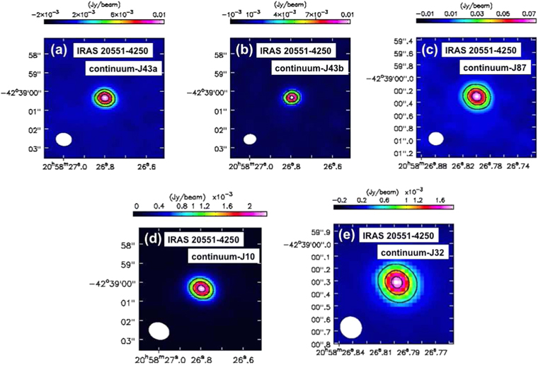
Figure 1. Continuum emission maps in bands 7, 9, 3, and 6. The abscissa and ordinate are R.A. (J2000) and decl. (J2000), respectively. (a) Continuum-J43a (central observed frequency  GHz) data taken with the HCO+ J = 4–3 observations in band 7. (b) Continuum-J43b (
 GHz) data taken with the HNC J = 4–3 observations in band 7. (c) Continuum-J87 (
 GHz) data taken with the HCN, HCO+, and HNC J = 8–7 observations in band 9. (d) Continuum-J10 (
 GHz) data taken with HCN, HCO+, and HNC J = 1–0 observations in band 3. (e) Continuum-J32 (
 GHz) data taken with H13CN, H13CO+, and HN13C J = 3–2 observations in band 6. The contours represent 20σ, 35σ, and 50σ for continuum-J43a; 25σ, 50σ, and 75σ for continuum-J43b; 8σ, 16σ, and 24σ for continuum-J87; 25σ, 40σ, and 55σ for continuum-J10; and 20σ, 40σ, and 60σ for continuum-J32. Beam sizes are shown as filled circles in the lower-left region. The displayed sizes in bands 9 and 6 are different from those of bands 7 and 3 because of smaller beam sizes in the former.
Download figure:
Standard image High-resolution imageTable 3. Continuum Emission Properties
| Continuum | Frequency | Flux | Peak Coordinate | rms | Synthesized Beam |
|---|---|---|---|---|---|
| (GHz) | (mJy beam−1) | (R.A., Decl.)J2000 | (mJy beam−1) | (arcsec × arcsec) (°) | |
| (1) | (2) | (3) | (4) | (5) | (6) |
| J10 | 84.1–87.9, 96.1–99.9 | 2.3 (61σ) | (20 58 26.80, −42 39 00.3) | 0.038 | 1.1 × 0.9 (68°) |
| J32 | 232.1–235.7, 247.3–250.9 | 1.8 (68σ) | (20 58 26.80, −42 39 00.3) | 0.027 | 0.18 × 0.17 (46°) |
| J43a | 329–332.5, 340.7–344.4 | 10.5 (59σ) | (20 58 26.80, −42 39 00.3) | 0.18 | 0.84 × 0.68 (82°) |
| J43b | 335.3–338.9, 347.2–351.0 | 10.3 (81σ) | (20 58 26.80, −42 39 00.3) | 0.13 | 0.66 × 0.53 (−81°) |
| J87 | 678.7–684.4, 694.2–701.0 | 75.7 (29σ) | (20 58 26.80, −42 39 00.3) | 2.6 | 0.23 × 0.21 (89°) |
Note. Column (1): Continuum. J10, J32, J43a, J43b, and J87 were taken with "HCN, HCO+, and HNC J = 1–0," "H13CN, H13CO+, and HN13C J = 3–2," "HCO+ J = 4–3," "HNC J = 4–3," and "HCN, HCO+, and HNC J = 8–7," respectively. Column (2): Observed frequency in (GHz). Column (3): Flux in (mJy beam−1) at the emission peak. The detection significance relative to the rms noise is shown in parentheses. Possible systematic ambiguity, coming from ALMA absolute flux calibration uncertainty and choice of frequency range for continuum determination, is not included. Column (4): The coordinate of the continuum emission peak in J2000. Column (5): The rms noise level (1σ) in (mJy beam−1). Column (6): Synthesized beam in (arcsec × arcsec) and position angle in (°). The position angle is 0° in the north–south direction and increases in the counter-clockwise direction.
Download table as: ASCIITypeset image
Spectra in bands 7, 9, 3, and 6 at the continuum peak positions within the beam size of individual data are presented in Figure 2. The targeted bright emission lines, such as the CO J = 3–2 line, the J = 8–7, J = 4–3, and J = 1–0 lines of HCN, HCO+, and HNC, and the J = 3–2 lines of H13CN, H13CO+, and HN13C were clearly detected. Additionally, signatures of several fainter emission lines, including v2 = 1f J = 4–3 emission lines of HCN, HCO+, HNC, and other serendipitously detected emission lines, were observed. Identifying the detected faint emission lines is not an easy task because gas-rich (U)LIRGs exhibit many faint emission lines from molecules, and the bulk of the observed frequency range could be occupied by such lines, particularly in band 7 (Costagliola et al. 2015). Our proposed identifications of faint emission lines are indicated with arrows in Figure 2. In Figure 2(m), the isotopologue HC15N J = 3–2 line ( GHz) is covered; it is expected to be redshifted to the observed frequency of
  GHz, just lower than the frequency of the SO emission. However, its signature is not as clear as that of the other isotopologue line, H13CN J = 3–2. This is reasonable because, in (U)LIRGs, the 14N-to-15N abundance ratio (∼440) (Wang et al. 2016) is much higher than the 12C-to-13C abundance ratio (50–100) (Henkel & Mauersberger 1993; Henkel et al. 1993, 2014; Martin et al. 2010), such that the HC15N J = 3–2 emission line is expected to be weaker than H13CN J = 3–2 by a large factor.

Download figure:
Standard image High-resolution image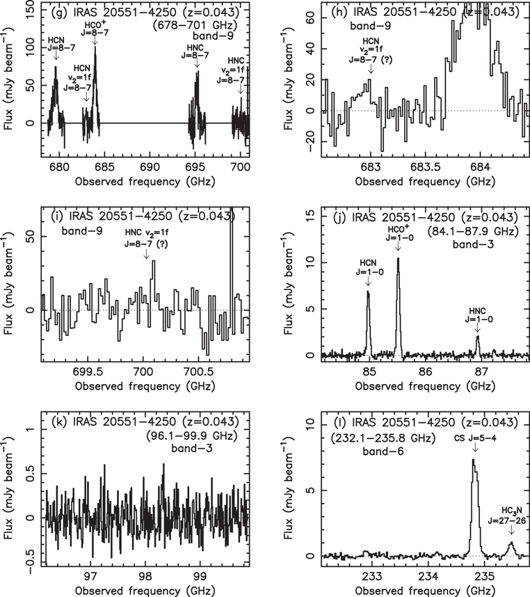
Download figure:
Standard image High-resolution image
Figure 2. Spectra at the continuum peak positions, within the beam size. (a) and (b) are band 7 spectra taken with HCO+ J = 4–3 observations. (c) and (d) are magnified spectra of (a) and (b), respectively, to show serendipitously detected weak emission lines in more detail. In (c), in addition to the primarily targeted major emission lines, downward arrows are shown at the expected redshifted observed frequency with z = 0.043 for some faint molecular lines, SO 8(8)–7(7) ( GHz) and SO2 16(4, 12)–16(3, 13) (
 GHz) + SO 9(8)–8(7) (
 GHz). In (d), down arrows are shown for HOC+ J = 4–3 (
 GHz) and CH3CCH (
 GHz), and up arrows are shown for SO2 6(4, 2)–6(3, 3) (
 GHz) and SO2 20(0, 20)–19(1, 19) (
 GHz). (e) and (f) are band 7 spectra obtained with HNC J = 4–3. In (e), down arrows are shown for CH3OH 4(0, 4)–3(−1, 3) (
 GHz), HNCO 16(5, 11)–15(5, 10) + HNCO 16(5, 12)–15(5, 11) (
 GHz), and H2CO 5(1, 5)–4(1, 4) (
 GHz). In (f), down arrows are shown for SO2 24(1, 23)–24(0, 24) (
 GHz) + SO2 23(2, 22)–23(1, 23) (
 GHz), H2CO 5(3, 3)–4(3, 2) (
 GHz) + H2CO 5(3, 2)–4(3, 1) (
 GHz), and HOCO+ 17(1, 16)–16(1, 15) (
 GHz). (g) is a band 9 spectrum. (h) and (i) are magnified band 9 spectra around HCN v2 = 1f J = 8–7 and HNC v2 = 1f J = 8–7 emission lines, respectively. (j) and (k) are band 3 spectra. (l) and (m) are band 6 spectra. In (l), a down arrow is shown for HC3N J = 27–26 (
 GHz). In (m), down arrows are shown for SO 6(6)–5(5) (
 GHz) and SiO J = 6–5 (
 GHz).
GHz).
Download figure:
Standard image High-resolution imageFor molecular emission lines that are recognizable in the spectra, we created integrated intensity (moment 0) maps, by summing spectral elements displaying discernible signals. These maps are shown in Figure 3 for the primarily targeted main emission lines, and in the Appendix (Figure 17) for serendipitously detected emission lines. All detected molecular lines showed peak positions that agree with those of the simultaneously taken continuum emission, to within 1 pixel (01 for bands 7 and 3, or 003 for bands 9 and 6) in both R.A. and decl. directions. These agreements suggest that the serendipitously detected faint emission lines are likely to be real features, rather than artifacts, with the exceptions of HCO+ v2 = 1f J = 4–3 (band 7), HCN v2 = 1f J = 8–7 (band 9), and HNC v2 = 1f J = 8–7 (band 9), which will be discussed later.

Download figure:
Standard image High-resolution image
Figure 3. Integrated intensity (moment 0) maps of the primarily targeted molecular emission lines in IRAS 20551−4250. The abscissa and ordinate are R.A. (J2000) and decl. (J2000), respectively. Molecular lines observed in ALMA band 7 observations are displayed first (first six images), followed by those in band 9 (five images), band 3 (three images), and band 6 (four images). The contours represent 5σ, 10σ, 20σ, 40σ, and 60σ for CO J = 3–2; 20σ, 40σ, and 60σ for HCO+ J = 4–3; 3σ, 6σ, and 9σ for HCN v2 = 1f J = 4–3; 2σ and 3σ for HCO+ v2 = 1f J = 4–3; 20σ, 40σ, and 60σ for HNC J = 4–3; 4σ, 7σ, and 10σ for HNC v2 = 1f J = 4–3; 3σ and 6σ for HCN J = 8–7; 3σ, 6σ, and 9σ for HCO+ J = 8–7; 3σ and 4.5σ for HNC J = 8–7; 2.5σ and 3σ for HCN v2 = 1f J = 8–7; 10σ, 20σ, and 30σ for HCN J = 1–0; 15σ, 25σ, and 35σ for HCO+ J = 1–0; 3σ, 7σ, and 10σ for HNC J = 1–0; 3σ and 6σ for H13CN J = 3–2, 3σ, and 5σ for H13CO+ J = 3–2; 2.5σ for HN13C J = 3–2; and 15σ and 35σ for CS J = 5–4. For HNC v2 = 1f J = 8–7, no contours with >2σ are seen. The 1σ levels are different for different molecular lines, and are summarized in Table 4. Beam sizes are shown as filled circles in the lower-left region. The displayed areas differ depending on the beam size.
Download figure:
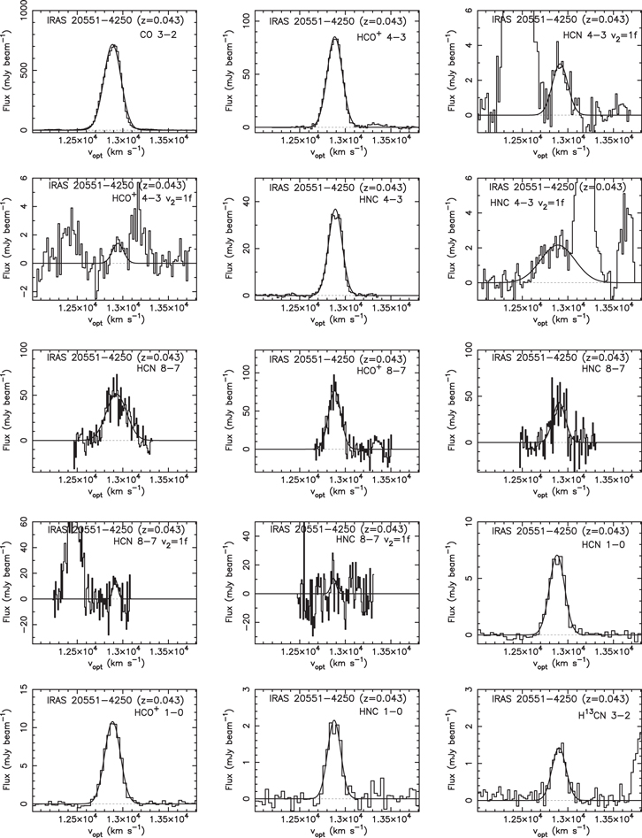
Standard image High-resolution imageFigure 4 shows magnified spectra in the vicinity of the primarily targeted individual molecular emission lines at the continuum peak position within the beam size, together with the best Gaussian fits. The same figures for selected serendipitously detected emission lines are shown in the Appendix (Figure 18). Peak flux values in the moment 0 maps and emission line fluxes estimated from the best Gaussian fits are summarized in Table 4. Table 5 shows the deconvolved, intrinsic emission sizes of the main bright molecular lines and continuum, estimated using the CASA task "imfit."
Download figure:
Standard image High-resolution image
Figure 4. Spectra around individual molecular emission lines. The abscissa is optical LSR velocity ( ≡ c (λ−
 )/
)/ ), and the ordinate is flux in (mJy beam−1). Best Gaussian fits are overplotted with solid curved lines.
Download figure:
Standard image High-resolution imageTable 4. Molecular Line Flux
| Line |

|
Integrated Intensity (Moment 0) Map | Gaussian Line Fit | |||||
|---|---|---|---|---|---|---|---|---|
| (GHz) | Peak | rms | Beam | Velocity | Peak | FWHM | Flux | |
| (Jy beam−1 km s−1) | ('' × '') (°) | (km s−1) | (mJy) | (km s−1) | (Jy km s−1) | |||
| (1) | (2) | (3) | (4) | (5) | (6) | (7) | (8) | (9) |
| CO J = 3–2 | 345.796 | 156.9 (64σ) | 2.46 | 0.83 × 0.65 (−84°) | 12,886 ± 1 | 717 ± 7 | 221 ± 3 | 162 ± 3 |
| HCO+ J = 4–3 | 356.734 | 16.1 (70σ) | 0.23 | 0.85 × 0.67 (74°) | 12,884 ± 1 | 85 ± 1 | 194 ± 2 | 16.9 ± 0.2 |
| HCN J = 4–3 v2 = 1f | 356.256 | 0.49 (9.5σ) | 0.052 | 0.86 × 0.67 (74°) | 12,915 ± 12 | 2.9 ± 0.4 | 200 ± 32 | 0.60 ± 0.13 |
| HCO+ J = 4–3 v2 = 1fa | 358.242 | 0.20 (3.2σ) | 0.062 | 0.81 × 0.66 (84°) | 12,947 ± 34 | 1.4 ± 0.6 | 146 ± 58 | 0.21 ± 0.13 |
| SO 8(8)–7(7)b | 344.311 | 0.55 (9.8σ) | 0.056 | 0.85 × 0.70 (84°) | 12,908 ± 10 | 4.3 ± 0.7 | 148 ± 24 | 0.64 ± 0.15 |
| SO2+SOc | 346.524 + 346.528c | 0.96 (14σ) | 0.068 | 0.83 × 0.65 (−84°) | ⋯ | ⋯ | ⋯ | ⋯ |
| HOC+ J = 4–3d | 357.922 | 0.46 (6.9σ) | 0.067 | 0.86 × 0.69 (82°) | 12,875 ± 21 | 3.0 ± 0.5 | 213 ± 62 | 0.66 ± 0.22 |
| CH3CCH | 358.709–818e | 0.45 (7.0σ) | 0.065 | 0.81 × 0.66 (84°) | 12,900 ± 16 | 2.6 ± 0.5 | 185 ± 39 | 0.49 ± 0.14 |
| HNC J = 4–3 | 362.630 | 6.4 (70σ) | 0.091 | 0.75 × 0.58 (−78°) | 12,890 ± 2 | 37 ± 1 | 177 ± 4 | 6.6 ± 0.2 |
| HNC J = 4–3 v2 = 1ff | 365.147 | 0.64 (11.5σ)f | 0.056f | 0.66 × 0.53 (−83°)f | 12,890 (fix) | 2.2 ± 0.4 | 443 (fix) | 0.98 ± 0.19 |
| H2CO 5(1,5)–4(1,4) | 351.769 | 1.2 (24σ) | 0.051 | 0.63 × 0.52 (−81°) | 12,879 ± 4 | 6.8 ± 0.2 | 213 ± 9 | 1.5 ± 0.1 |
| HOCO+ 17(1,16)–16(1,15)g | 364.804 | 2.5 (42σ) | 0.059 | 0.81 × 0.64 (−83°) | 12,898 ± 2 | 13 ± 1 | 181 ± 4 | 2.5 ± 0.1 |
| HCN J = 8–7 | 708.877 | 12.9 (7.1σ) | 1.8 | 0.24 × 0.21 (88°) | 12,930 ± 9 | 51 ± 3 | 262 ± 19 | 13.7 ± 1.3 |
| HCO+ J = 8–7 | 713.341 | 11.9 (9.9σ) | 1.2 | 0.23 × 0.21 (−88°) | 12,884 ± 4 | 77 ± 4 | 159 ± 10 | 12.5 ± 1.0 |
| HNC J = 8–7 | 725.107 | 6.9 (4.8σ) | 1.4 | 0.23 × 0.20 (90°) | 12,904 ± 10 | 43 ± 5 | 164 ± 21 | 7.2 ± 1.3 |
| HCN J = 8–7 v2 = 1f | 712.372 | 1.0 (3.1σ) | 0.32h | 0.23 × 0.21 (−88°) | 12,918 ± 12 | 15 ± 5 | 61 ± 25 | 1.0 ± 0.5 |
| HNC J = 8–7 v2 = 1f | 730.131 | 0.88 (1.7σ) | 0.52h | 0.23 × 0.20 (88°) | 12,871 ± 30 | 11 (fix) | 67 (fix) | 0.7 |
| HCN J = 1–0 | 88.632 | 1.4 (33σ) | 0.041 | 1.2 × 0.9 (69°) | 12,881 ± 2 | 7.1 ± 0.2 | 195 ± 5 | 1.4 ± 0.1 |
| HCO+ J = 1–0 | 89.189 | 2.2 (40σ) | 0.054 | 1.2 × 0.9 (72°) | 12,888 ± 1 | 11 ± 1 | 202 ± 3 | 2.2 ± 0.1 |
| HNC J = 1–0 | 90.664 | 0.36 (11σ) | 0.034 | 1.0 × 0.7 (61°) | 12,878 ± 5 | 2.2 ± 0.1 | 169 ± 13 | 0.37 ± 0.04 |
| H13CN J = 3–2 | 259.012 | 0.25 (6.8σ) | 0.036 | 0.16 × 0.15 (35°) | 12,903 ± 6 | 1.4 ± 0.1 | 181 ± 16 | 0.26 ± 0.03 |
| H13CO+ J = 3–2 | 260.255 | 0.13 (5.2σ) | 0.024 | 0.16 × 0.16 (59°) | 12,901 ± 8 | 0.86 ± 0.09 | 159 ± 18 | 0.14 ± 0.02 |
| HN13C J = 3–2 | 261.263 | 0.066 (2.8σ) | 0.024 | 0.16 × 0.16 (59°) | 12,911 ± 20 | 0.34 ± 0.07 | 204 ± 51 | 0.071 ± 0.023 |
| CS J = 5–4 | 244.936 | 1.2 (40σ) | 0.030 | 0.19 × 0.17 (38°) | 12,901 ± 2 | 7.5 ± 0.1 | 167 ± 4 | 1.3 ± 0.1 |
| SO 6(6)–5(5) | 258.256 | 0.34 (10σ) | 0.034 | 0.16 × 0.15 (35°) | 12,909 ± 4 | 1.9 ± 0.1 | 187 ± 10 | 0.37 ± 0.03 |
| SiO J = 6–5 | 260.518 | 0.22 (5.8σ) | 0.037 | 0.16 × 0.16 (59°) | 12,902 ± 7 | 1.2 ± 0.1 | 188 ± 15 | 0.24 ± 0.03 |
| HC3N J = 27–26 | 245.606 | 0.15 (6.4σ) | 0.023 | 0.19 × 0.17 (38°) | 12,900 ± 5 | 0.99 ± 0.07 | 154 ± 13 | 0.16 ± 0.02 |
Notes. Column (1): Observed molecular line. Primarily targeted lines are listed first, followed by serendipitously detected lines. Column (2): Rest-frame frequency of each molecular line in (GHz). Column (3): Integrated intensity in (Jy beam−1 km s−1) at the emission peak. Detection significance relative to the rms noise (1σ) in the moment 0 map is shown in parentheses. Possible systematic uncertainty is not included. Column (4): rms noise (1σ) level in the moment 0 map in (Jy beam−1 km s−1), derived from the standard deviation of sky signals in each moment 0 map. Column (5): Synthesized beam in (arcsec × arcsec) and position angle in (°). Position angle is 0° in the north–south direction, and increases in the counter-clockwise direction. Columns (6)–(9): Gaussian fits of emission lines in the spectra at the continuum peak position, within the beam size. Column (6): Optical LSR velocity ( ) of emission peak in (km s−1). Column (7): Peak flux in (mJy). Column (8): Observed FWHM in (km s−1) in Figure 4. Column (9): Flux in (Jy km s−1). The observed FWHM in (km s−1) in column 8 is divided by (
 ) to obtain the intrinsic FWHM in (km s−1).
 GHz) might contaminate.
bHC15N J = 4–3 emission line (
GHz) might contaminate.
bHC15N J = 4–3 emission line ( GHz) might contaminate.
cCombination of SO2 16(4,12)–16(3,13) (
GHz) might contaminate.
cCombination of SO2 16(4,12)–16(3,13) ( GHz) and SO 9(8)–8(7) (
 GHz).
dSO2 6(4,2)–6(3,3) emission line (
GHz).
dSO2 6(4,2)–6(3,3) emission line ( GHz) might contaminate.
eCombination of CH3CCH 21(4)–20(4) (
GHz) might contaminate.
eCombination of CH3CCH 21(4)–20(4) ( GHz), CH3CCH 21(3)–20(3) (
 GHz), CH3CCH 21(2)–20(2) (
 GHz), CH3CCH 21(1)–20(1) (
 GHz), and CH3CCH 21(0)–20(0) (
 GHz).
fAll emission line components with FWHM ∼ 443 km s−1 are integrated.
gH3O+ 3(2)–2(2) emission line (
GHz).
fAll emission line components with FWHM ∼ 443 km s−1 are integrated.
gH3O+ 3(2)–2(2) emission line ( GHz) might contaminate.
hThe rms noise level was determined from the 40–100 pixel annular region around the center of the moment 0 map.
GHz) might contaminate.
hThe rms noise level was determined from the 40–100 pixel annular region around the center of the moment 0 map.
Download table as: ASCIITypeset image
Table 5. Intrinsic Emission Size After Deconvolution for Selected Bright Emission Lines and Continuum
| Line | (mas × mas) (°) | Beam (arcsec × arcsec) |
|---|---|---|
| (1) | (2) | (3) |
| CO J = 3–2 | 828 ± 123, 561 ± 127 (131 ± 23) | 0.83 × 0.65 |
| HCO+ J = 4–3 | 306 ± 35, 275 ± 37 (96 ± 76) | 0.85 × 0.67 |
| cont43a | 348 ± 52, 336 ± 63 (136 ± 88) | 0.84 × 0.68 |
| HNC J = 4–3 | 206 ± 30, 105 ± 55 (152 ± 17) | 0.75 × 0.58 |
| cont43b | 326 ± 26, 284 ± 22 (89 ± 48) | 0.66 × 0.53 |
| HCN J = 8–7 | 218 ± 44, 135 ± 43 (84 ± 38) | 0.24 × 0.21 |
| HCO+ J = 8–7 | 246 ± 36, 179 ± 34 (70 ± 34) | 0.23 × 0.21 |
| HNC J = 8–7 | 141 ± 57, 65 ± 50 (72 ± 74) | 0.23 × 0.20 |
| cont87 | 261 ± 16, 225 ± 15 (56 ± 23) | 0.23 × 0.21 |
| HCN J = 1–0 | 711 ± 138, 655 ± 170 (108 ± 82) | 1.19 × 0.95 |
| HCO+ J = 1–0 | 763 ± 136, 609 ± 221 (142 ± 83) | 1.22 × 0.95 |
| HNC J = 1–0 | 320 ± 222, 45 ± 186 (71 ± 22) | 1.02 × 0.73 |
| cont10 | 510 ± 81, 468 ± 87 (84 ± 87) | 1.09 × 0.87 |
| CS J = 5–4 | 201 ± 13, 152 ± 13 (80 ± 13) | 0.19 × 0.17 |
| cont32 | 198 ± 13, 170 ± 12 (60 ± 28) | 0.18 × 0.17 |
Note. Column (1): Emission line or continuum. Column (2): Intrinsic emission size in mas, after deconvolution using the CASA task "imfit." The position angle in (°) is shown in parentheses. Column (3): Synthesized beam size in arcsec × arcsec, shown for reference.
Download table as: ASCIITypeset image
HCO+ J = 4–3 and HNC J = 4–3 (v = 0) fluxes were obtained in both our ALMA Cycle 0 and 2 observations. Our ALMA Cycle 0 data provided HCO+ J = 4–3 and HNC J = 4–3 (v = 0) fluxes of 14 ± 1 and 5.8 ± 0.2 (Jy km s−1), respectively, based on Gaussian fit, within a 06 × 04 beam size (Imanishi & Nakanishi 2013b). The estimated fluxes based on Gaussian fit in our ALMA Cycle 2 data were 17 ± 1 and 6.6 ± 0.2 (Jy km s−1) for HCO+ J = 4–3 (09 × 07 beam) and HNC J = 4–3 (08 × 06 beam), respectively. The fluxes in ALMA Cycle 2 data were 10%–20% higher than in our ALMA Cycle 0 data. This could be partly due to larger beam sizes in the ALMA Cycle 2 data, if a significant fraction of these emission lines came from a spatially extended region with >05 (>400 pc). However, the nuclear HCO+ J = 4–3 and HNC J = 4–3 emission components were estimated to be spatially compact (Table 5). The 10%–20% flux discrepancy could be largely accounted for by the possible absolute flux calibration uncertainty in individual ALMA Cycle 0 and 2 data (maximum ∼10% for each).
The HCN J = 4–3 (v = 0) line was not covered in our ALMA Cycle 2 observations. In ALMA Cycle 0, the HCN J = 4–3 and HCO+ J = 4–3 lines were simultaneously observed. For the HCO+ J = 4–3 (v = 0) line, our Cycle 2 band 7 data (17 ± 1 Jy km s−1) provided ∼22% higher absolute flux than Cycle 0 (14 ± 1 Jy km s−1). We thus multiplied the HCN J = 4–3 (v = 0) flux derived in our Cycle 0 observations (9.5 ± 0.2 Jy km s−1) (Imanishi & Nakanishi 2013b) by a factor of 1.22, and adopted the re-calibrated HCN J = 4–3 flux with 11.6 ± 0.2 (Jy km s−1) for all subsequent discussion in this paper.
The HCN v2 = 1f J = 4–3 emission line was also observed in both ALMA Cycles 0 and 2. Its detection significance in the moment 0 map (Figure 3) of our Cycle 2 data was >9σ, which is improved from the ∼5σ detection in our Cycle 0 moment 0 map (Imanishi & Nakanishi 2013b), and further confirms the presence of the detectable HCN v2 = 1f J = 4–3 emission line in IRAS 20551−4250. The estimated HCN v2 = 1f J = 4–3 emission line flux, based on Gaussian fit, in the Cycle 0 data was 0.39 ± 0.07 (Jy km s−1), which is converted to 0.47 ± 0.08 (Jy km s−1), after the factor of 1.22 multiplication, because HCN v2 = 1f J = 4–3 and HCO+ J = 4–3 (v = 0) line data were taken simultaneously in our ALMA observations. The flux in the Cycle 2 data is 0.60 ± 0.13 (Jy km s−1). The flux measurements for the Cycle 0 and 2 data are consistent. Given deeper Cycle 2 data than Cycle 0 data, we adopted the HCN v2 = 1f J = 4–3 flux estimated with Gaussian fit in the Cycle 2 data (0.60 ± 0.13 Jy km s−1).
The HNC v2 = 1f J = 4–3 emission line for IRAS 20551−4250 was first covered in our ALMA Cycle 2 observations, and its signature is shown in the band 7 spectrum in Figures 2(f) and 4. Based on the moment 0 map (Figure 3) and Gaussian fit (Table 4), we posit that the HNC v2 = 1f J = 4–3 emission line was detected. However, the line width of the HNC v2 = 1f J = 4–3 emission line (FWHM ∼ 440 km s−1) is substantially larger than other bright molecular emission lines with FWHM ∼ 200 km s−1 (Table 4). Therefore, contamination from other faint molecular emission lines is possible, and the measured HNC v2 = 1f J = 4–3 emission line flux should be taken as an upper limit. If we assume the intrinsic line width of the HNC v2 = 1f J = 3–2 emission line to be FWHM ∼ 200 km s−1, then the actual HNC v2 = 1f J = 3–2 emission line flux will be about half of that shown in Table 4.
For the HCO+ v2 = 1f J = 4–3 emission line, we barely see the 3.2σ peak at the nuclear position in the moment 0 map (Figure 3). However, the contour size at the peak is significantly smaller than the synthesized beam size, and emissions with similar 3σ level contours were seen at some other off-nuclear regions (Figure 3), making the existence of this 3.2σ peak uncertain. In Figure 2(d), an emission-like feature may be present close to the expected frequency of the HCO+ v2 = 1f J = 4–3 line; however, its observed peak seems to be slightly offset from the expected frequency at z = 0.043 (shown as a downward arrow). Based on Gaussian fit, the peak velocity of this emission-like feature ( km s−1) was significantly higher than other bright molecular emission lines detected in band 7 (
 km s−1), and the detection significance is <2σ (Table 4). Detection of the HCO+ v2 = 1f J = 4–3 emission line has never been reported in any external galaxy. We require higher signal-to-noise ratio (S/N) data to improve the constraining of the strength of this yet-to-be-detected HCO+ v2 = 1f J = 4–3 emission line.
The HCN v2 = 1f J = 8–7 ( GHz) and HNC v2 = 1f J = 8–7 (
 GHz) lines were covered in our ALMA band 9 spectrum, while the HCO+ v2 = 1f J = 8–7 (
 GHz) line was not. In Figures 2(h) and (i), subtle signatures of emission lines are observed close to the expected frequencies of redshifted HCN v2 = 1f J = 8–7 and HNC v2 = 1f J = 8–7 lines, respectively. However, their detection significance, based on Gaussian fit, is <3σ. In the moment 0 map of HCN v2 = 1f J = 8–7, we see a 3.1σ emission peak at the nuclear position, but the 3σ contour was much smaller than the synthesized beam size (Figure 3). Detection of v2 = 1f J = 8–7 lines of HCN and HNC was unclear, and we will need data with higher S/N to quantitatively discuss their fluxes.
The H13CN J = 3–2 emission lines were observed in ALMA Cycle 2 (36 minutes integration) and Cycle 4 (129 minutes integration). The flux measurements, based on Gaussian fit, were 0.37 ± 0.05 (Jy km s−1) with 053 × 047 (Imanishi et al. 2016b) and 0.26 ± 0.03 (Jy km s−1) with 016 × 015 in Cycles 2 and 4, respectively. The smaller flux measurement in Cycle 4 could be largely explained by the smaller beam size and maximum 10% absolute flux calibration uncertainty in individual ALMA observations. We adopted our Cycle 4 measurement for the following two reasons: (1) The primary aim of our isotopologue observations is to estimate the flux attenuation by line opacity for HCN, HCO+, and HNC J = 3–2 emission. (2) Our Cycle 4 data contain H13CN, H13CO+, and HN13C J = 3–2 emission line flux measurements with similar beam sizes. Adopting our Cycle 4 measurement of the H13CN J = 3–2 flux is a more straightforward way to compare and correct flux attenuation for the HCN, HCO+, and HNC J = 3–2 emission lines.
Figure 5 presents intensity-weighted mean velocity (moment 1) and intensity-weighted velocity dispersion (moment 2) maps of selected bright emission lines in band 7, CO J = 3–2, HCO+ J = 4–3, and HNC J = 4–3. The CO J = 3–2 emission line was detected not only in the nuclear region, but also in spatially extended outer regions. In addition to the much higher flux of CO J = 3–2 than other molecular lines, its lower critical density is likely to contribute to the detection of the spatially extended structure because outer low-density molecular gas can collisionally excite CO J = 3–2 more than HCO+ J = 4–3 and HNC J = 4–3. Figure 6 shows moment 1 and 2 maps of HCN, HCO+, and HNC J = 8–7 emission lines in band 9 for the central zoomed regions. Velocity information is available only for the nuclear compact regions. The moment 1 and 2 maps for HCN, HCO+, and HNC J = 1–0 emission lines in band 3 are presented in Figure 7, where we can obtain velocity information for spatially extended regions outside the synthesized beam sizes—at least for HCN and HCO+. In Figure 8, the moment 1 and 2 maps of the CS J = 5–4 emission line in band 6, the additional dense molecular gas tracer (Greve et al. 2014), are presented. Overall, most of the bright emission lines of dense molecular gas tracers display similar rotational patterns, showing that the northeastern region of the nucleus is more redshifted than the southwestern region.

Figure 5. (Top) Intensity-weighted mean velocity (moment 1) maps for the CO J = 3–2, HCO+ J = 4–3, and HNC J = 4–3 emission lines in band 7. The abscissa and ordinate are R.A. (J2000) and decl. (J2000), respectively. The contours represent 12,850, 12,900, and 12,950 km s−1 for CO J = 3–2; 12,870, 12,895, and 12,920 km s−1 for HCO+ J = 4–3; and 12,875, 12,890, and 12,905 km s−1 for HNC J = 4–3. (Bottom) Intensity-weighted velocity dispersion (moment 2) maps. The contours represent 40, 60, and 80 km s−1 for CO J = 3–2; 40 and 60 km s−1 for HCO+ J = 4–3; and 50 and 60 km s−1 for HNC J = 4–3. The centers of the CO J = 3–2 images are slightly displaced from those of the HCO+ J = 4–3 and HNC J = 4–3 images, to show the whole extended structures. Beam sizes are shown as open circles at the lower-left. We applied an appropriate cut-off to prevent the resulting maps from being dominated by noise. In the left two panels, the continuum peak positions are marked with crosses.
Download figure:
Standard image High-resolution image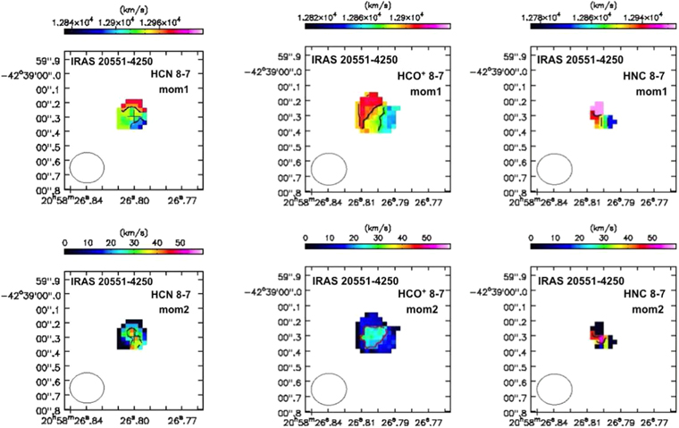
Figure 6. (Top) Intensity-weighted mean velocity (moment 1) maps for HCN J = 8–7, HCO+ J = 8–7, and HNC J = 8–7 emission lines in band 9. The abscissa and ordinate are R.A. (J2000) and decl. (J2000), respectively. The contours represent 12,900 and 12,950 km s−1 for HCN J = 8–7; 12,875 and 12,900 km s−1 for HCO+ J = 8–7; and 12,850 and 12,900 km s−1 for HNC J = 8–7. (Bottom) Intensity-weighted velocity dispersion (moment 2) maps. The contours represent 30 km s−1 for HCN J = 8–7, 20 km s−1 for HCO+ J = 8–7, and 40 km s−1 for HNC J = 8–7. Only smaller central areas are displayed, because the beam size achieved in band 9 was much smaller than those of bands 7 and 3. Beam sizes are shown as open circles at the lower-left part. An appropriate cut-off was chosen for these moment 1 and 2 maps. In the left panels, the continuum peak positions are marked with crosses.
Download figure:
Standard image High-resolution image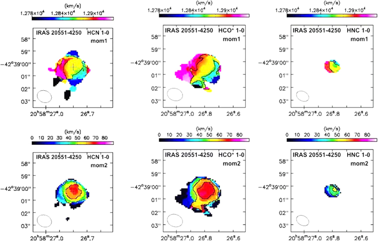
Figure 7. (Top) Intensity-weighted mean velocity (moment 1) maps for HCN J = 1–0, HCO+ J = 1–0, and HNC J = 1–0 emission lines in band 3. The abscissa and ordinate are R.A. (J2000) and decl. (J2000), respectively. The contours represent 12,860 and 12,900 km s−1 for HCN J = 1–0; 12,860 and 12,900 km s−1 for HCO+ J = 1–0; and 12,860 and 12,890 km s−1 for HNC J = 1–0. (Bottom) Intensity-weighted velocity dispersion (moment 2) maps. The contours represent 40 and 60 km s−1 for HCN J = 1–0; 53 and 66 km s−1 for HCO+ J = 1–0; and 40 and 50 km s−1 for HNC J = 1–0. Beam sizes are shown as open circles in the lower-left region. An appropriate cut-off was chosen for these moment 1 and 2 maps. In the left panels, the continuum peak positions are marked with crosses.
Download figure:
Standard image High-resolution image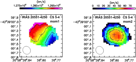
Figure 8. (Left) Intensity-weighted mean velocity (moment 1) map for CS J = 5–4 in band 6. The abscissa and ordinate are R.A. (J2000) and decl. (J2000), respectively. The contours represent 12,850, 12,900, and 12,950 km s−1. (Right) Intensity-weighted velocity dispersion (moment 2) map. The contours represent 35 and 50 km s−1. The image size is the same as that of band 9 data in Figure 6. Beam sizes are shown as open circles in the lower-left region. An appropriate cut-off was chosen for these moment 1 and 2 maps. The continuum peak positions are marked with crosses.
Download figure:
Standard image High-resolution imageTable 6 provides the luminosities of the primarily targeted molecular emission lines. In addition to the HCN, HCO+, and HNC emission lines at various rotational J-transitions at v = 0 and v2 = 1f, the isotopologue H13CN, H13CO+, HN13C J = 3–2, CO J = 3–2, and CS J = 5–4 emission lines at v = 0 are tabulated.
Table 6. Luminosity of Selected Molecular Emission Lines
| Line | Flux (Jy km s−1) | 104 ( ) ) |
107 (K km s−1 pc2) |
|---|---|---|---|
| HCN J = 1–0 | 1.4 ± 0.1 | 0.44 ± 0.03 | 19.6 ± 1.4 |
| HCN J = 3–2 | 5.9 ± 0.1a | 5.5 ± 0.1a | 9.2 ± 0.2a |
| HCN J = 4–3 | 11.6 ± 0.2b | 14.5 ± 0.3b | 10.1 ± 0.2b |
| HCN J = 8–7 | 13.7 ± 1.3 | 34.1 ± 3.2 | 3.0 ± 0.3 |
| HCN v2 = 1f J = 3–2 | 0.25 ± 0.07a | 0.23 ± 0.07a | 0.35 ± 0.10a |
| HCN v2 = 1f J = 4–3 | 0.60 ± 0.13 | 0.75 ± 0.16 | 0.52 ± 0.11 |
| HCO+ J = 1–0 | 2.2 ± 0.1 | 0.69 ± 0.03 | 30.4 ± 1.4 |
| HCO+ J = 3–2 | 8.4 ± 0.1a | 7.9 ± 0.1a | 12.9 ± 0.2a |
| HCO+ J = 4–3 | 16.9 ± 0.2 | 21.2 ± 0.3 | 14.6 ± 0.2 |
| HCO+ J = 8–7 | 12.5 ± 1.0 | 31.3 ± 2.5 | 2.7 ± 0.2 |
| HCO+ v2 = 1f J = 3–2 | <0.088a | <0.084a | <0.13a |
| HCO+ v2 = 1f J = 4–3 | <0.20 | <0.26 | <0.18 |
| HNC J = 1–0 | 0.37 ± 0.04 | 0.12 ± 0.01 | 4.9 ± 0.5 |
| HNC J = 3–2 | 3.2 ± 0.1a | 3.1 ± 0.1a | 4.7 ± 0.1a |
| HNC J = 4–3 | 6.6 ± 0.2 | 8.4 ± 0.3 | 5.5 ± 0.2 |
| HNC J = 8–7 | 7.2 ± 1.3 | 18.3 ± 3.3 | 1.5 ± 0.3 |
| HNC v2 = 1f J = 3–2 | 0.20 ± 0.07a | 0.19 ± 0.07a | 0.27 ± 0.09a |
| HNC v2 = 1f J = 4–3 | 0.98 ± 0.19 | 1.3 ± 0.2 | 0.81 ± 0.16 |
| H13CN J = 3–2 | 0.26 ± 0.03 | 0.24 ± 0.03 | 0.43 ± 0.05 |
| H13CO+ J = 3–2 | 0.14 ± 0.02 | 0.13 ± 0.02 | 0.23 ± 0.03 |
| HN13C J = 3–2 | 0.071 ± 0.023 | 0.065 ± 0.021 | 0.11 ± 0.04 |
| CO J = 3–2 | 162 ± 3 | 197 ± 4 | 149 ± 3 |
| CS J = 5–4 | 1.3 ± 0.1 | 1.1 ± 0.1 | 2.4 ± 0.2 |
Column (1): Emission line. Column (2): Adopted values for the observed flux in (Jy km s−1) shown for reference. Column (3): Luminosity in units of ( ), calculated with Equation (1) of Solomon & Vanden Bout (2005). Column (4): Luminosity in units of (K km s−1 pc2), calculated with Equation (3) of Solomon & Vanden Bout (2005).
Notes.
aTaken from Imanishi et al. (2016b). bOriginally taken from ALMA Cycle 0 data by Imanishi & Nakanishi (2013b) and multiplied by a factor of 1.22 to correct for the flux difference between Cycle 0 and 2 data. See Section 3 for more detail.Download table as: ASCIITypeset image
4. Discussion
4.1. Molecular Gas Morphology and Dynamics
Continuum and molecular line emission are dominated by a nuclear compact component; however, in the brightest CO J = 3–2 integrated-intensity (moment 0) map in Figure 3, a spatially extended structure is seen southeast of the nucleus. A similar extended structure is seen in the stellar emission probed in the near-infrared K-band (2.2 μm) image (Duc et al. 1997), suggesting that this extended CO J = 3–2 emission originates in the host galaxy.
In the intensity-weighted mean velocity (moment 1) maps of CO J = 3–2, J = 1–0, 3–2, 4–3, and 8–7 of HCN, HCO+, HNC, and CS J = 5–4 in Figures 5–8 and Imanishi et al. (2016b), as well as CO J = 1–0 in Ueda et al. (2014), the overall dynamics are dominated by rotational motion in such a way that the northeastern part is redshifted and the southwestern part is blueshifted, relative to the nucleus. However, in the moment 1 map of the brightest CO J = 3–2 emission line, a dynamically decoupled component from the overall rotation is seen at the southwesternmost region (the clump at the lower-right edge in Figure 5). A plausible explanation is that some type of merger event happened previously, which is quite reasonable given that IRAS 20551−4250 is a ULIRG and ULIRGs are usually driven by gas-rich galaxy mergers (Sanders & Mirabel 1996).
In Figure 4, although we fit emission lines with single Gaussian component, when we examine the line profiles of the very bright CO J = 3–2 and HCO+ J = 4–3 emission lines in more detail, skew patterns are recognizable. To investigate the skewed asymmetric line profiles in more detail, we fit these bright emission lines with a Gaussian component, only using data points at the red part of the emission peak (Figures 9(a) and (b)) and at the blue part of the emission peak (Figures 9(c) and (d)). When we fit the red component, the data in the blue part indicates an excess, compared to the best Gaussian fit. Conversely, when we fit with a Gaussian, using data at the blue part of the emission peak only, the extrapolation of the best-fit Gaussian to the redder part is higher than the actual data, particularly for CO J = 3–2. The full-width at half maximum (FWHM) values of the best fit Gaussian are 260 km s−1 and 165 km s−1 for the blue and red components of the CO J = 3–2 emission line, respectively. These are 205 km s−1 and 160 km s−1 for the blue and red components of the HCO+ J = 4–3 emission line, respectively. We thus quantitatively confirm that the line widths are larger for the blue components than the red components both for CO J = 3–2 and HCO+ J = 4–3. Figure 10 displays the contours of the blue and red components of the CO J = 3–2 and HCO+ J = 4–3 emission lines. The red component is slightly offset to the northeastern direction from the blue component; this could be explained by the overall rotational motion of IRAS 20551−4250. A natural interpretation for this skewed profile is that turbulence is stronger at the blueshifted molecular gas-emitting region, which broadens the line width at the blue side. In the CO J = 3–2 moment 1 map in Figure 5, the signature of a merger-induced distinct emission component is seen at the blueshifted southwestern part of the nucleus. This possible merger-induced turbulence component may contribute to the observed broader emission line profile for the blue component.

Figure 9. (a) Gaussian fit only for the redder part of the emission peak for CO J = 3–2 ( > 12,905 km s−1). (b) The same fit as (a), for HCO+ J = 4–3 (
 > 12,905 km s−1). (c) Gaussian fit only for the bluer part of the emission peak for CO J = 3–2 (
 < 12,905 km s−1). (d) The same fit as (c), for HCO+ J = 4–3 (
 < 12,905 km s−1).
Download figure:
Standard image High-resolution image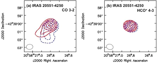
Figure 10. (a) Contours of the blue ( km s−1) and red (
 km s−1) components of the CO J = 3–2 emission line. The blue and red components are shown as blue dashed and red solid contours, respectively. The contours represent 5σ, 10σ, 20σ, 40σ, and 60σ for both blue and red components. The 1σ level is 1.3 (Jy beam−1 km s−1) for the blue component and 1.0 (Jy beam−1 km s−1) for the red component. (b) Contours of the blue (
 km s−1; blue dashed lines) and red (
 km s−1; red solid lines) components of the HCO+ J = 4–3 emission line. The contours represent 5σ, 10σ, 20σ, 40σ, and 60σ (1σ is 0.12 and 0.10 [Jy beam−1 km s−1] for the blue and red components, respectively).
Download figure:
Standard image High-resolution imageIn Figure 11(a), we show a zoom-in of the bottom part of the very bright CO J = 3–2 emission line, with the best Gaussian fit of this line (Figure 4 and Table 4) overplotted. There are clear excesses at both the blue and red sides of the CO J = 3–2 emission line, although at the red side, possible contamination from the H13CN J = 4–3 ( GHz) emission line makes quantitative discussion of the broad CO J = 3–2 emission component difficult. This kind of profile is typically interpreted to be due to the broad emission component by outflow activity (Feruglio et al. 2010; Alatalo et al. 2011; Aalto et al. 2012; Maiolino et al. 2012; Cicone et al. 2014; Garcia-Burillo et al. 2015). Figure 11(b) displays the contours of the emission at the blue and red parts of the broad emission component defined in Figure 11(a). The peak position of the red broad component is slightly shifted to the southeast, compared to that of the blue broad component (1 pix left and 1 pix lower with the pixel scale of 01 pix−1). Considering the peak positional accuracy of the blue and red broad components with (beam-size)/(S/N), the significance of this positional displacement is marginal. However, this pattern is different from the global rotation of IRAS 20551−4250. We may be witnessing CO J = 3–2 outflow toward (away from) us being ejected in the northwestern (southeastern) direction from the nucleus.
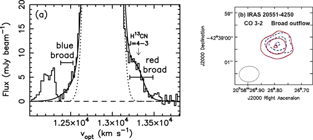
Figure 11. (a) Magnified spectrum at the bottom part of the CO J = 3–2 emission line and its best single Gaussian fit (using all CO J = 3–2 emission line) (the dotted curved line), to show the presence of a broad emission line component. The expected frequency of the H13CN J = 4–3 line is indicated as a downward arrow. The solid horizontal straight lines, inserted by two short vertical lines, indicate the velocity range to create moment 0 maps of the blue and red broad emission components. The velocity ranges are  = 12,382–12,528 km s−1 and 13,209–13,486 km s−1 for the blue and red broad components, respectively. For the thick, solid, curved line, a Gaussian with FWHM = 540 km s−1 and velocity peak at 12886 km s−1 represents the putative outflow-origin broad emission component, and another Gaussian with FWHM = 190 km s−1 takes into account the H13CN J = 4–3 emission line. They are added to the single Gaussian component, shown as a dotted curved line. (b) Contour maps of the blue (blue dashed line) and red (red solid line) broad emission components, defined in Figure 11(a). The contours represent 3σ, 5σ, and 7σ (1σ is 0.055 Jy beam−1 km s−1) for the blue broad component, and 4σ, 8σ, and 12σ (1σ is 0.10 Jy beam−1 km s−1) for the red broad component. For the red broad component, contamination from H13CN J = 4–3 emission line is likely to be present.
Download figure:
Standard image High-resolution imageIn Figure 11(a), we added a Gaussian with FWHM = 540 km s−1 and velocity peak at 12,886 km s−1 for the broad outflow component, and another Gaussian with FWHM = 190 km s−1 to incorporate the H13CN J = 4–3 emission line at the red part of the bright CO J = 3–2 emission line. The Gaussian fit fluxes of the broad CO J = 3–2 emission line component and the H13CN J = 4–3 emission line at the tail of the very bright CO J = 3–2 emission line are estimated to be ∼7.7 (Jy km s−1) and ∼0.9 (Jy km s−1), respectively.
We here estimate a molecular outflow rate from our CO J = 3–2 emission line data. The peak flux value of the blue broad emission component in Figure 11(b) is ∼0.4 (Jy km s−1). We adopt the value of the blue broad component because the red broad component is likely to be contaminated by the H13CN J = 4–3 emission line. Assuming that the outflow-origin red broad component is comparable to the blue broad component, we obtain ∼0.8 (Jy km s−1) for outflow-origin CO J = 3–2 emission. This is a factor of ∼10 smaller than the Gaussian fit flux of the broad CO J = 3–2 emission line component, but we adopt the value of ∼0.8 (Jy km s−1) to obtain the conservative estimate of a molecular outflow rate. We obtain the CO J = 3–2 luminosity with  (K km s−1 pc2) (Solomon & Vanden Bout 2005). Assuming that CO J = 3–2 emission is optically thick and thermalized, and adopting the ULIRG-like CO luminosity to molecular mass (
 ) conversion factor with
  (K km s−1 pc2)−1 (Cicone et al. 2014), we obtain a molecular outflow mass of
  . In Figure 11(b), the peak position difference between the blue broad and red broad emission component is ∼014 or ∼120 (pc). Adopting the outflow peak position offset with R ∼ 60 (pc) from the nucleus and outflow velocity with V = 500 km s−1 (in Figure 11(a), the broad wing component extends to approximately ± 500 km s−1 with respect to the systemic velocity of
  km s−1), we obtain a molecular outflow rate with
  (
( yr−1), where we adopt the relation of
  (Maiolino et al. 2012; Cicone et al. 2014). Assuming ∼30% AGN contribution to the infrared luminosity of IRAS 20551−4250 (i.e.,
  erg s−1), the derived molecular outflow rate with
  (
( yr−1) agrees within a factor of ∼2 with the relation seen in other ULIRGs (Cicone et al. 2014). The molecular outflow kinetic power is estimated to be
  (erg s−1), which is ∼1% of the AGN luminosity. The molecular outflow momentum rate is
  × V ∼ 4.6 × 1030 (kg m s−2), which is ∼12 × LAGN/c. These values are comparable to those observed in other ULIRGs with detectable molecular outflow activity (Cicone et al. 2014). Note that all of molecular outflow mass (
 ), molecular outflow rate (
 ), molecular outflow kinetic power (
 ), and molecular outflow momentum rate (
 ) could increase by an order of magnitude, if we use the Gaussian fit flux of the broad CO J = 3–2 emission line component.
4.2. Isotopologue Molecular Lines and Opacity Estimate
From Table 4 and Imanishi et al. (2016b), we obtained the ratios of HCN-to-H13CN J = 3–2 flux in (Jy km s−1) to be ∼22 ± 3, HCO+-to-H13CO+ J = 3–2 flux in (Jy km s−1) to be ∼60 ± 9, and HNC-to-HN13C J = 3–2 flux in (Jy km s−1) to be ∼45 ± 15. We must note that the detection significance of HN13C J = 3–2 is only ∼3σ in both Gaussian fit in the spectrum and moment 0 map. Thus, discussion of HNC could be more uncertain than HCN and HCO+. Adopting the 12C-to-13C abundance ratios in ULIRGs with 50–100 (Henkel & Mauersberger 1993; Henkel et al. 1993; Martin et al. 2010; Henkel et al. 2014), we find that the flux attenuation by line opacity for HCN J = 3–2 is estimated to be a factor of 2–5, while those of HCO+ J = 3–2 and HNC J = 3–2 are a factor of ∼1–1.5 and ∼1–2, respectively, where we assume that isotopologue emission lines are optically thin (Jimenez-Donaire et al. 2017).
In a geometry where radiation sources and molecular gas are spatially well mixed, the flux attenuation and optical depth (τ) are related as  . From this relationship, we obtain τ = 2–5 for HCN J = 3–2. Using the estimated H13CN J = 4–3 flux with ∼0.9 (Jy km s−1) (Section 4.1), we obtain the ratio of HCN-to-H13CN J = 4–3 flux in (Jy km s−1) to be ∼13. The flux attenuation by line opacity for HCN J = 4–3 is estimated to be 4–7 or τ = 4–7, which is comparable to that for HCN J = 3–2 (τ = 2–5). In summary, our isotopologue observations suggest that the HCN J = 3–2 and J = 4–3 emission lines are considerably flux-attenuated by line opacity.
In contrast, the relatively small flux attenuation with <2 suggests that the line opacity for HCO+ J = 3–2 and HNC J = 3–2 is τ < 1.5. Based on the observed HCN, HCO+, and HNC J = 3–2 fluxes at v2 = 1f and v = 0, and calculation of vibrational excitation by infrared radiative pumping, using the available 5–30 μm spectrum of IRAS 20551−4250, Imanishi et al. (2016b) argued that HCN abundance is higher than those of HCO+ and HNC. This higher HCN abundance scenario is a plausible explanation for the higher HCN line opacity than HCO+ and HNC at J = 3–2.
4.3. Infrared Radiative Pumping and Independent Molecular Abundance Estimate
Based on the fluxes of vibrationally excited (v2 = 1f) and vibrational ground (v = 0) HCN, HCO+, and HNC emission lines at J = 3–2, it has been estimated that the infrared radiative pumping mechanism plays a role in rotational excitation at v = 0 in IRAS 20551−4250, at least for HCN and HNC (Imanishi et al. 2016b). Namely, once HCN and HNC are vibrationally excited to v2 = 1 by absorbing infrared ∼14 μm and ∼22 μm photons, respectively, they are decayed back to v = 0 and their rotational J-transition fluxes at v = 0 can be higher than those for collisional excitation alone (Rangwala et al. 2011). We here attempt to confirm this result, based on our newly collected ALMA data. The J = 1–0 line is not present at the vibrationally excited level (v2 = 1). For J = 8–7, v2 = 1f emission lines are not clearly detected, mainly due to large background noise at this high ALMA frequency range. We thus focus on J = 4–3 data, and follow the same logical steps as those made by Imanishi et al. (2016b) for J = 3–2 data.
Infrared radiative pumping is estimated to play a significant role if the following condition is met:
where  is the v2 = 1f vibrational excitation temperature, T0 is the energy level at v2 = 1f J = 4,
  is the Einstein A coefficient from v2 = 1f to v = 0, and
  is the Einstein A coefficient from J = 4 to J = 3 at v = 0 (Carrol & Goldsmith 1981; Sakamoto et al. 2010; Mills et al. 2013).
Adopting the values in Table 7, and  = ∼1.7 s−1, ∼3.0 s−1, and ∼5.2 s−1 for HCN, HCO+, and HNC, respectively (Deguchi et al. 1986; Aalto et al. 2007; Mauclaire et al. 1995), we obtain ∼160 (K), ∼185 (K), and ∼210 (K) in the right-hand column of Equation (1) for HCN, HCO+, and HNC, respectively. The observed
  values in the left-hand column of Equation (1)—derived based on, e.g., Equation (2) of Imanishi et al. (2016b)—are ∼360 (K), <280 (K), and ∼360 (K) for HCN, HCO+, and HNC, respectively (Table 8). For HCN and HNC, the condition is fulfilled. If the HNC v2 = 1f J = 4–3 flux is approximately half that shown in Table 4 (Section 3), the left-hand column of Equation (1) for HNC is ∼260 (K), which is still higher than the right-hand column. For HCO+, the upper limit of
  still allows the condition to be met.
Table 7. Parameters for Molecular Transition Lines
| Line | Frequency |

|

|
Flux |
|---|---|---|---|---|
| (GHz) | (K) | (10−3 s−1) | (Jy km s−1) | |
| (1) | (2) | (3) | (4) | (5) |
| HCN J = 1–0 | 88.632 | 4.3 | 0.024 | 1.4 ± 0.1 |
| HCN J = 3–2 | 265.886 | 25.5 | 0.84 | 5.9 ± 0.1 |
| HCN J = 4–3 | 354.505 | 42.5 | 2.1 | 11.6 ± 0.2 |
| HCN J = 8–7 | 708.877 | 153.1 | 17.4 | 13.7 ± 1.3 |
| HCN J = 3–2, v2 = 1f | 267.199 | 1050.0 | 0.73 | 0.25 ± 0.07 |
| HCN J = 4–3, v2 = 1f | 356.256 | 1067.1 | 1.9 | 0.60 ± 0.13 |
| HCO+ J = 1–0 | 89.189 | 4.3 | 0.042 | 2.2 ± 0.1 |
| HCO+ J = 3–2 | 267.558 | 25.7 | 1.5 | 8.4 ± 0.1 |
| HCO+ J = 4–3 | 356.734 | 42.8 | 3.6 | 16.9 ± 0.2 |
| HCO+ J = 8–7 | 713.341 | 154.1 | 30.2 | 12.5 ± 1.0 |
| HCO+ J = 3–2, v2 = 1f | 268.689 | 1217.4 | 1.3 | <0.088 |
| HCO+ J = 4–3, v2 = 1f | 358.242 | 1234.6 | 3.4 | <0.20 |
| HNC J = 1–0 | 90.664 | 4.4 | 0.027 | 0.37 ± 0.04 |
| HNC J = 3–2 | 271.981 | 26.1 | 0.93 | 3.2 ± 0.1 |
| HNC J = 4–3 | 362.630 | 43.5 | 2.3 | 6.6 ± 0.2 |
| HNC J = 8–7 | 725.107 | 156.6 | 19.4 | 7.2 ± 1.3 |
| HNC J = 3–2, v2 = 1f | 273.870 | 692.0 | 0.85 | 0.20 ± 0.07 |
| HNC J = 4–3, v2 = 1f | 365.147 | 709.6 | 2.2 | 0.98 ± 0.19 |
Note. Column (1): Molecular transition line. Column (2): Rest-frame frequency in (GHz). Column (3): Upper energy level in (K). Column (4): Einstein A coefficient for spontaneous emission in (10−3 s−1). Values in Columns (3) and (4) are from the Cologne Database of Molecular Spectroscopy (CDMS) (Müller et al. 2005) via Splatalogue (http://www.splatalogue.net). Column (5): Flux in (Jy km s−1) estimated based on Gaussian fit (Table 4, column 9 of this paper; Imanishi & Nakanishi 2013b; Imanishi et al. 2016b). For the undetected HCO+ v2 = 1f J = 3–2 and J = 4–3 emission lines, upper limits based on the integrated intensity (moment 0) maps are adopted.
Download table as: ASCIITypeset image
Table 8. Excitation Temperature for IRAS 20551−4250
| Molecule | (v2,J; v, J) |
 (K) (K) |
|---|---|---|
| (1) | (2) | (3) |
| HCN | (1f, 4; 0, 4) | 360 |
| HCO+ | (1f, 4; 0, 4) | <280 |
| HNC | (1f, 4; 0, 4) | 360 |
| HCN | (0, 3; 0, 1) | 7 |
| (0, 4; 0, 3) | 36 | |
| (0, 8; 0, 4) | 42 | |
| HCO+ | (0, 3; 0, 1) | 7 |
| (0, 4; 0, 3) | 38 | |
| (0, 8; 0, 4) | 36 | |
| HNC | (0, 3; 0, 1) | 10 |
| (0, 4; 0, 3) | 41 | |
| (0, 8; 0, 4) | 42 | |
Notes. Column (1): Molecule. Column (2): Transition. Column (3): Excitation temperature ( ) in (K), derived from observed fluxes. Different beam sizes among different J-transition lines are not considered, in order to be consistent with our previous estimates (Imanishi et al. 2016b).
Download table as: ASCIITypeset image
The left-hand column of Equation (1) will decrease if flux attenuation by line opacity is significant for some v = 0 lines and the intrinsic line opacity-corrected flux at v = 0 and v2 = 1f is used for the calculation. From our isotopologue observations, we see that HCN J = 4–3 flux is estimated to be attenuated by line opacity with a factor of 4–7. Adopting a factor of 5 flux attenuation for HCN J = 4–3, the  value of HCN decreases only to ∼230 (K). Equation (1) is still fulfilled for HCN, not changing the above conclusion. For HCO+ and HNC, flux attenuation by line opacity is not significant at J = 3–2 (Imanishi et al. 2016b). Assuming that this is also the case for J = 4–3, the condition in Equation (1) is still valid for HNC J = 4–3. Thus, it is confirmed from our new ALMA J = 4–3 data that the role of infrared radiative pumping is significant in IRAS 20551−4250, at least for HCN and HNC.
As discussed in Imanishi et al. (2016b), if the column density at v = 0 is the same for HCN, HCO+, and HNC, and if all molecular lines are emitted from the same regions, the ratio of the infrared radiative pumping rate among HCN, HCO+, and HNC in IRAS 20551−4250 is calculated to be

and the v2 = 1 to v = 0 column density ratio among HCN, HCO+, and HNC is calculated to be
based on the Einstein A coefficients of HCN, HCO+, and HNC in Table 7, and the infrared 5–35 μm spectrum of IRAS 20551−4250 obtained with Spitzer IRS (Imanishi et al. 2016b). In essence, the number of infrared photons at ∼22 μm (corresponding to the vibrational-rotational transitions for HNC) is higher than at 12–14 μm (corresponding to the vibrational-rotational transitions of HCN and HCO+), such that it is naively expected that HNC is more vibrationally excited by infrared radiative pumping than HCN and HCO+.
The ratio of the column density at the v2 = 1f J = 4 level ( ) among HCN, HCO+, and HNC is derived with ∝
 , where the line flux from the upper (u) to lower (l) transition level is in units of (Jy km s−1) and Aul is the Einstein A coefficient for spontaneous emission from the upper (u) to lower (l) level (Goldsmith & Langer 1999; Izumi et al. 2013; Imanishi et al. 2016b). From observational fluxes in Table 4 and Einstein A coefficients in Table 7, we obtain the column density ratio at J = 4 at v2 = 1

where we adopt that the actual flux of HNC v2 = 1f J = 3–2 emission line is half of the Gaussian fitted result from Table 4 (see Section 3).
Assuming that the fraction of J = 4 level, relative to all J-levels at v = 0, does not differ significantly among HCN, HCO+, and HNC,5 and that v2 = 1f J-transition emission is optically thin (Imanishi et al. 2016b), Equations (3) (prediction) and (4) (observation) can be reconciled if the column density at v = 0 (Nv = 0) (and thereby abundance) for HCN is higher than HCO+ and HNC by factors of >2.5 and ∼10, respectively. Thus, we obtain an abundance ratio of

The HCN-to-HCO+ abundance ratio of >2.5 and HCN-to-HNC abundance ratio of ∼10 are comparable to those derived from J = 3–2 data (Imanishi et al. 2016b). The HCN-to-HNC abundance ratios derived in this manner at J = 4–3 and J = 3–2 (∼10) appear to be larger than that from isotopologue observations (∼2). This discrepancy could be partly explained by the possibly large ambiguity of the HN13C J = 3–2 flux, which is due to its marginal (∼3σ) detection (Section 4.2). Although a quantitatively accurate estimate of the actual HCN-to-HNC abundance ratio is subject to further investigation, two independent methods consistently suggest that HCN abundance is higher than HCO+ and HNC, by at least a few times.
4.4. Molecular Gas Properties
To obtain a better understanding of the physical properties of these line-emitting molecular gases, we use the RADEX software (van der Tak et al. 2007), which treats the non-LTE analysis and predicts molecular line flux ratios at v = 0 by solving the excitation of rotational transitions at v = 0 by collision, based on the large velocity gradient (LVG) approximation. Free parameters are the number density of hydrogen molecule ( ), kinetic temperature of H2 (
 ), column density of a particular molecule divided by its line width (
 ), and background radiation temperature (
 ), which is set as ∼3 K.
Infrared radiative pumping to v2 = 1 should play a role for molecular rotational excitation at v = 0, in addition to collision, in IRAS 20551−4250 (Section 4.3). However, with the limited amount of available molecular rotational J-transition line data in our study, separating the contributions from collisional excitation and infrared radiative pumping with sufficient reliability is not easy. Even for collisional excitation alone, it is sometimes argued that (1) HCN and HCO+ probe substantially different phases of molecular gas, and (2) there exist multiple temperature components for HCN-, HCO+-, and HNC-emitting molecular gas in LIRGs (Greve et al. 2009). These collisional excitation models with increased numbers of parameters and infrared radiative pumping effects are virtually indistinguishable. Vollmer et al. (2017) estimated that, in LIRGs, the infrared radiative pumping has a measurable, but relatively small (20–30%), effect of enhancing the HCN J = 1–0 flux when compared to collisional excitation alone, although the effect for higher-J was not estimated and could be higher. This 20–30% level of flux alternation is comparable to the uncertainty of different J-transition line flux ratios, coming from ALMA's absolute flux calibration uncertainty in individual observations in each band (maximum ∼10%). Thus, we first derive rough values of the molecular gas parameters based on collisional excitation, and will later investigate how they change by including the infrared radiative pumping.
We vary the H2 number density ( ) between 103 and 108 cm−3, because HCN, HCO+, and HNC are well-known to be dense (>103 cm−3) molecular gas tracers, due to their high dipole moments and resultant high critical densities. The kinetic temperature range (
 ) is set from 10 to 500 K, where the lowest kinetic temperature of 10 K corresponds to cool molecular gas far from energy sources, whereas the highest kinetic temperature of 500 K reflects compact (<10 pc), warm molecular gas in the close vicinity of the putative AGN. Because the molecular line widths of HCN, HCO+, and HNC at J = 1–0, 3–2, 4–3, and 8–7 are ∼300 km s−1 at 10% of the peak intensity (Imanishi & Nakanishi 2013b; Imanishi et al. 2016b), we adopt Δv = 300 km s−1 for the line width in our RADEX calculation. We include
  K cosmic microwave background radiation in the calculations. The column density of individual molecular gas is not directly derived from observations. The XMM-Newton 2–10 keV X-ray observation of IRAS 20551−4250 shows that the hydrogen column density toward the putative X-ray-emitting obscured AGN is estimated to be
  × 1023 cm−2 (Franceschini et al. 2003). Because the abundance ratios of HCN, HCO+, and HNC, relative to H, in warm molecular gas in LIRGs are estimated to be ∼10−8 (Greve et al. 2009; T. Saito et al. 2017, in preparation), we first set the column density (
 ) of HCN, HCO+, and HNC to be 1 × 1016 cm−2.
We summarize our RADEX calculation results in Figure 12, where the ratios are derived from the comparison of observed fluxes in (Jy km s−1) (Table 9). The parameter ranges that can reproduce the observed flux ratios of individual J-transitions are shown as thick lines. For  cm−3,
cm−3,  K, Δv = 300 km s−1, and HCN column density
  cm−2, which can reproduce the observed HCN J = 3–2 to J = 1–0 flux ratio in Figure 12, our RADEX calculations show that the HCN J = 3–2 and J = 4–3 line optical depths are τ ∼ 3, roughly comparable to the observationally derived values from isotopologue line data (Section 4.2). Thus, the choice of
  cm−2 is regarded as appropriate.
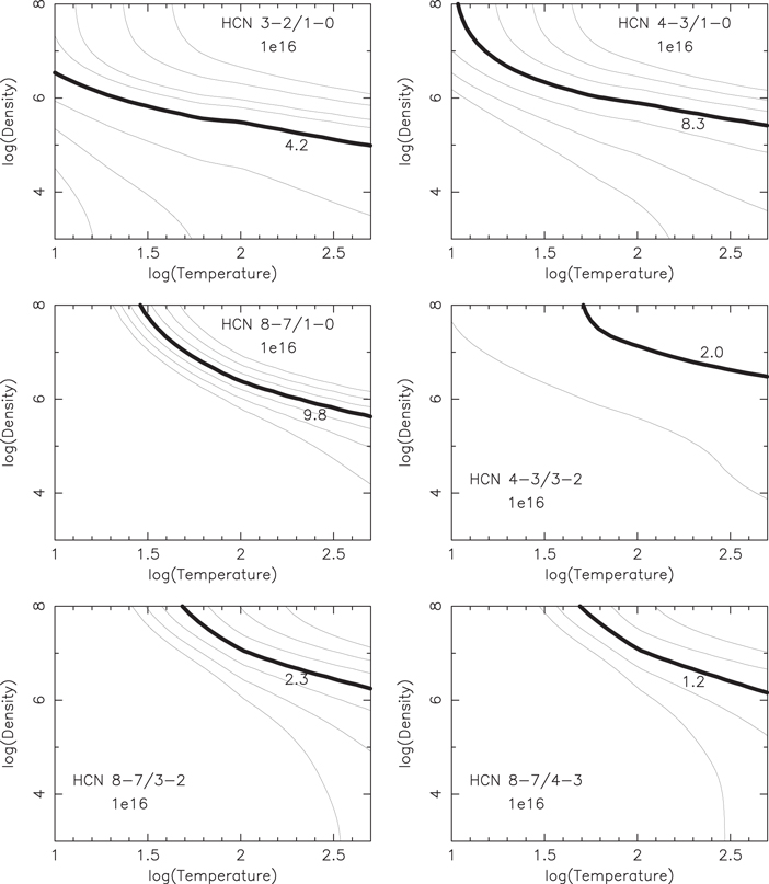
Download figure:
Standard image High-resolution image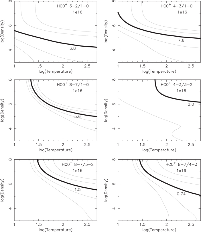
Download figure:
Standard image High-resolution image
Figure 12. RADEX calculation for the column density of 1 × 1016 cm−2 for HCN, HCO+, and HNC. Contours are shown in steps of a factor of 2, with higher (lower) values toward the upper-right (lower-left) direction in all plots. Parameters that reproduce the ratios of the observed fluxes in (Jy km s−1) are shown as thick curved lines with numbers.
Download figure:
Standard image High-resolution imageTable 9. Flux Ratios for HCN, HCO+, and HNC
| J-transition | HCN | HCO+ | HNC |
|---|---|---|---|
| (1) | (2) | (3) | (4) |
| 3–2/1–0 | 4.2 ± 0.6 | 3.8 ± 0.5 | 8.6 ± 1.2 |
| 4–3/1–0 | 8.3 ± 1.2 | 7.6 ± 1.1 | 17.8 ± 2.5 |
| 8–7/1–0 | 9.8 ± 1.4 | 5.6 ± 0.8 | 19.3 ± 4.0 |
| 4–3/3–2 | 2.0 ± 0.3 | 2.0 ± 0.3 | 2.1 ± 0.3 |
| 8–7/3–2 | 2.3 ± 0.3 | 1.5 ± 0.2 | 2.2 ± 0.5 |
| 8–7/4–3 | 1.2 ± 0.2 | 0.74 ± 0.10 | 1.1 ± 0.2 |
Note. Ratios of flux in (Jy km s−1). Column (1): J-transition. Column (2): HCN. Column (3): HCO+. Column (4): HNC. For all flux ratios, 10% absolute calibration uncertainty in individual ALMA observations is included.
Download table as: ASCIITypeset image
Because HCO+ and HNC abundance are estimated to be at least a few times lower than HCN in IRAS 20551−4250 (Section 4.3), we show the same RADEX calculation results in Appendix (Figure 19) for the HCO+ and HNC column density of 3 × 1015 cm−2. The overall trends change little.
In interpreting these results, we must consider two possible caveats. First, the line-emitting volume can differ between the high-J and low-J transition lines. AGNs are typically located at galactic center regions where typical molecular gas density is expected to be higher than that in outer off-nuclear regions, due to nuclear molecular gas concentration. Additionally, in an AGN, the surrounding molecular gas and dust has a strong temperature gradient, such that the temperature at the inner part is higher than that at the outer part. Consequently, dense and warm molecular gas is concentrated in the inner part of the nuclear region, from whence high-J transition lines can be efficiently emitted. More diffuse, low-density cool gas is distributed in more spatially extended regions, which can strongly emit low-J transition lines, but high-J transition line emission is relatively limited. Thus, the probed effective molecular gas volume is very likely to be smaller at higher-J than lower-J transition lines, whereas we assume that both lines come from the same volume in the RADEX calculations. If we focus on the volume of high-J line-emitting molecular gas and compare flux ratios within that volume, then the actual high-J to low-J line flux ratios will be higher than the observed ratios. Thus, the derived temperature and density from the observed flux ratios and RADEX calculations are taken as lower limits for the actual values for the high-J line-emitting molecular gas.
Our second caveat is that, because vibrational transition is not included in our RADEX calculations, infrared radiative pumping is not properly taken into account. For IRAS 20551−4250, it has been quantitatively demonstrated by Imanishi et al. (2016b) and this study (Section 4.3) that infrared radiative pumping plays a role in rotational excitation at v = 0, through the decay from v2 = 1 to v = 0, at least for HCN and HNC, and could realize higher rotational excitation at v = 0 than collisional excitation alone, for a given H2 number density and kinetic temperature. Owing to infrared radiative pumping, lower values of H2 number density and kinetic temperature may suffice to reproduce the observed flux ratios. Thus, the H2 number density and kinetic temperature should be taken as upper limits. This second ambiguity works in opposition to the first, and it is not easy to disentangle the two in a quantitatively reliable manner.
Regarding the first issue, the derived number density and kinetic temperature using low-J lines largely reflect a large volume of spatially extended, low-density, low-temperature molecular gas, resulting in low values. If we compare the flux ratios at high-J transitions only, a small volume of dense and high-temperature molecular gas is preferentially probed, and the derived density and temperature can be high. In Figure 12, we find that the density and kinetic temperature that reproduce the observed flux ratios increase from "J = 3–2 to J = 1–0" to "J = 4–3 to J = 3–2" or "J = 8–7 to J = 4–3" or "J = 8–7 to J = 3–2" for HCN, HCO+, and HNC, i.e., the thick curved line moves from the lower-left to upper-right regions. This is a natural consequence—higher-J lines selectively probe dense and warm molecular gas with a small emitting volume.
In Figure 12, the J = 3–2 to J = 1–0 flux comparison is expected to reflect the largest molecular gas volume, including outer low-density and low-temperature gas. For the kinetic temperature of  > 25 K, the H2 number density of
  =105–106 cm−3 (104–105 cm−3) seems to be required for HCN and HNC (HCO+). The lower required density for HCO+ is reasonable, given that HCO+ has a lower critical density than HCN and HNC under similar line opacity (Meijerink et al. 2007; Greve et al. 2009).
This possible difference among the probed molecular line-emitting volumes can be small if we compare the flux ratios between adjacent J-transitions, such as J = 4–3 and J = 3–2. The typical density and temperature of molecular gas that emits J = 4–3 and J = 3–2 lines are >106 cm−3 and >50 K for HCN, HCO+, and HNC (Figure 12). We thus quantitatively confirm that these J = 4–3 and J = 3–2 emission lines selectively probe dense and warm molecular gas in the close vicinity of energy sources.
The derived density and kinetic temperature that reproduce the observed "J = 8–7 to J = 3–2" and "J = 8–7 to J = 4–3" flux ratios are lower than the "J = 4–3 to J = 3–2" flux ratios for HCN, HCO+, and HNC. This is opposite to the expected trend that the derived density becomes higher when we compare flux ratios at higher-J transition. A plausible explanation for this is that the J = 8–7 emitting volume is substantially smaller than those of J = 4–3 and J = 3–2. This can result in much smaller "J = 8–7 to J = 3–2" and "J = 8–7 to J = 4–3" flux ratios than expected from the same emitting volume assumption, and thereby smaller derived density and kinetic temperature.
The dense molecular mass, derived from the observed HCN J = 1–0 luminosity (Table 6), is estimated to be  , where we adopt the relationship between dense molecular mass and HCN J = 1–0 luminosity,
  = 10×HCN J = 1–0 luminosity [
 (K km s−1 pc2)−1] (Gao & Solomon 2004). Conversely, the hydrogen column density toward the X-ray emitting AGN in IRAS 20551−4250 is
  cm−2 (Franceschini et al. 2003). We here assume that molecular gas distributes spherically and the AGN is located at the center. If all X-ray-obscuring material is in a dense molecular form that is probed with HCN J = 1–0, we obtain the following two relations:


where r (pc) is the radius of the sphere, n (cm−3) is volume averaged gas number density, and  is the mass of molecular hydrogen (=3.3×10⁻²⁴ g). From Equations (6) and (7), we obtain r ∼ 200 (pc) and n ∼ 103 (cm−3). However, if the kinetic temperature is >30 (K), the typical number density of HCN J = 1–0 emitting gas, derived from the observed HCN J = 3–2 to J = 1–0 flux ratio and RADEX calculation, is 105–106 cm−3 (Figure 12). These results can be reconciled if nuclear molecular clouds in IRAS 20551−4250 consist of dense (105–106 cm−3) clumps with a small volume filling factor of 0.1%–1%, as argued by Solomon et al. (1987). The slightly low estimated density of 104–105 cm−3 from HCO+ observations (Figure 12) could be reconciled if HCO+ probes more extended lower-density envelopes of each clump (Imanishi et al. 2016b), because HCO+ emission is observationally found to be more diffuse than HCN (Imanishi et al. 2007; Saito et al. 2015; T. Saito et al. 2017, in preparation). This kind of clumpy molecular structure can naturally explain similar profiles of various molecular emission lines with different line opacity (Solomon et al. 1987), as observed in IRAS 20551−4250 (Imanishi et al. 2016b).
4.5. Molecular Line Flux Ratio
Figure 13 plots the observed HCN-to-HNC and HCN-to-HCO+ flux ratios at J = 1–0, J = 3–2, J = 4–3, and J = 8–7. For J = 3–2 and J = 4–3, line-opacity-corrected intrinsic flux ratios are also shown. In the intrinsic flux ratios, IRAS 20551−4250 deviates even farther away from starburst-dominated regions, suggesting that the line opacity correction, particularly for high-HCN-abundance AGN-containing objects, makes our HCN-based molecular line flux ratio method even more powerful in distinguishing AGNs from starbursts.
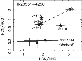
Figure 13. Ratio of HCN-to-HNC flux in (Jy km s−1) (abscissa) and HCN-to-HCO+ flux in (Jy km s−1) (ordinate) at J = 1–0, J = 3–2, J = 4–3, and J = 8–7. While HCN and HCO+ data were obtained simultaneously, HCN and HNC data were not. To calculate the HCN-to-HNC flux ratio, we added 10% absolute flux calibration uncertainty of individual ALMA observations. Observed ratios for IRAS 20551−4250 are shown as filled stars. We assume the HCN flux attenuation from line opacity with a factor of ∼3 at both J = 3–2 and J = 4–3 (minimum side of the estimated range in Section 4.2). In this case, the flux attenuation of HCO+ and HNC is insignificant (a factor of ∼1; Section 4.2). The line-opacity-corrected intrinsic flux ratios at J = 3–2 and J = 4–3 are shown as open stars and are connected to their observed ratios with dotted lines. In addition to IRAS 20551−4250, data at multiple locations of the starburst-dominated galaxy, NGC 1614, are also shown as filled circles for comparison.
Download figure:
Standard image High-resolution imageOn the ordinate, the observed HCN-to-HCO+ flux ratios are comparable at J = 1–0, J = 3–2, and J = 4–3, but are slightly lower than that at J = 8–7. Because the critical density of HCN is higher than HCO+ at individual J-transitions, the higher HCN-to-HCO+ flux ratio at higher J-transition is difficult to explain with collisional excitation under the same line opacity. However, the estimated higher line opacity of HCN reduces its effective critical density with 1/τ. Furthermore, due to higher HCN abundance than HCO+, line-opacity-corrected intrinsic HCN-to-HCO+ flux ratios will be higher than those observed. The intrinsic HCN-to-HCO+ flux ratios at J = 3–2 and J = 4–3 are at least higher than the observed ratio at J = 8–7. Because the line opacity at J = 1–0 is estimated to be higher than J = 8–7 with RADEX under the parameter range of  cm−3,
cm−3,  K,
K,  cm−2, and Δv = 300 km s−1, the intrinsic HCN-to-HCO+ flux ratio at J = 1–0 will move to the upper side more than at J = 8–7. Both of these factors could help to explain the result.
On the abscissa, the observed HCN-to-HNC flux ratio at J = 1–0 is higher than those at J = 3–2, J = 4–3, and J = 8–7. Figure 14 is the plot of the "high-J to low-J" flux ratios for HCN, HCO+, and HNC, where the combination of "J = 3–2 to J = 1–0," "J = 4–3 to J = 1–0," "J = 8–7 to J = 1–0," "J = 4–3 to J = 3–2," "J = 8–7 to J = 3–2," and "J = 8–7 to J = 4–3" are selected. The actual ratios are summarized in Table 9. We see a trend that the ratios are a factor of ∼2 higher for HNC than HCN and HCO+ for the first three combinations (including J = 1–0 as the low-J transition), but comparable for the latter three combinations (not including J = 1–0). HCN and HNC have comparable critical densities at individual J-transition under a similar line opacity (Greve et al. 2009). The derived higher HCN opacity (Sections 4.2 and 4.3) will make the effective HCN critical density lower than HNC, in which case the "high-J to low-J" flux ratios for HNC are expected to be lower than those for HCN, when collisional excitation is considered. This is opposite to the trends observed in Figure 14.

Figure 14. Flux ratios of high-J to low-J transition lines for HCN, HCO+, and HNC. Fluxes are in units of (Jy km s−1).
Download figure:
Standard image High-resolution imageThe excitation temperatures of rotational J-transition at v = 0 are summarized in Table 8, where the differences of beam sizes are not considered, to be consistent with our previous calculations (Imanishi et al. 2016b). This assumes that the intrinsic emission size is the same among HCN, HCO+, and HNC, and is smaller than the beam sizes in all observations. The rotational excitation temperatures within v = 0 are slightly higher for HNC than for HCN (Table 8).
We suggest that the following two mechanisms could help reduce the discrepancy between observations and predictions. First, we find from our RADEX calculations that, at high density ( cm−3) and temperature (
 K), a maser phenomenon occurs at J = 1–0 first for HCN and HCO+, and then later for HNC. For example, for the column density of 1 × 1016 cm−2, Δv = 300 km s−1, and
  = 1–3 × 106 cm−3, the maser phenomenon is predicted to occur at
  K for HCN J = 1–0, but only at
  K for HNC J = 1–0. Further, with
  cm−3, HCN J = 1–0 shows the maser phenomenon at
  K, but HNC J = 1–0 does not. The maser phenomenon could boost J = 1–0 emission. If the maser occurs only for HCN J = 1–0, but not for HNC J = 1–0, under some parameter range, the "high-J to J = 1–0" flux ratios for HCN could be smaller than HNC. HCO+ J = 1–0 also starts to show the maser phenomenon earlier than HNC from lower density and temperature. The higher values of "high-J to J = 1–0" flux ratios for HNC than HCO+ could also be explained by the maser phenomenon in some parameter range.
Our second scenario is infrared radiative pumping. In IRAS 20551−4250, it is calculated that the infrared radiative pumping rate is higher for HNC than for HCN and HCO+ (Section 4.3 and Imanishi et al. 2016b). This could boost high-J HNC emission more than HCN and HCO+, through decay back from v2 = 1 to v = 0. Given that this infrared radiative pumping is estimated to play a role in IRAS 20551−4250, at least for HCN and HNC (Section 4.3), its effect must be evaluated in an appropriate manner.
4.6. Inclusion of Infrared Radiative Pumping
Our ultimate goal is to quantitatively estimate (1) what fraction of molecular excitation at individual J-transition levels is due to collision and infrared radiative pumping, and (2) the increase of molecular line fluxes at individual J-transitions, brought by infrared radiative pumping, when compared to collisional excitation alone. However, this is difficult to achieve with currently available data, because of a large freedom of parameters for collisional excitation. First, the possibly different emitting volumes at different J-transitions (Section 4.4) are not constrained in a meaningful manner. Next, the typical temperature and density probed by different J-transition lines are different (Section 4.4), so different numbers of multiple temperature and density components need to be taken into account when we compare flux ratios among different J-transition lines. We thus investigate quantitatively how infrared radiative pumping reproduces the observed trend of higher values of "high-J to low-J" flux ratios for HNC than HCN shown in Figure 14, by fixing molecular gas physical parameters to canonical values. We use MOLPOP (Elitzur & Asensio Ramos 2006), which handles the exact solution of radiative transfer problem in multi-level atomic systems. The ∼3 K cosmic microwave background radiation is always included in MOLPOP. The LVG method is prepared as an option, and we adopt it to compare the output with our RADEX calculation results. We have quantitatively confirmed that, under LVG, both MOLPOP and RADEX outputs about molecular line flux ratios among J = 1–0, J = 3–2, J = 4–3, and J = 8–7 agree within 20–30% for various H2 number density, H2 kinetic temperature, and molecular column density divided by line width.
To calculate the role of infrared radiative pumping, we require Einstein A coefficient values for vibrational (v)-rotational (J) transitions between (v2, J) = (1, J) and (0, J ± 1 or J). We find the required information for HCN and HNC, but not for HCO+, in the GEISA database (Jacquinet-Husson et al. 2016). We thus perform this calculation for HCN and HNC. Collision rates between J-transition levels at v2 = 1 are not available, so we tentatively adopt the same values as v = 0. Because vibrational-rotational transitions are much faster than the transitions between J-levels within v2 = 1 (Imanishi et al. 2016b), possible small ambiguities in the collision rates at v2 = 1 do not significantly affect our final results. Collisional transitions between v2 = 1 and v = 0 are also not taken into account, due to their very large energy gaps.
In MOLPOP, we first set  cm−3,
cm−3,  (K), Δv = 300 km s−1, and the HCN and HNC column density of 1016 cm−2, in order to calculate molecular line fluxes by collisional excitation. We confirm that the maser phenomenon does not happen at J = 1–0. We choose the small side of the estimated density range for HCN and HNC,
  cm−3 for our calculations, because the maser phenomenon happens at higher
  values, which complicates interpretations. We then add infrared radiation at 5–30 μm in the power-law form of
  (Jy) = 0.0024 × λ(μm)2.0 (the dashed straight line in Imanishi et al. (2016b)). In this form, the number of infrared photons at ∼22 μm is larger than at 12–14 μm. The integrated luminosity between 5–30 μm is estimated to be
  at a distance of 187 Mpc (z = 0.043). Plane-parallel geometry is adopted, and the infrared 5–30 μm radiation source is placed at 30 pc and 100 pc from the molecular gas. We then investigate if the high-J to low-J flux ratios of HNC are higher than HCN, particularly for "J = 3–2 to J = 1–0," "J = 4–3 to J = 1–0," and "J = 8–7 to J = 1–0," as observed in Figure 14. Figure 15(a) plots the values of "high-J to low-J flux ratio of HNC, divided by the same ratio of HCN" in the ordinate. Because the infrared radiative pumping effects are calculated to be higher for HNC than HCN, the high-J to low-J flux ratios for HNC are expected to increase more than those for HCN, by the inclusion of infrared radiation. Namely, the values in the ordinate are expected to be higher in the case of stronger infrared radiation than the case with no infrared radiation (i.e., collisional excitation only). We find that the inclusion of infrared radiative pumping better reproduces the observed trend of higher values of "high-J to low-J flux ratios" for HNC than HCN, for the combinations of "J = 3–2 to J = 1–0," "J = 4–3 to J = 1–0," and "J = 8–7 to J = 1–0" observed in Figure 14.

Figure 15. Quantitative investigation of the effect of infrared radiation on high-J to low-J flux ratios for HCN and HNC, using the MOLPOP software (Elitzur & Asensio Ramos 2006). The ordinate is the values of "high-J to low-J flux ratio of HNC, divided by the same ratio of HCN." The combination of "high-J to low-J" is "J = 3–2 to J = 1–0," "J = 4–3 to J = 1–0," "J = 8–7 to J = 1–0," "J = 4–3 to J = 3–2," "J = 8–7 to J = 3–2," and "J = 8–7 to J = 4–3." The values in the case of no external radiation (i.e., collisional excitation alone) are set to unity for all high-J to low-J combinations. Thus, the ordinate corresponds to the increased factor of the values by the inclusion of infrared radiation. The molecular gas parameters are  number density
  cm−3,
cm−3,  kinetic temperature
  K, and velocity width Δv = 300 km s−1. The ∼3 K cosmic microwave background emission is included. Open circles indicate no external radiation. Filled stars show an infrared radiating energy source with
  (Jy) = 0.0024 × λ(μm)
 that is placed at 30 pc from the molecular gas. Filled squares are the same infrared radiating energy source placed at 100 pc from the molecular gas. (a) The column density is 1016 cm−2 for both HCN and HNC. (b) The HCN and HNC column densities are 1016 cm−2 and 3 × 1015 cm−2, respectively.
Download figure:
Standard image High-resolution imageIn Figure 15(b), we display a similar plot, but with a factor of ∼3 smaller HNC column density than HCN, as indicated in Section 4.3. Because an additional parameter is introduced, the behavior becomes complicated, but the general trend of enhanced high-J to J = 1–0 flux ratios for HNC, as compared to HCN, is observed. We thus argue that the observed trend in IRAS 20551−4250 can be largely accounted for by infrared radiative pumping.
Although collisional excitation is usually adopted to interpret the observed molecular J-transition emission line fluxes in galaxies, it has been widely argued that the infrared radiative pumping mechanism can play an important role in AGN-containing galaxies, because AGNs can emit strong mid-infrared 5–30 μm continuum photons due to AGN-heated hot dust grains. In this AGN-containing ULIRG, IRAS 20551−4250, we have demonstrated that the infrared radiative pumping indeed plays a role for molecular rotational J-level excitation, at least for HCN and HNC, which suggests that this is the case in other AGN-containing ULIRGs as well. However, in general ULIRGs, the similar estimates of the infrared radiative pumping effects, through the v2 = 1f emission line flux measurements, are prohibitively difficult because HCN J = 3–2 and J = 4–3 emission lines at the v2 = 1 level are spectrally highly overlapped with the nearby, much brighter HCO+ J = 3–2 and J = 4–3 emission lines at the v = 0 level, respectively (Aalto et al. 2015b; Imanishi et al. 2016c). IRAS 20551−4250 is unique in that, thanks to its small observed molecular emission line widths, the flux estimates of the HCN v2 = 1f J = 3–2 and J = 4–3 emission lines are possible, by clearly separating from the bright HCO+ (v = 0) emission lines. Further detailed investigations of IRAS 20551−4250 with additional emission lines at v = 0 and v2 = 1 will help better constrain the quantitative role of infrared radiative pumping in this ULIRG as well as other AGN-containing ULIRGs.
4.7. Infrared-to-Radio Spectral Energy Distribution
Figure 16 shows the spectral energy distribution (SED) of IRAS 20551−4250 in the infrared and radio. The q-value, defined as the far-infrared-to-radio flux ratio, is q ∼ 2.7 (Table 1). This is not smaller than for starburst-dominated galaxies and many radio-quiet AGNs (q ∼ 2.3–2.4) (Condon et al. 1991; Barvainis et al. 1996; Crawford et al. 1996; Roy et al. 1998), suggesting that the infrared-to-radio SED of IRAS 20551−4250 is an example of a radio-quiet AGN and starburst composite.

Figure 16. Infrared-to-radio spectral energy distribution. Filled stars: Our ALMA data, including Imanishi et al. (2016b). In band 7 (275–373 GHz), both our J43a and J43b continuum measurements in ALMA Cycle 2 (Table 3) are plotted, but overlap in the figure. Our ALMA Cycle 0 continuum measurements in band 7 (Imanishi & Nakanishi 2013b) are not plotted. Filled squares are from the literature. Near-infrared 1–3 μm data are from 2MASS. Infrared 10–200 μm data are from IRAS and ISO photometry (Spinoglio et al. 2002; Brauher et al. 2008). Radio 1.4 GHz and 4–9 GHz data are from Condon et al. (1996) and Georgakakis et al. (2000), respectively. Radio 843 MHz data are from SUMSS (Sydney University Molonglo Sky Survey, Version 2.1, 2008).
Download figure:
Standard image High-resolution imageContinuum data points in ALMA bands 7 (275–373 GHz) and 9 (602–720 GHz) are well-fitted to extrapolation from the infrared dust thermal radiation at 2000–7500 GHz (40–150 μm). ALMA band 3 (84–116 GHz) continuum data points roughly agree with the extrapolation from lower-frequency synchrotron emission. The thermal free–free emission from starburst regions in IRAS 20551−4250 is also present (Imanishi & Nakanishi 2013b; Imanishi et al. 2016b), but mainly contributes to the frequency range at the minimum flux density (∼200 GHz), due to its relatively flat spectral shape. Overall, continuum flux measurements with our ALMA data in the (sub)millimeter wavelength range are consistent with those at other wavelengths taken with other observing facilities, further confirming that most activity (AGN and/or starburst) in IRAS 20551−4250 is spatially compact, and their emission is well-recovered with our ALMA interferometric data.
5. Summary
We conducted ALMA band 3, 6, 7, and 9 observations of the buried-AGN-hosting ULIRG, IRAS 20551−4250, in Cycles 2, 3, and 4. When our new data were combined with our previously collected ALMA data, we obtained information on flux and its sensitive upper limit for J = 1–0, J = 3–2, J = 4–3, and J = 8–7 emission lines of HCN, HCO+, HNC, CO J = 3–2; vibrationally excited (v2 = 1f) J = 3–2 and J = 4–3 emission lines of HCN, HCO+, and HNC; v2 = 1f J = 8–7 emission lines of HCN and HNC; J = 3–2 emission lines of isotopologue H13CN, H13CO+, and HN13C; and some other serendipitously detected emission lines. From our previous ALMA observations of HCN, HCO+, and HNC at J = 3–2, and calculations of infrared radiative pumping, it had been argued that HCN abundance was higher than HCO+ and HNC, and that an infrared radiative pumping played a role in molecular gas rotational (J) excitation at the vibrational ground level (v = 0) in IRAS 20551−4250. By adding our new ALMA data, we found the following main results.
- 1.We detected v2 = 1f emission lines at J = 4–3 for HCN and HNC, but not for HCO+, in the same manner as our previous J = 3–2 observations. HCO+ v2 = 1f fluxes are smaller than HCN v2 = 1f and HNC v2 = 1f fluxes at both J = 3–2 and J = 4–3. The estimated vibrational excitation temperature from J = 4–3 supported our previous argument, based on J = 3–2 data, that the infrared radiative pumping plays a role in rotational excitation at v = 0, at least for HCN and HNC.
- 2.There are possible signatures of v2 = 1f J = 8–7 emission lines of HCN and HNC in our ALMA band 9 spectrum; however, their detection significance is at most ∼3σ, in both their integrated intensity (moment 0) maps and Gaussian fits in the spectra. Confirmation with deeper data will be necessary for further discussion of these lines.
- 3.The J = 4–3 fluxes of HCN, HCO+, and HNC at v2 = 1f and v = 0 can be explained by a higher HCN abundance than HCO+ and HNC, as was previously argued from J = 3–2 data.
- 4.The comparison of fluxes between HCN, HCO+, and HNC and their isotopologues (H13CN, H13CO, and HN13C) at J = 3–2 also suggests higher flux attenuation by line opacity for HCN than for HCO+ and HNC, supporting the above higher HCN abundance scenario than HCO+ and HNC.
- 5.Line-opacity-corrected intrinsic molecular line flux ratios among HCN, HCO+, and HNC were derived at J = 3–2 and J = 4–3. We confirmed that IRAS 20551−4250 has higher intrinsic HCN-to-HCO+ and HCN-to-HNC flux ratios than the observed ratios. The difference from starburst-dominated regions was even larger if the intrinsic ratios are used for IRAS 20551−4250.
- 6.The bright CO J = 3–2 emission line enabled us to probe the dynamical properties of spatially extended molecular gas in detail, and showed a dynamically distinct region at the southwestern part of the nucleus, compared to overall rotational motion. Our molecular observations support the scenario that some past merger event occurred in IRAS 20551−4250.
- 7.A broad (FWHM ∼ 500 km s−1) emission line component was detected in the bright CO J = 3–2 emission line, which we interpret to be caused by molecular outflow activity in this galaxy. We estimate a molecular outflow mass
 , a molecular outflow rate ( yr−1), a molecular outflow kinetic power of AGN luminosity (), and a molecular outflow momentum rate .
 - 8.We conducted RADEX calculations and derived H2 number density and kinetic temperature that reproduce the observed flux ratios at different rotational J-transition lines of HCN, HCO+, and HNC at v = 0, by collisional excitation. The derived number density and kinetic temperature tend to be higher when we use higher-J transition lines, supporting the expectation that higher-J transition lines preferentially probe higher-density and higher-temperature molecular gas in more compact areas. The comparison between J = 3–2 and J = 1–0 suggests that the typical molecular gas density that emits the HCN J = 1–0 emission line is ∼105–106 (cm−3). The X-ray-absorbing hydrogen column density and estimated mass of dense molecular gas from HCN J = 1–0 luminosity suggest that the volume averaged number density and size of HCN J = 1–0 emitting molecular gas are ∼103 (cm−3) and ∼200 (pc), respectively. We infer that the molecular clouds in the IRAS 20551−4250 nucleus are in a clumpy form, in which dense clumps with ∼105–106 (cm−3) occupy 0.1–1% of the total volume of the nuclear molecular gas.
- 9.From our J = 8–7, J = 4–3, J = 3–2, and J = 1–0 data of HCN, HCO+, and HNC, higher rotational excitation was seen for HNC than for HCN or HCO+. This is difficult to explain with only collisional excitation, due to the estimated effective critical density of HNC being higher than those of HCN and HCO+. Infrared radiative pumping could explain this result, because HNC has higher infrared pumping efficiency than HCN or HCO+, due to a larger amount of infrared photons at ∼22 μm (wavelength for vibrational-rotational transitions between v = 0 and v2 = 1 for HNC) than at 12–14 μm (those for HCN and HCO+). Apart from the vibrational excitation temperature, this is another indication that infrared radiative pumping is at work in IRAS 20551−4250. Given that Einstein A coefficients for vibrational-rotational transitions are available for HCN and HNC, we performed quantitative calculations of the effects of the infrared radiative pumping process for HCN and HNC, using the MOLPOP software. We found that the observed higher HNC rotational excitation was largely reproduced if an energy source with observationally constrained infrared spectral shape was placed at 30–100 pc from the molecular gas.


IRAS 20551−4250 is a unique ULIRG, in that the small observed molecular emission line widths allow us to clearly separate the HCN v2 = 1f J = 3–2 and J = 4–3 emission lines from the nearby, much brighter HCO+ (v = 0) J = 3–2 and J = 4–3 emission lines. Thus, we can investigate both molecular line fluxes at the v2 = 1 level and the effects of infrared radiative pumping, with small quantitative uncertainty. Given that the infrared radiative pumping can have a significant effect on other AGN-containing ULIRGs, but its quantitative estimate is more difficult due to the spectral overlap between HCN v2 = 1f and HCO+ v = 0 emission lines at J = 3–2 and J = 4–3, further detailed investigations of IRAS 20551−4250 will provide an important clue to help understand how the infrared radiative pumping contributes to molecular rotational J-transition line fluxes at v = 0, in addition to the usually assumed collisional excitation, in AGN-containing ULIRGs.
We thank the anonymous referee for his/her useful comments, which greatly helped us to improve the clarity of this manuscript. We are grateful to Dr. H. Nagai, A. Kawamura, and F. Egusa for their kind help regarding ALMA data retrieval and reduction. We are thankful to Dr. M. Elitzur and A. Asensio Ramos for their kind advice about the use of the MOLPOP code. M.I. was supported by JSPS KAKENHI Grant Number 23540273, 15K05030 and the ALMA Japan Research Grant of the NAOJ Chile Observatory, NAOJ-ALMA-0001, 0023, 0072. T.I. is thankful for a fellowship received from the Japan Society for the Promotion of Science (JSPS). This paper makes use of the following ALMA data: ADS/JAO.ALMA#2013.1.00033.S, #2015.1.00028.S, and #2016.1.00051.S. ALMA is a partnership of ESO (representing its member states), NSF (USA), and NINS (Japan), together with NRC (Canada), NSC, ASIAA (Taiwan), and KASI (Republic of Korea), in cooperation with the Republic of Chile. The Joint ALMA Observatory is operated by ESO, AUI/NRAO, and NAOJ. Data analysis was in part carried out on the open-use data analysis computer system at the Astronomy Data Center, ADC, of the National Astronomical Observatory of Japan. This research has made use of NASA's Astrophysics Data System and the NASA/IPAC Extragalactic Database (NED) which is operated by the Jet Propulsion Laboratory, California Institute of Technology, under contract with the National Aeronautics and Space Administration.
Appendix:
Integrated intensity (moment 0) maps of selected serendipitously detected faint emission lines are displayed in Figure 17. Figure 18 shows spectra around these lines and best Gaussian fits, except for "SO2 + SO" in Figure 17, because two lines overlap at close frequency (Figure 2(c)). Figure 19 shows our RADEX calculations to reproduce the observed molecular line flux ratios, in the case of HCO+ and HNC column density of 3 × 1015 cm−2.
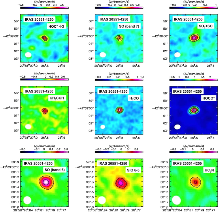
Figure 17. Integrated intensity (moment 0) maps of the serendipitously detected faint molecular lines in IRAS 20551−4250. Molecular lines detected in ALMA band 7 observations are displayed first (six images), followed by those in band 6 (three images). The contours represent 4σ, 5σ, and 6σ for HOC+ J = 4–3; 4σ, 6σ, and 8σ for SO (band 7); 4σ, 8σ, and 12σ for SO2+SO; 4σ and 6σ for CH3CCH; 5σ, 10σ, and 20σ for H2CO; 10σ, 20σ, 30σ, and 40σ for HOCO+; 3σ and 8σ for SO (band 6); 3σ and 5σ SiO J = 6–5; and 3σ and 6σ for HC3N J = 27–26. The 1σ levels are different for different molecular lines, and are summarized in Table 4. Beam sizes are shown as filled circles in the lower-left region. The displayed areas differ depending on the beam size.
Download figure:
Standard image High-resolution image
Figure 18. Spectra around selected serendipitously detected faint molecular emission lines. The abscissa is optical LSR velocity ( (
( ), and the ordinate is flux in (mJy beam−1). Best Gaussian fits are overplotted with solid curved lines.
Download figure:
Standard image High-resolution image
Download figure:
Standard image High-resolution image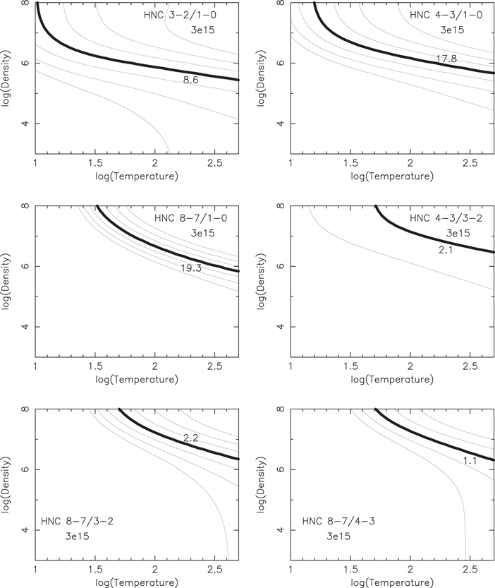
Figure 19. RADEX calculation for the column density of 3 × 1015 cm−2 for HCO+ and HNC. Contours are shown in steps of a factor of 2, with higher (lower) values in the upper-right (lower-left) direction in all plots. Parameters that reproduce the ratios of the observed fluxes in (Jy km s−1) are shown as thick curved lines with numbers.
Download figure:
Standard image High-resolution image
Footnotes
- 4
A vibrationally excited J = 1–0 line is not present.
- 5
The J = 4–3 to J = 3–2 flux ratios for HCN, HCO+, and HNC are all comparable to each other (Imanishi et al. 2016b). Given that the molecular population is typically dominated by low J levels at J < 5, this assumption is reasonable for IRAS 20551−4250.