


Abstract
Improving our capability to interpret observations of cometary dust is necessary to deepen our understanding of the role of dust in the formation of comets and in altering the cometary environments. Models including dust grains are in demand to interpret observations and test hypotheses. Several existing models have taken into account the gas–dust interaction, varying sizes of dust grains and the cometary gravitational force. In this work, we develop a multi-fluid dust model based on the BATS-R-US code. This model not only incorporates key features of previous dust models, but also has the capability of simulating time-dependent phenomena. Since the model is run in the rotating comet reference frame, the centrifugal and Coriolis forces are included. The boundary conditions on the nucleus surface can be set according to the distribution of activity and the solar illumination. The Sun revolves around the comet in this frame. A newly developed numerical mesh is also used to resolve the real-shaped nucleus in the center and to facilitate prescription of the outer boundary conditions that accommodate the rotating frame. The inner part of the mesh is a box composed of Cartesian cells and the outer surface is a smooth sphere, with stretched cells filled in between the box and the sphere. Our model achieved comparable results to the Direct Simulation Monte Carlo method and the Rosetta/OSIRIS observations. It is also applied to study the effects of the rotating nucleus and the cometary activity and offers interpretations of some dust observations of comet 67P/Churyumov–Gerasimenko.
Export citation and abstract BibTeX RIS
1. Introduction
Dust and gas in comets are believed to have preserved the building material of the early solar system. Unfortunately, it is difficult to obtain the bulk composition of both dust and gas in the nuclei of a large number of comets by remote observations. As the apparent dust-to-gas ratio in the coma is better accessible for remote and in situ observations than the composition of dust and gas, and is no less critical to our understanding of the formation of the solar system, models that are able to interpret the dust observations, and can better constrain this quantity, are desirable.
Dust grains prevail in cometary environments and have various compositions, i.e., water ice, SiO2, Mg, Fe (Kissel et al. 1986a, 1986b; Hanner et al. 1990; Lellouch et al. 1998). The size of dust grains ranges from sub-micron to meters, which affects the behavior of dust grains (Mukai et al. 1986). For example, one millimeter-sized grain reflects more visible light than a micron-sized grain because of its larger geometric cross section. Smaller grains can be accelerated by gas more efficiently because of their higher cross-section-to-mass ratio, assuming grains of all sizes have the same bulk density. Since one type of observation or one instrument covers only part of the size range, a reasonable estimation of the size distribution is needed to obtain the total dust loss rate or the dust-to-gas production ratio. However, the problem can be more complicated, as grains' fragmentation and sublimation may also alter the size distribution.
When it comes to interpreting dust observations, more factors have to be considered. Since dust grains are subject to the gas drag, the gas activity must be taken into account. Therefore, heterogeneity of the outgassing from the rotating nucleus surface with the variation of solar illumination can lead to complex dust behavior. Depending on the sum of the gas drag, solar radiation pressure, and the gravity of the comet, some dust grains may escape with the gas, some orbit around the nucleus, and some fall back to the surface. When the escaping dust grains are far from the comet, usually beyond 104 km, where the anti-sunward radiation pressure is equal to or larger than the gas drag force, they will get pushed back toward the nucleus (Fougere et al. 2013). Radiation pressure also affects the maximum liftable grain sizes right at the nucleus (Tenishev et al. 2011). On comet 103P/Hartley 2, sublimating icy grains serve as an extended source, supplying most water gas in the coma (Fougere et al. 2013). The initial velocity of the gas just sublimated from the grains tends to be slower than the ambient gas that has already been accelerated. Since the dust grains often have a higher temperature than the ambient gas, the sublimated gas can also heat the coma. Consequently, an extended distribution of grains containing volatiles or semi-volatiles can greatly alter the gas velocity and temperature profile of the coma (Fougere 2014). However, there is no evidence for a significant extended source for comet 67P, thus this effect is not considered in this work.
In addition, dust grains can also get charged by photo-electrons generated by solar radiation at the surface, impact from ions and electrons in the solar wind, and electron attachment. Charged dust grains are subject to an additional force caused by the electromagnetic field in the cometary plasma. In some cases, the electromagnetic force can become the dominant factor and thus the charged dust dynamics is more similar to ions in plasma than other neutral dust grains. The collective behavior of charged dust can be very complicated, especially when the charging effects of spacecraft can have an effect on the movement of charged grains. As a result, all kinds of dust grains populate the cometary environment, making it challenging to understand the observational data.
In this work, we will focus on the neutral dust grains and the charged dust is not considered. Several models have been developed to study the neutral dust–gas interaction, which can be divided into two groups. One group treats the gas and dust as fluids and solves Euler equations or Navier–Stokes equations for density, velocity, and pressure (e.g., Kitamura 1986; Crifo 1995); the other one represents dust and gas with particles and keeps track of the velocities and locations of each particle, the statistics of which can also provide the same macro-quantities as fluid models. The Direct Simulation Monte Carlo (DSMC) method is one example among the second group and has demonstrated its advantages over fluid models in studying dust grains' behavior (Tenishev et al. 2011; Marschall et al. 2016), because (1) it is able to model a continuous spectrum of dust sizes, while fluid models can only do several discrete sizes; and (2) it can model dust grain trajectories crossing each other but fluid models cannot. However, when it comes to simulating time-dependent three-dimensional phenomena on large length scales, where the transportation timescale becomes at least considerable to the rotation period of the comet, fluid models can be more computationally feasible than DSMC models.
In this work, we developed a cometary dust model, which not only has key features of fluid dust models, but also applies a newly developed numerical mesh to resolve the irregular shape of the nucleus and to accommodate the rotating nucleus. In the following sections, we will first compare our model with the DSMC approach and then study the effects of the cometary rotation and activity on dust grains' behavior using a real-shaped nucleus. A comparison between model results and corresponding observations by Rosetta is also preformed.
2. Model Description
Our model is based on the BATS-R-US (Block-Adaptive Tree Solar wind Roe-type Upwind Scheme) code (Powell et al. 1999; Tóth et al. 2012) in the Space Weather Modeling Framework (SWMF) developed by the University of Michigan. It treats H2O gas and dust grains of 6 sizes, every decade from 10−7 to 10−2 m, as different fluids. Each fluid has its own continuity equation and momentum equation. Unlike gases, solid dust grains do not have energy equations, though they do have grain temperatures calculated from thermal equilibrium with Sun light. As our studies are limited to the vicinity of the comet, within a distance less than 100 km to the nucleus, the photodissociation of H2O with a length scale of about 105 km is neglected (Shou et al. 2016). Compared to the gas drag force, the radiation pressure does not make a significant difference near the nucleus (Crifo et al. 2003; Tenishev et al. 2011). Since our target, comet 67P/Churyumov–Gerasimenko, is a weak comet with a peak production rate of about 3.5 × 1028 s−1 near perihelion (Hansen et al. 2016), the heating effect of dust grains on the gas energy balance is not included either (Crifo et al. 2005). But the effect of gas drag is taken into account by introducing a corresponding source term to the momentum equations of dust grains. The term can be expressed as  , where the drag coefficient Cd is approximated as 2,
  is the water mass density, ndust is the dust number density, a is the radius of the dust grain assuming sphericity, and
  and
and  are the velocities of water and dust grains. The bulk density of all dust grains is assumed to be 103 kg/m3. When the model is run in the co-rotating frame, the fictitious forces, i.e., centrifugal and Coriolis forces, are included.
3. Boundary Conditions
In the first study we do a comparison with the DSMC approach by Tenishev et al. (2011) and thus use a spherical nucleus with a radius of 2 km. The models at four heliocentric distances are run in the inertial frame. We also assume a non-rotating body and the solar illumination does not change. The gas flux and temperature are fixed at the surface of the body. The inner boundary conditions of the four cases are compatible with those in Tenishev et al. (2011) derived from Davidsson & Gutiérrez (2004) and Davidsson & Gutiérrez (2005). The surface temperature profile and the water flux distribution can be found in Tenishev et al. (2011). The temperature and the water flux on the surface are governed by the solar zenith angle (SZA). At the lowest SZA, the temperature and the gas flux reach their maxima. As the SZA increases, both temperature and flux decrease until a critical SZA is reached. It is assumed that regions beyond that SZA are at the cometary local night, and all have the lowest temperature and the lowest flux.
The dust flux is assumed to be proportional to the H2O flux and the multiplier is given by the ratio of dust-to-gas production rates. The dust-to-gas mass production ratio used in the first part of this study is 0.8, which is the same number used by Tenishev et al. (2011). In order to ensure the dust-to-gas mass production ratio at the boundary is exactly the constant we set, the initial velocities of all dust grains are set to be a fixed fraction of water velocity. As mass flux is the product of velocity and mass density, if the dust velocity is zero, it is very difficult for the fluid model to control the flux ratio. Therefore, the initial velocities of all dust grains are set to be less than 10% of the escape velocity at 10−4 times the H2O gas velocity and the gas drag is then allowed to lift and accelerate the dust. The number density of dust grains follows a power-law relationship, with an exponent of −3: , where a is the radius of the dust grain. Since by definition all particles are initially started at the same small velocity the local density distribution as well as the normally used dust production flux distribution have the same power law at the surface. The gas–dust physics then naturally produces the appropriate dust fluxes as a function of particle size. All of the steady-state runs are performed on a spherical grid. The highest resolution is applied to the region close to the nucleus, where it is about 0.02 km in the radial direction and 2
 8 and 14 in the polar and azimuthal directions. Floating boundary conditions, which ensure a zero gradient in computed variables, are applied to the outer boundaries at a cometocentric distance of 85 km, where the resolution in radial direction is about 2.5 km.
In Section 4.2 the actual shape of comet 67P/Churyumov–Gerasimenko is used to study the effects of a rotating nucleus on dust grain dynamics. The geometry of the nucleus affects not only the gravity near the nucleus, but also the surface area that is illuminated by the Sun, notably due to the concavity of the nucleus shape and the apparition of self-shadowing effects. The activity map of H2O obtained by Fougere et al. (2016), combined with the changing SZA, provides the boundary condition on the surface. The H2O distribution map was constrained by the ROSINA/DFMS data from 2014 August to 2015 May, and the map shows increased H2O activity at high northern latitudes. At some regions on the nucleus, the surface normal can be perpendicular to the direction of the gravity, which allows very large dust grains to leave the surface. At other locations where the gas flux is low and the gravity is large, heavy dust grains cannot be lifted by the gas. Similarly, there would be locations where solar radiation pressures help or prevent dust grains from being lifted. However, solar radiation pressure is not included in this model. The maximum size of liftable dust grains can be calculated by the local flux and the gravity force in the normal direction of the surface, which is expressed as  , where z is the local gas mass production rate, uout is the normal velocity of gas,
  is the bulk density of dust grains, (1 g cm−3 is used in this work and is somewhat arbitrary), and gnormal is the normal component of the gravitational acceleration. If one dust fluid has a size larger than the local maximum liftable size, the density of that fluid is set to a small number, due to the fluid approach prohibiting vacuum, and the velocity is set to zero for dust particles that cannot be lifted. It should be noted here that the gravity field is computed using the real-shaped nucleus with homogeneous density. In addition, the model is run in the co-rotating frame of the comet to fully account for the rotational effects. Case 1 applies an imaginary boundary condition when the Sun is rotating with the comet at the same rate, to illustrate the effect of a fixed boundary condition. Case 2 is more realistic, with a revolving Sun in the rotating frame, which results in a time-varying boundary condition. The boundary condition is updated as the subsolar point on the nucleus changes its longitude every 15°, which corresponds to a time of about 30 minute for comet 67P. Our setup may update less frequently than the real solar and cometary condition changes, but it is an approximation that works well for the purposes of our theoretical study.
In Section 4.3, we compare our time-dependent model results with the dust images observed by the Rosetta/OSIRIS Wide Angle Camera (WAC). This study uses the scaled water activity map in Fougere et al. (2016), but applies real solar latitudes and longitudes at the time when OSIRIS measurements were made.
3.1. Treatment of Returning Dust Grains
Because of the varying surface boundary conditions, there are dust grains of the same size that can be lifted in some regions on the comet but cannot in other regions. Some of the lifted grains are carried away by the gas from the nucleus forever, but gravity becomes important for slow-moving particles in particular. In the extreme case dust particles are not accelerated beyond the escape velocity and thus fall back. The ones falling back are called returning dust grains and will end up resting on the surface region unless the boundary condition changes to lift them again.
The returning dust grains can be treated in a straightforward way with the DSMC approach, but require special considerations in a fluid model. In the DSMC model, before any particles are injected into the computational domain, a vacuum initial condition can exist. However, a vacuum initial condition is not allowed in the fluid model, and the density and the pressure of any fluid should have positive values, anywhere in the computational domain and at any time. The initial states of all fluid densities are often assigned a small positive number. This limitation can have artificial effects on dust fluids with large sizes, especially for those fluids on the nightside that cannot be lifted. In the numerical simulation, the small amounts of heavy dust that are set in the whole domain from the very beginning will be attracted to the nucleus and accelerated by the gravity, resulting in a density pile-up and a relatively high speed near the nucleus about 2 km from the origin. To minimize the numerical artificial effects, we prescribe a "free falling zone," which is a small zone compared to the whole domain. Inside the "free falling zone," returning dust grains or grains of unliftable sizes are allowed to fall back to the comet. Outside of that zone, if dust grains there cannot be dragged away by the gas, they will stay fixed at where they are. This treatment prohibits any particles outside the zone returning to the nucleus. The "free falling zone" is within 15 km from the origin in this work.
3.2. The "Roundcube" Mesh
There are two ways to study the effects of cometary rotation in a numerical simulation. One way is running the model in the inertial frame and rotating the real-shaped nucleus. However, every time the nucleus is rotated, the location of the irregular nucleus surface or the inner boundary has to be recalculated, which is very time-consuming. So we choose to run the model in the cometary rotating frame so that the nucleus and the computational mesh are fixed relative to the grid, which is computationally efficient and convenient. The radial flow from the nucleus in the inertial frame should show a spiral pattern in the rotating frame, if the flow speed is comparable to the rotating speed. If a Cartesian computational domain was used, both outflow and inflow would occur at the outer boundary. The upstream of the inflow is out of the computational domain and the information exchange is cut off by the boundary. It can be seen that the spiral intersects twice with the edge of the outer box in the left figure of Figure 1. It is impossible to set the boundary condition appropriately without knowing the upstream condition of the inflow. The issue can be solved if a spherical grid is used, in which there is only outflow at the outer boundary; Figure 1 shows that the spiral crosses the circular boundary only once and a floating boundary condition, which ensures a zero gradient for every variables at the boundary cells, can be readily applied. However, spherical grids have very small cells near the axis and it is also more complicated to use for the real-shaped nucleus than a Cartesian grid. Therefore, a new mesh named "roundcube" is developed, the inner part of which is a normal Cartesian cube, with an L1 distance of r0 and the outer surface is a smooth sphere. The cells between the spherical surface and the cube are stretched, which can be seen in the 2D cut of the mesh in Figure 1. The cells in the inner box with an L1 distance of r0 remain unchanged. A simple version of the "roundcube" grid was originally implemented into the Versatile Advection Code (Tóth 1996), and later it was independently discovered and extensively generalized by Calhoun et al. (2008).

Figure 1. 2D cut of the mesh before transformation (left) and the "roundcube" mesh (right) with the red line showing a spiral pattern of outflow. The grid is refined in the central part. r0 and r1 denote the L1 distances of the inner and the outer boxes. The dashed lines in the right figure show the outer box before transformation.
Download figure:
Standard image High-resolution imageA point  of generalized coordinates can be transformed to a point
  of Cartesian coordinates on a roundcubed mesh by a multiplier W:
  . Two parameters are needed to calculate the multiplier, r0 and r1, which are L1 distances of the inner box and outer box of the Cartesian grid from the origin, respectively. The outer box before transformation is denoted by dashed lines in the figure. L1 distance and L2 distance are two ways of calculating distances between two points in vector spaces, regardless of the coordinate systems. The L1 distance between
  and the origin is expressed as
  , while the L2 distance is computed by
  . W is calculated by the following formula:
where d1 and d2 are the L1 and L2 distances of  from the origin, respectively. According to the formula, the cells inside the inner box are not stretched. The surface of the outer box is inflated into a spherical surface. For points along the principal axes on the surface, W is
  . For points along the diagonals, W = 1. This means that the radius of the sphere is
  times r1. This mesh will be used in Sections 4.2 and 4.3.
4. Results and Discussion
4.1. Comparison with the DSMC Model
This section is dedicated to the differences and similarities between the results from our model and the DSMC model in Tenishev et al. (2011). Figure 2 shows the number densities of gas and dust grains in the vicinity of the nucleus and at a larger scale obtained by our fluid model. We can spot density spikes in both dust number density figures, but not in figures of gas. The spike exists near the surface and grows bigger and more significant at a larger distance. Similar spikes can also be found in Tenishev et al. (2011) and Kitamura (1986), and are regarded as a signature of dust grains. They appear where sharp gradients in the water flux and temperature are located. The spike region has a lower velocity than the lower SZA region and a resulting higher density than the lower SZA region. The velocity difference caused by the boundary condition is relatively large compared to the low dust velocity. It might also be one of the reasons that the spike cannot be found in gas figures. The spike region may have a low velocity similar to the higher SZA region, but its higher water and dust fluxes still make its density larger than the higher SZA region. In the DSMC results, the spike is also contributed by slower dust particles that drift from the higher gas flux to the lower gas flux region. The drifted particles in the DSMC model can have a larger tangential velocity than those in the fluid model, which also explains why the spike in the DSMC model is more significant.
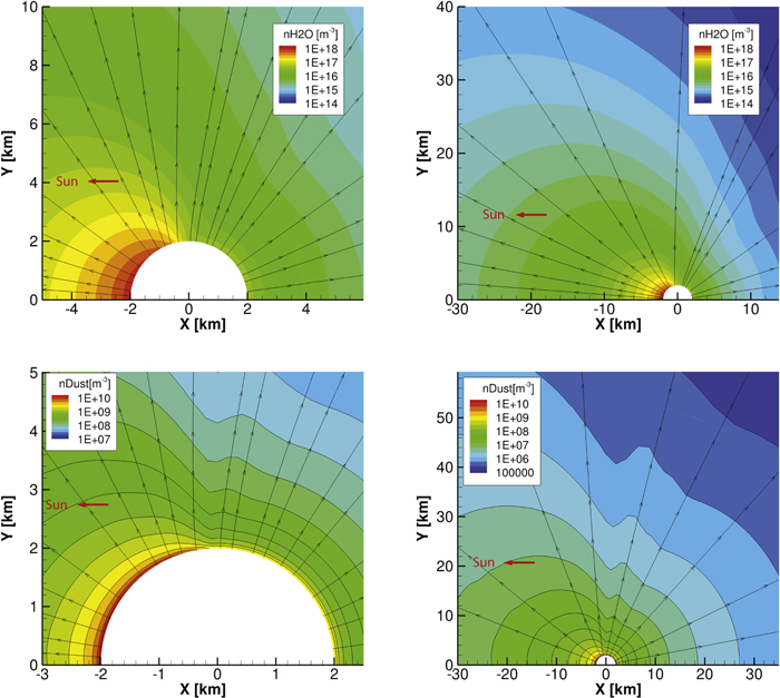
Figure 2. Number densities of H2O (upper panel) and all dust grains (lower panel) in the vicinity of the nucleus (left) and at a larger distance over 30 km (right) at a heliocentric distance of 1.3 au. The solid black lines are contour lines and the solid black lines with arrows are streamlines of H2O and dust velocities. The red arrow shows the directions of the Sun.
Download figure:
Standard image High-resolution imageFigure 3 offers an example of returning dust grains close to the comet. The results are similar to those in Figure 13 of Tenishev et al. (2011). Differences are due to the fluid nature of these calculations and the particle nature of the DSMC models. The Sun is in the negative x-axis direction. Near the terminator plane, the once lifted dust grains fall back to the nucleus. The dust speed on the nightside is comparable to that on the dayside, but the density of dust grains on the nightside is much lower than that on the dayside. We also want to point out that our returning dust grains are less abundant and travel a much shorter distance along the ground than those in the DSMC model. Our explanation is that the dust grains in the DMSC model can go in various directions at one point in space and those with a tangential velocity are more likely to return. In addition, the cells in the DSMC model are much smaller than the fluid model near the surface. With individual dust particles there are more opportunities for small scale structures in the DSMC. However, in the fluid model, all dust grains of the same size are treated as one fluid and share a single bulk velocity in the same computational cell. In our case, most of the lifted dust grains only have a radial velocity, which makes it difficult for them to return to the nucleus.

Figure 3. Number density and speed of the dust grains with a radius of 10−4 m near the nucleus at a heliocentric distance of 2.7 au from the fluid model results. The red arrow shows the directions of the Sun.
Download figure:
Standard image High-resolution imageFigures 4–5 show the total dust number densities and the mean dust speeds extracted from radial lines at several SZAs. The left column represents our model results and the right column shows the DSMC model results reproduced from Tenishev et al. (2011). Because of the power-law distribution, the total dust number is dominated by the smallest sized dust particles. As the mean dust speed is weighted by the number density, the mean speed is closest to the speed of the dust of the smallest size. The four rows represent four cases at different heliocentric distances: 1.3, 2.0, 2.7, and 3.3 au, respectively. The total gas production rates for the four cases are 5 × 1027, 8 × 1026, 8 × 1025, and 1 × 1024 s−1. The dust-to-gas mass ratio is 0.8 for all cases. It should be noted that these numbers are not from observations, and are used for model comparisons.
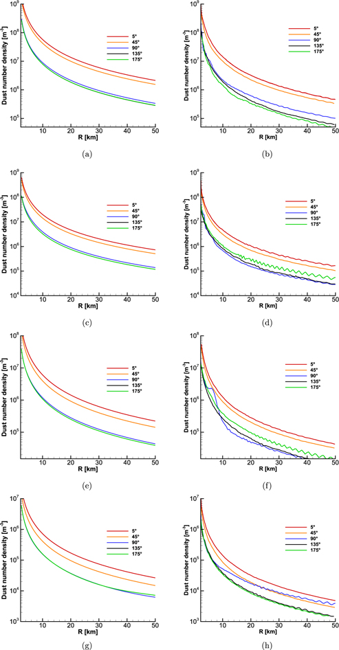
Figure 4. Dust number densities along radial lines at several subsolar angles as a function of cometocentric distance. The four rows represent four heliocentric distances of 1.3, 2.0, 2.7, and 3.3 au, respectively. The left column shows our model results and the right column is reproduced from Tenishev et al. (2011).
Download figure:
Standard image High-resolution image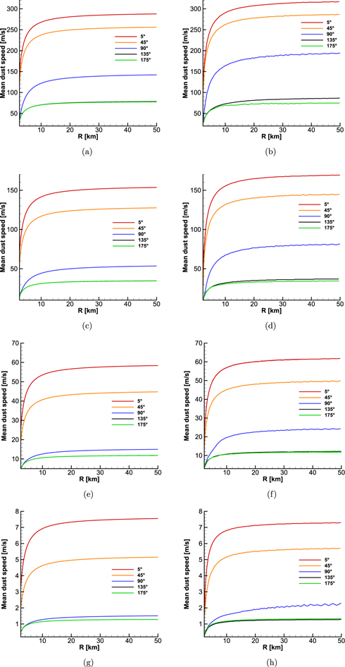
Figure 5. Mean dust speeds along radial lines at several subsolar angles as a function of cometocentric distance. The four rows represent four heliocentric distances of 1.3, 2.0, 2.7, and 3.3 au, respectively. The left column shows our model results and the right column is reproduced from Tenishev et al. (2011).
Download figure:
Standard image High-resolution imageIn Figure 4, two columns show similar trends: densities drop more sharply within 20 km than beyond that distance; lines at a lower SZA tend to have a larger density. We also note that the dust number densities in our model are about 2 ∼ 3 times those in the DSMC model. The major reason for the difference is the number of bins used to group dust grains by the radius. Since the dust number density distribution follows the power law with an index of −3, i.e.,  , the lower end of the spectrum has a higher number density. If the same amounts of dust mass are distributed into different bins of sizes by the same power law and dust velocities are the same, each bin should have the same amount of mass, since the mass of the dust grain
  and the mass density distribution is not dependent on size,
  . Therefore, if the same amount of mass is distributed in fewer bins, the smaller bins receive more mass. For example, in the case of 6 bins, the 10−7 m-sized grains have 1/6 of the total mass. Using the distribution function and increasing the number of logarithmically spaced discrete dust sizes to 40, now the 1/6 of the total mass will be distributed among bins of sizes ranging from 10−7 to
  m. As a result, the same amount of mass creates fewer dust grains in the case of 40 bins than in the case of 6 bins. Our model has 6 logarithmically spaced discrete dust sizes, while the DSMC model has about 50 bins and has a continuous distribution of sizes within each bin rather than 1 size per bin. Following the reasoning above, we expect our model with fewer bins to yield a higher total number density. One can also find that in the left column, the number density at the SZA of 90° is higher than that at 135° and 175° in almost all cases, while most cases in the right column do not show the same pattern. It may be caused by the dust grains, which are ejected at the lower SZA region but fall back to the surface at the higher SZA region.
Figure 5 shows the number density weighted average of the speed. The speeds in all plots increase sharply within 20 km, before reaching their terminal speeds. Similar to the behavior in the density plots, the speeds at lower SZAs are higher than those at larger angles, which is a result of higher gas flux and higher gas speed at lower SZAs and the almost radial expansion of the dust grains and gas. In the fluid model, the speeds at the SZAs of 135° and 175° are very close, while the DSMC model has a higher speed at 135°, which may indicate a more diffusive coma in the DSMC model, consistent with observations in other model comparison papers (Bieler et al. 2015). In addition, there are probably more odd particles coming from various original locations in the DSMC returning onto the nightside in different orientations, compared with the fluid model. We also note that the terminal speeds in the DSMC model are about 10% higher in most cases. This is likely caused by the dust grain's drag effect on H2O, which is included in our model but not in Tenishev et al. (2011). The ratio of gas kinetic energy to dust kinetic energy is also calculated for all the four cases. Generally, the ratio increases as the heliocentric distance gets larger, which is a result of lower dust terminal velocity and fewer liftable dust grains. The smallest ratio is about 9, which takes place on the dayside of the comet in the 1.3 au case, where most of the dust particles reach the terminal velocity. The largest ratio is more than 20,000, which is at the nightside in the 3.3 au case where most dust particles cannot be lifted.
Figures 6–7 show number densities and speeds of differently sized dust grains at a distance of 30 km to the nucleus as a function of the SZA. Similar to the previous figures, the left column represents our model results and the results in the right column are from the DSMC model. The four rows represent four cases at four heliocentric distances: 1.3, 2.0, 2.7, and 3.3 au, respectively. The expected difference in the dust number densities of neighboring sizes is about 3 orders of magnitude, according to the number distribution at the surface. Because of the difference in the velocities, the results have a difference in the number dust densities of neighboring sizes smaller than the expected value, indicating the number distribution in space is flatter than that at the boundary. In addition, both models display the classical dust speed's dependence on size,  . If one group of dust grains has a size 10 times larger than another group, the dust speed of the larger dust grains is about 1/3 of the smaller ones' speed.
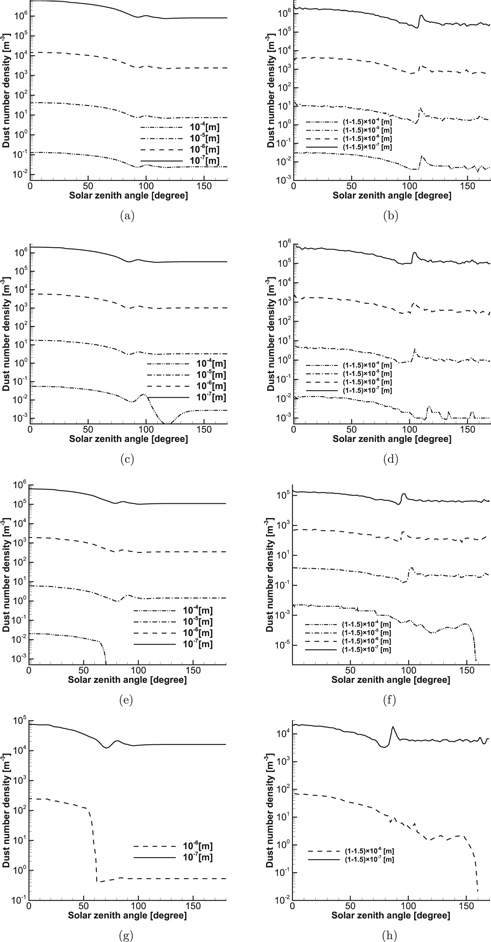
Figure 6. Dust number densities at a cometocentric distance of 30 km as a function of the solar zenith angle. The four rows represent four heliocentric distances of 1.3, 2.0, 2.7, and 3.3 au, respectively. The left column shows our model results and the right column is reproduced from Tenishev et al. (2011).
Download figure:
Standard image High-resolution image
Figure 7. Dust speed at a cometocentric distance of 30 km as a function of the solar zenith angle. The four rows represent four heliocentric distances of 1.3, 2.0, 2.7, and 3.3 au, respectively. The left column shows our model results and the right column is reproduced from Tenishev et al. (2011).
Download figure:
Standard image High-resolution imageFrom Figures 6–7, we can see that both models have quite similar profiles of dust densities and speeds, which in general have higher values at higher SZAs. Local maxima or spikes, corresponding to the spikes in the previous 2D plot, are also spotted in the line plots of the dust number densities from both models. The spikes in our model occur at a slightly lower SZA and appear less prominent than those in the DSMC model. For the dust grains that can be lifted, the variations in densities and speeds at different SZAs are smaller by one order of magnitude. Some large dust grains cannot be lifted on the nucleus surface beyond certain critical SZA, because their sizes exceed the local maximum liftable size. As a result of the boundary conditions, the densities and speeds of the large-sized dust grains are much lower beyond that critical SZA. The plots also show that at 30 km from the comet, such critical SZAs exist in both model results as well. For example, in the 2.7 au case, the critical SZA for 10−4 m dust grains at the inner boundary is about 70°. Our fluid model shows that at 30 km from the comet, the density and speed of 10−4 m-sized dust grains appear to be cut off beyond 70°, while in the DSMC model, the cutoff occurs near 150°, with a less abrupt change in the speed profile. The difference is likely to be caused by the limitation of the fluid model in treating the returning dust grains, as we discussed before. The observation above indicates once again that the dust grains in the DSMC model are more diffusive than those in our model, which we already mentioned in the previous discussion.
4.2. The Effects of the Cometary Activity and Rotation
This section studies the effects of the cometary activity and rotation on the dust grain's behavior. Figure 8 shows the densities of  and
and  dust at T = 24.8 hr under the different conditions of Case 1 (left) and Case 2 (right). We also want to restate here that in Case 1 the subsolar point is fixed on the big end of the nucleus, while in Case 2 the Sun is rotating around the nucleus with a period of 12.4 hr in the comet's reference frame. For Case 1, the subsolar longitude and latitude are 157° and −34°. For Case 2, the subsolar latitude is about −34°. The production rate and temperature used for these two cases are close to the 1.3 au case in Tenishev et al. (2011), but are also modified with the activity map from Fougere et al. (2016). In this section, a dust-to-gas mass ratio of 4 is used (Rotundi et al. 2015). We want to point out that this section is more of a theoretical study. The parameters used in the simulation may not be the same as those in the observations.

Figure 8. Number densities of dust grains with radii of 10−6 m (upper panel) and 10−3 m (lower panel) from Case 1 (left) and Case 2 (right) at T = 24.8 hr. For Case 2, the subsolar point is fixed on the nucleus. The red arrows point to the direction of the Sun.
Download figure:
Standard image High-resolution imageIn Figure 8 we can find that the density of  -sized dust grain shows a clear spiral pattern. In contrast, light and fast
  -sized dust grains are not affected significantly by the cometary rotation, because their speed is much larger than the co-rotating speed of about 5 m s−1 at a distance of 40 km. Since 24.8 hr are about two rotation periods, the subsolar points for two cases are at the same location. In addition, because of the high speeds of smaller particles, the density profiles of
  -sized dust grains are not affected much by the dust particles emitted before. As a result,
  -sized dust grains show similar density distributions in both cases. We can also see that the spiral pattern in Case 1 is much more prominent than that in Case 2. Case 2 has more spirals and more uniformly distributed dust grains. These results may suggest that if there is one dominant jet or activity independent of the solar illumination, a clear spiral pattern has a high probability of existing in the plane perpendicular to the rotating axis. The combination of the solar illumination and the nucleus rotation is also able to produce spirals, which may be more difficult to observe.
Figure 9 shows the speeds of differently sized dust grains at distances of 30 km (left) and 50 km (right) at the z = 0 plane, from Case 2 as a function of the azimuthal angle ϕ. The azimuthal angle ϕ starts from 0 in the direction of x-axis and increases clockwise. We find the 10−5 m-sized dust grains are consistently faster than the other two groups. Due to the effect from the cometary activity and rotation, the speeds of 10−3 m-sized and 10−4 m-sized dust grains are small and close to each other. They do not reveal a clear dependence on size, especially at 50 km from the nucleus, which is different from the model results in Section 4.1. Without rotation and cometary activity, the speeds of smaller dust grains are strictly higher than the larger ones. A similar conclusion is also reached by dust measurements (Rotundi et al. 2015). Measurements in the coma of comet 67P were performed by the impact sensor (IS) and the grain detection system (GDS) of GIADA. The GDS is able to detect dust grains when they pass through a laser curtain near the spacecraft, while the momentum of dust grains is measured by the IS. GDS alone provides the speeds and optical cross sections of grains. When it is combined with the IS momentum measurements, the mass density of the dust grains can be more accurately characterized than it could be with one instrument. The measured dust grains have sizes within  and
and  and most of them are detected at cometocentric distances between 30 and 50 km. Our model may suggest that rotation and the heterogeneity of activity are one interpretation as to why there is no clear dust speed dependence on size, as shown by the GIADA observations (Rotundi et al. 2015).
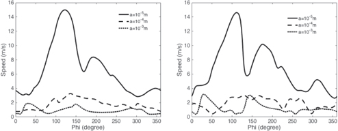
Figure 9. Speeds of 10−3–10−5 m-sized dust grains at cometocentric distances of 30 km (left) and 50 km (right) at z = 0 plane from Case 2. The x-axis is the azimuthal angle ϕ, which starts from 0 in the direction of the x-axis and increases clockwise.
Download figure:
Standard image High-resolution image4.3. Comparison with Dust Observations
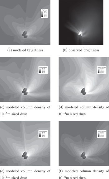
In this section, we will compare our model results with the images obtained by OSIRIS/WAC on 2015 May 30. Figure 10 shows the time series of dust brightnesses derived from our time-dependent runs and from the observations. The modeled brightness is calculated by the dust column densities times the product of the geometrical cross sections and the scattering efficiency. Since the scattering efficiency for 10−7 m-sized particles is extremely low, the brightness calculation does not account for the contribution from 10−7 m-sized particles. According to Fink & Rubin (2012), given a fixed phase angle, the difference in the white light scattering efficiencies of differently sized dust particles is lower than a factor of 3. For simplicity, we assume the scattering efficiency for particles with sizes ranging from 1 μm to 1 cm are the same. The OSIRIS/WAC images are obtained from the NASA PDS Small Bodies Node and more details about the instrument can be found in Keller et al. (2007). We can see in Figure 10 that our model results can capture most of the large-scale distributions of observed dust brightness. The images at 18:43 May 30, do not match very well, the discrepancy potentially due to localized and temporary activities on the nucleus surface.

Figure 10. Comparison of the dust brightness derived from the model (left) and from the observations (right). Different rows represent brightness modeled and observed at different times on 2015 May 30. The images from the right column are originally obtained from the data set "Gutierrez-Marques, P., Sierks, H. and the OSIRIS Team, ROSETTA-ORBITER COMET ESCORT OSIWAC 3 RDR MTP 016 V1.0, RO-C-OSIWAC-3-ESC2-67PCHURYUMOV-M16-V1.0, ESA Planetary Science Archive and NASA Planetary Data System, 2016" and are adjusted to log scale.
Download figure:
Standard image High-resolution imageFigure 11 shows the dust column densities of different sizes. We can see the images of 10−4 and 10−5 m are most similar to the modeled and observed brightness, which suggest these sized particles play an important role in the dust white light brightness. The 10−4 and 10−5 m-sized dust particles resemble the observed image more than the smaller ones in terms of the overall structure and some fine features. For example, similar curved jets can be found in the 10−4 m-sized dust column density and the OSIRIS/WAC image. However, the jet in our model result is larger than observed. It may imply the curved jet is composed of even larger particles. It is also possible that the modeled jet originates from a broader activity region in the model than in the real world, because the gas surface activity distribution obtained from the ROSINA measurements (Fougere et al. 2016), is inherently rather coarser than the dust distribution. While it is sufficient to reproduce the gas observations and the larger-scale features of the dust, a more refined activity distribution is required to get the very fine structure. Nevertheless, the agreement between our model and the observations shows that the OSIRIS/WAC image is a better proxy for the column densities and brightness of dust of size from 10−4 and 10−5 m, and the curved jet mainly consists of larger dust particles, which is also suggested by Lin et al. (2016).
Figure 11. Comparison of modeled column densities of different sizes and observed and modeled dust brightness on 15:13:39 UT, 2015 May 30.
Download figure:
Standard image High-resolution image
As we discussed earlier in Section 4.1, smaller dust particles have higher speeds. Once the boundary condition changes, the density profiles of small dust particles are refreshed quickly by the newly born particles from the nucleus. Large dust particles can remain close to the nucleus for quite a long time, thus snapshots of dust brightness and column density contain the history of previous illumination conditions. As a result, a time-dependent model is better equipped to account for the history information, which is essential to interpret some features in dust images.
5. Summary
In this work, we have developed a new 3D cometary dust model that takes into account the major physical processes governing the dust–gas interaction, and applied the multi-fluid dust model to comet 67P/Churyumov–Gerasimenko. Our model is compared with a DSMC model, which has been successfully applied to study various cometary problems. The comparison shows good agreement, and also illustrates the limitations of the fluid approach in modeling the returning dust grains. In order to study the effects of the cometary activity and rotation, time-dependent simulations are run on a newly developed "roundcube" mesh in the rotating cometary reference frame, with necessary fictitious forces. Our results reveal that a spiral pattern can be found for heavy and large dust grains. If a dominant jet persists on the comet, the spiral can be more prominent. In addition, the effect of rotation offers one explanation to the question why there is no clear dust speed dependence on size in some of the dust observations performed by Rosetta/GIADA. A comparison between the model results and the observed dust images suggests 10−4 and 10−5 m-sized dust particles are important to understand some features of the Rosetta OSIRIS/WAC images, and also those features can only be interpreted by a time-dependent model. As illustrated by the results shown in this paper, our new multi-fluid dust model is capable of solving complex and time-dependent problems, and therefore holds a promising future for applications to understanding complex gas–dust interactions in other planetary and astrophysical systems.
The work at the University of Michigan was supported by NASA Planetary Atmospheres grant NNX14AG84G, and contracts JPL#1266314 and JPL#1266313 from the U.S. Rosetta project. Resources for all simulations in this work have been provided by NASA High-End Computing Capability (HECC) project at NASA Advanced Supercomputing (NAS) Division.