


Abstract
This paper reports a reanalysis of archival ALMA data of the high velocity(-width) compact cloud CO−0.40–0.22, which has recently been hypothesized to host an intermediate-mass black hole (IMBH). If beam-smearing effects, difference in beam sizes among frequency bands, and Doppler shift due to the motion of the Earth are considered accurately, none of the features reported as evidence for an IMBH in previous studies are confirmed in the reanalyzed ALMA images. Instead, through analysis of the position–velocity structure of the HCN J = 3–2 data cube, we have found kinematics typical of a cloud–cloud collision (CCC), namely, two distinct velocity components bridged by broad emission features with elevated temperatures and/or densities. One velocity component has a straight filamentary shape with approximately constant centroid velocities along its length but with a steep, V-shaped velocity gradient across its width. This contradicts the IMBH scenario but is consistent with a collision between two dissimilar-sized clouds. From a non-LTE analysis of the multitransition methanol lines, the volume density of the post-shock gas has been measured to be ≳106 cm−3, indicating that the CCC shock can compress gas in a short timescale to densities typical of star-forming regions. Evidence for star formation has not been found, possibly because the cloud is in an early phase of CCC-triggered star formation or because the collision is nonproductive.
Export citation and abstract BibTeX RIS
1. Introduction
High velocity(-width) compact clouds (HVCCs) are a population of dense gas clumps with peculiarly broad-lined molecular emissions having full width at zero intensity (FWZI) width of a few tens to 100 km s−1 (Oka et al. 2012; Tanaka et al. 2015). Approximately 100 HVCCs and similar broad molecular-line features have been identified in the central molecular zone (CMZ) in the Galaxy (Oka et al. 2012; Tokuyama et al. 2017). They are approximately a factor of 5 above the standard size–linewidth relation for the CMZ clouds, indicating the ubiquitous presence of energy-injecting events in the CMZ. Supernova (SN)–cloud interactions (Tanaka et al. 2009; Yalinewich & Beniamini 2017) and cloud–cloud collisions (CCCs; Tanaka et al. 2015; Ravi et al. 2017) have been proposed as candidates for these energy sources.
Recently, following a series of observational studies, Oka et al. (2016, 2017) have proposed a new hypothesis for the formation of the archetypical HVCC CO−0.40–0.22 (hereafter, CO−0.4): gravitational acceleration by an intermediate-mass black hole (IMBH). The cloud CO−0.4 is one of the most energetic HVCCs, which have 90 km s−1 wide HCN and SiO emissions (Tanaka et al. 2015; Oka et al. 2016). Oka et al. (2016) have interpreted this broad-lined molecular emission as a high velocity gas stream trailing from a clump that was kicked by the gravitational interaction with an IMBH of 105 M⊙. Although the spatial-velocity structure of the cloud was not fully resolved in their original single-dish images, a follow-up interferometric study using the Atacama Large Millimeter–submillimeter Array (ALMA) has identified a clump with extremely broad-lined emission, 110 km s−1 wide FWZI, at the position of the gravitationally kicked clump predicted by their model (Oka et al. 2017). In addition, they claim that a point-like continuum source near the clump, CO−0.4*, is self-absorbed synchrotron emission from an IMBH, based on the shallow spectral index α = 1.18 ± 0.65 measured in the 230–265 GHz frequency range.
This "gravitational-kick" formation scenario seems to successfully explain the cloud kinematics, but it should be noted that the model is based on single-dish images with insufficient resolution. Although a candidate for the gravitationally kicked clump has been identified in the high-resolution ALMA images, a direct comparison between the gas stream model and the position–velocity (PV) structure of the high-resolution ALMA image has yet to be performed. In addition, the significance of the nonthermal spectral energy distribution (SED) ascribed to the IMBH candidate has been called into question by a recent follow-up study. Ravi et al. (2017) reported a nondetection of CO−0.4* at 34.25 GHz, which is contradictory to the shallow value of α obtained from the ALMA data and instead indicates thermal emission from warm dust. Furthermore, it is not clear whether such exotic objects as IMBHs could create the HVCCs which are commonly found in the CMZ, as questioned by Yalinewich & Beniamini (2017); these authors argue that the sum of the cloud mass and IMBH mass must be greater than the total mass of the CMZ in order to explain the observed HVCC formation rate with the IMBH scenario.
In the present paper, we re-examine the gravitational-kick scenario by analyzing the same ALMA data used in Oka et al. (2017). We find no evidence for gravitational interaction with an IMBH in the reanalyzed ALMA data, when beam-smearing effect and time variation of the Doppler-shifted frequencies due to the motion of the Earth are considered accurately. We investigate a CCC hypothesis as an alternative for the origin of the broad-lined molecular emission from CO−0.4.
2. Reanalysis of the ALMA Archival Data
We reanalyzed the ALMA data used by Oka et al. (2017), which we obtained from the ALMA science archive (id: 2012.1.00940.S). The data include multiple data sets observed with different antenna-array configurations from 2013 July to 2015 January. Table 1 summarizes information about the data sets, with the observations labeled by the execution dates. The spectral data were taken in three frequency windows centered at 230 GHz, 250 GHz, and 265 GHz. The 250 and 265 GHz data were obtained simultaneously. The 230 and 265 GHz bands have an ∼900 MHz bandwidth and a ∼200 kHz channel separation, and are observed with both the 12 m and 7 m arrays. The 250 GHz data were taken with a broadband mode with a ∼2 GHz bandwidth and a 15 MHz channel width, and lack 7 m array data.
Table 1. ALMA Data
| Data seta | Array | Band | Calibratorsb | uvc |
|---|---|---|---|---|
| GHz | Flux/Bandpass/Gain | kλ | ||
| 07OCT2013 | 7 m | 230 | Nep./J1924/J1744 | 7–37.5 |
| 01NOV2013 | 7 m | 230 | Nep./J1924/J1744 | 5.5–37.5 |
| 22JAN2015 | 12 m | 230 | Titan/J1517/J1744 | 10–252 |
| 13APR2014 | 7 m | 265 | Mar./J1427/J1744 | 7–42 |
| 29DEC2014 | 7 m | 265 | Titan/J1733/J1744 | 8.5–40 |
| 08JUL2013d | 12 m | 250,265 | J2232/J2258/J2337 | 10–390 |
| 11MAR2014 | 12 m | 250,265 | Titan/J1517/J1745 | 11.5–332 |
Notes.
aNamed according to the execution dates; 07OCT2013 was obtained on 2013 October 7, and so on. bAbbreviations for the calibrator source names: Nep. = Neptune, Mar. = Mars, J1924 = J1924-2924, J1744 = J1744-3116, J1517 = J1517-2422, J1427 = J1427-4206, J1733 = J1733-1304, J2322 = J2322+117, J2258 = J2258-2758, J2337 = J2337-230, J1745 = J1745-290. cValues after flagging. dLacks correct Tsys calibration. Not used in the final images.Download table as: ASCIITypeset image
We employed standard data reduction procedures, using the Common Astronomy Software Applications (CASA) package developed by the National Radio Astronomy Observatory (NRAO); flagging low quality data, correction for atmospheric conditions, and calibration of the visibility data were performed using the reduction script provided by the ALMA observatory. The calibrators used for bandpass, flux, and complex gain calibrations are listed in Table 1. The 08JUL2013 data lacks calibration data for the system noise temperature for multiple antennas; therefore, for this data set, we substituted the averaged values for the other antennas.
The main target lines are CO J = 2–1 (230.538 GHz) and HCN J = 3–2 (265.886 GHz). We also detected more than 20 other lines, which are listed in Table 2, in the three spectral windows. The spectra in the 230 and 265 GHz bands are separated into line and continuum components using the UVCONTSUB task in the CASA package. Continuum subtraction was not possible for the 250 GHz band data due to the extreme crowdedness of the emission lines.
Table 2. Detected Lines
| Molecule | Transition | Frequency | Notes |
|---|---|---|---|
| (GHz) | |||
| CH3OH | 3−2–4−1E | 230.027 | |
| CO | 2–1 | 230.538 | |
| CH2NH | 71,6–70,7 | 250.162 | |
| CH3OH | 133,10–132,11A−+ | 250.291 | |
| NO | 5/2–3/2 | 250.44 | |
| 250.45 | |||
| CH3OH | 110,11–101,10A++ | 250.507 | |
| NO | 5/2–3/2 | 250.708 | |
| 250.816 | |||
| CH3OH | 123,9–122,10A−+ | 250.635 | |
| 113,8–112,9A−+ | 250.924 | ||
| SO2 | 131,13–120,12 | 251.200 | blended |
| 83,5–82,6 | 251.211 | ||
| c-HCCCH | 62,5–51,4 | 251.314 | |
| CH3OH | 93,6–92,7A−+ | 251.360 | |
| CH2NH | 60,6–51,5 | 251.421 | |
| CH3OH | 83,5–82,6A−+ | 251.517 | blended |
| c-HCCCH | 71,7–60,6 | 251.527 | |
| t-CH3CH2OH | 151,15–140,14 | 251.567 | |
| CH3OH | 73,4–72,5A−+ | 251.642 | |
| 63,3–62,4A−+ | 251.739 | ||
| 53,2–52,3A−+ | 251.812 | ||
| CH2NH | 41,3–31,2 | 266.270 | |
| HCN | 3–2 | 265.886 |
Download table as: ASCIITypeset image
We performed mosaic imaging using the TCLEAN task. Briggs weighting with a robustness parameter of 1 was applied for the 230 GHz band line data, and the natural weighting was applied for the 250 and 265 GHz line data. For the continuum maps, robustness of 1 and a uv-taper at the 1'' angular scale were applied for the 230 GHz and 265 GHz data, respectively, to improve the signal-to-noise ratio. The synthesized beam sizes and beam position angles are listed in Table 3. The 250 and 265 GHz maps have smaller beam widths than the 230 GHz maps, as the former were obtained with more extended antenna configurations. We refined the image quality by performing self-calibration cycles using the moment-0 CO and HCN images independently for each data set. We excluded the 08JUL2013 data from the final imaging, since the moment-0 map constructed from this data was inconsistent with the images from other 265 GHz band data, presumably due to incorrect calibration and the lack of correct Tsys measurement data.
Table 3. Image Data
| Band | Line/Continuum | Array | bmaj × bmin | Beam P.A. |
|---|---|---|---|---|
| GHz | arcsec2 | deg. | ||
| 230 | continuum | 12 m + 7 m | 2.03 × 1.24 | 74.6 |
| 265 | continuum | 12 m + 7 m | 1.98 × 1.35 | 71.9 |
| 230 | line | 12 m + 7 m | 1.75 × 1.02 | 74.9 |
| 265 | line | 12 m + 7 m | 1.35 × 0.60 | 69.8 |
| 250 | line+continuum | 12 m | 1.42 × 0.59 | 69.9 |
Download table as: ASCIITypeset image
3. Results
3.1. The −80 km s−1 Filament and Knots
Figure 1 shows the integrated intensity maps and the PV diagrams for the HCN J = 3–2 and CO J = 3–2 lines. The PV diagrams are plotted along the right ascension (R.A.) axis and are averaged over the full decl. range. Multiple velocity components exist along the line of sight toward the target cloud. The emission from CO−0.4 extends from −110 to −20 km s−1 in the velocity of the local standard of rest (LSR) (vLSR). The 13CO J = 2–1 image is self-absorbed at vLSR = −50, −25, and −5 km s−1 by foreground clouds in the Galactic disk, whereas the HCN J = 3–2 data are almost free of self-absorption dips for the velocity range of CO−0.4. The narrow line emission at vLSR = 20 km s−1 in the CO J = 2–1 PV diagram is the foreground infrared dark cloud G359.62−0.24 (or the "Freccia Rossa" cloud; Bally et al. 2010; Ravi et al. 2017), which is seen as an absorption dip in the HCN J = 3–2 image. Other positive-velocity emissions are from Galactic center (GC) clouds unrelated to CO−0.4.

Figure 1. (Top panels) HCN J = 3–2 and CO J = 2–1 flux densities integrated over the velocity range −110–0 km s−1. (Bottom panels) Position–velocity diagrams for HCN J = 3–2 and CO J = 2–1 projected on the right ascension (R.A.) axis, averaged over the full declination (decl.) range. The emission from the CO−0.4 exists primarily in the velocity range of −110 to −10 km s−1. Clouds with positive velocities are the foreground cloud G359.62−0.24 or Galactic center clouds unrelated to CO−0.4.
Download figure:
Standard image High-resolution imageThe CO integrated intensity map illustrates the highly complicated cloud structure, which consists of many small, entangled filamentary features. In contrast, most of the spatially extended emissions are transparent in the HCN J = 3–2 image, in which the central high-density portion of the cloud is captured owing to its high critical density (ncrit). In Section 3.2., we mainly use the HCN J = 3–2 data to analyze the cloud structure.
Figure 2 shows the continuum maps at 230 and 265 GHz. We identified two bright point-like sources that are present in both frequency bands, which we labeled MM1 and MM2. Source MM1 corresponds to the IMBH candidate CO−0.4* (Oka et al. 2017); it is not an isolated point source in our images, but is located in a ridge-like extended background emission 7'' long.

Figure 2. Continuum maps of the 230 and 265 GHz bands. Positions of the two bright point-like sources, MM1 and MM2, are indicated by cross marks.
Download figure:
Standard image High-resolution imageFigure 3 shows the spectra of the three spectral windows averaged over the five positions indicated in Figure 4. In addition to the CO and HCN lines, more than 20 lines from CH3OH, CH2NH, NO,  , and c-HCCCH are detected. These emissions are mostly concentrated in a filament running through the central region of CO−0.4 in an approximately southeast–northwest direction, as represented by the CH3OH 110–101 map shown in Figure 4. This filament has an approximately constant velocity of approximately −80 km s−1 throughout the full length. A corresponding filamentary structure is also seen in the HCN map in the −90 to −70 km s−1 velocity range. We refer to this structure henceforth as the −80 km s−1 filament. The brightness of the filament in optically thin methanol and other rare molecular lines indicates that the filament is the densest part of CO−0.4.

Figure 3. Spectra of the 230, 250, and 265 GHz bands averaged over the five intensity peaks indicated in Figure 4. The 230 and 265 GHz spectra are averaged over every 32 channels.
Download figure:
Standard image High-resolution image
Figure 4. Peak-intensity maps for HCN J = 3–2 (left) and CH3OH 110–101 A++ (right), calculated from data smoothed into 2 km s−1 and 36 km s−1 velocity bins, respectively. The HCN J = 3–2 intensities are measured for the velocity range −100 to −70 km s−1. The shape of the −80 km s−1 filament is indicated in the HCN map, with two prominent features, labeled knot-A and knot-B. The crosses on the CH3OH map are the positions of the averaged spectra used in Figure 2 and the population diagram analysis (Section 3.3). An approximate shape for the hypothesized gas stream (read from Figure 3 of Oka et al. 2016) is indicated by the dashed lines.
Download figure:
Standard image High-resolution imageThe −80 km s−1 filament has a few knots with bright methanol emissions. The two brightest knots are labeled as knots A and B in Figure 2. Both knots are also bright in the HCN J = 3–2 image, and the filament is wider at knot B than at other portions along its length. Knot B is located at the position where Oka et al. (2017) reported the gravitationally kicked cloud.
3.2. The Cloud Structure and Velocity Field
3.2.1. Three Velocity Components
In this section, we analyze the internal structure and velocity field of CO−0.4 using the HCN J = 3–2 data cube. First, we extract the primary structure of the cloud in position–position–velocity (PPV) space by means of the dendrogram method (Rosolowsky et al. 2008); this step is necessary since the HCN data cube exhibits highly complicated PPV structure, in which almost every line-of-sight contains multiple velocity components including those physically unrelated to the main body of the cloud. We identified six main branches in the dendrogram created from the HCN data cube, and reconstructed the image of the primary PPV structure by pruning other minor structures and components unrelated to the cloud. The details of the dendrogram analysis are described in the Appendix.
Figure 5 shows the averaged spectra for the six main branches. The figure indicates that the cloud consists of three major velocity components: two narrow line components at −40 and −80 km s−1, and a moderately broad component at −60 km s−1. The FWZI velocity widths are 10 km s−1 for the −40 and −80 km s−1 components, and 50 km s−1 for the −60 km s−1 component. The single-dish HCN J = 4–3 spectrum averaged over the entire cloud (Tanaka et al. 2014) is also presented in the figure for comparison, showing that the broad profile of the averaged spectrum is the superposition of the three velocity components at −40, −60, and −80 km s−1, with ≲50 km s−1 widths, but none of the six main branches alone can account for the ∼90 km s−1 velocity width of the averaged spectrum.

Figure 5. Spatially averaged HCN J = 3–2 spectra of the main branches, which are normalized so that the peak intensities are unity. The top spectrum is the HCN J = 4–3 spectrum obtained with the ASTE 10 m telescope (Tanaka et al. 2014), averaged over the entire cloud.
Download figure:
Standard image High-resolution image3.2.2. Moderately Broad-line Emissions
Figure 6 shows the 2D maps of the zeroth moment, first moment (moment-0 and moment-1), and velocity width (Δv), which are created from the reconstructed image of the main structure of the cloud. The quantity Δv is defined by the moment-0 values divided by the spectral-peak flux densities pixel-by-pixel. We also show the moment-1 map of the HCN map smoothed to a 20'' resolution, i.e., the typical resolution of the previous single-dish observations (Tanaka et al. 2014; Oka et al. 2016) in Figure 6(d).

Figure 6. Maps of (a) moment-0, (b) moment-1, (c) velocity widths (Δv), and (d) moment-1 smoothed with 20'' Gaussian for the cloud image reconstructed from the six main branches and their common trunk nodes. The width Δv is defined as the moment-1 value divided by the spectral-peak intensity toward each line of sight. The 2D spatial distributions of the branches are shown by the contours overlaid on the moment-0 map. The shape of the −80 km s−1 is denoted by the dashed-lined curves on the moment-1 and Δv maps, which are identical to that in Figure 4. The rectangles in the moment-1 map indicate the strips for the PV diagrams in Figures 8 and 11. The approximate shape of the hypothesized gas stream (Oka et al. 2016) is shown in panel (d).
Download figure:
Standard image High-resolution imageThe Δv map (Figure 6(c)) shows that individual spectra consisting of CO−0.4 are predominantly narrow; approximately 75% of the pixels have Δv narrower than 15 km s−1, and the most frequent value is 10 km s−1. These velocity widths are smaller than the variation in the moment-1 velocities over the entire cloud, ∼60 km s−1. Pixels with Δv larger than 25 km s−1 are 5% of the entire map, and their spatial distribution is concentrated to a few narrow areas near the −80 km s−1 filament, in particular, to knots A and B. This confirms that the 90 km s−1 width broad emission in the single-dish image consists of a superposition of multiple velocity components with narrow velocity widths.
Figure 7 is a close-up view of knots A and B that presents the distributions of the three velocity components and the moderately broad emission with Δv > 25 km s−1. The figure shows that the −40 and −80 km s−1 components are loosely anti-correlated with each other on the plane of the sky. In addition, the spatial distribution of the −60 km s−1 component is correlated well with that of the moderately broad emission, and both extend along the narrow boundary regions between the −80 and −40 km s−1 components. This indicates that the moderately broad emissions and the −60 km s−1 component are the same physical entity, and they represent the transition region of the other two components in PPV space; this structure can be interpreted such that the line-broadening at knots A and B is caused by a physical interaction between −80 and −40 km s−1 components.

Figure 7. (Left panel) Composite color image of the HCN J = 3–2 flux densities averaged over the velocity ranges [−30 km s−1, −50 km s−1] and [−90 km s−1, −70 km s−1] (in red and cyan, respectively) near knots A and B, with overlaid contours of Δv at levels of 25, 30, 35, and 40 km s−1. (Right panel) Map of the HCN J = 3–2 flux density averaged over the velocity range [−70 km s−1, −50 km s−1], with the same contours of Δv as those in the left panel. The spatial distribution of the broad emission with Δv ≥ 25 km s−1 is correlated well with the −60 km s−1 component, and appear almost exclusively in the boundary regions between the −80 and −40 km s−1 components.
Download figure:
Standard image High-resolution image3.2.3. V-shaped Velocity Gradient across the −80 km s−1 Filament
Figure 8 presents PV diagrams of the original HCN J = 3–2 data for two cuts crossing the −80 km s−1 filament at the locations of knots A and B. Along both cuts, the PV diagrams show characteristic V-shapes; the −80 km s−1 filament and the −40 km s−1 component are smoothly bridged by a pair of bright emission features with steep velocity gradients. These bridging emissions correspond to the moderately broad −60 km s−1 component identified with the dendrogram analysis. We note that this V-shape is not a PV pattern that appears only along these two particular cuts, but it persists over a wide spatial range along the filament. The moment-1 map (Figure 6(b)) shows that the northern part of the filament from knot A to knot B is interposed by a pair of bands with −60 to −40 km s−1 velocities that are running parallel to the filament; this configuration is observed as the V-shaped pattern across cuts perpendicular to the filament. Formation of this V-shaped PV pattern is readily explained by assuming physical interaction between the −80 km s−1 filament and clouds at −40 km s−1. We will discuss this in more detail in a later section (Section 4.2).

Figure 8. PV diagram of the original HCN J = 3–2 data along strips-A and -B across the −80 km s−1 filament. The strips are indicated by the rectangular regions in Figure 6(b), where the X axes are taken in the directions of the long sides of the rectangles. The spectra are averaged over the short sides. The V-shaped patterns indicative of cloud–cloud interaction are clearly recognizable.
Download figure:
Standard image High-resolution image3.3. Heating Sources inside or near the −80 km s−1 Filament
We have investigated the physical conditions in the −80 km s−1 filament by means of a population diagram. Figure 9(a) shows the rotational population diagrams for the a-CH3OH and CH2NH lines, constructed from the peak-intensity values of the spectra averaged over the five positions along the filament indicated in Figure 4. We ignored the c-HCCCH line that blended with the 251.517 GHz CH3OH line, assuming that the former is significantly weaker than the latter. The error bars include both the rms noise measured for a blank-sky region in the data cube and conservatively assumed 20% relative errors. The rate coefficients and partition functions are taken from the Leiden Atomic and Molecular Database (LAMDA; Schöier et al. 2005), the Cologne database for molecular spectroscopy (CDMA; Muller et al. 2001), and Motoki et al. (2014).

Figure 9. (a) Rotational population diagram for CH3OH and CH2NH in the −80 km s−1 filament. (b) Physical conditions in the filament calculated from a non-LTE analysis using the methanol lines. Credible intervals obtained from a flat-prior Bayesian analysis are shown by the colored contours.
Download figure:
Standard image High-resolution imageEach of the a-CH3OH and CH2NH level population diagrams is consistently fitted by a single-component, local thermodynamic equilibrium (LTE) curve except for the 250.507 GHz line of methanol, which is a predicted class-I maser line (Voronkov et al. 2012). The diagram indicates two temperature components, corresponding to cold gas with a CH2NH rotational temperature Trot ∼ 24 K and warm gas with a CH3OH rotational temperature Trot ∼ 70 K. Although accurate values of ncrit for the CH2NH lines are unknown, the similar A coefficients for the CH3OH and CH2NH lines (∼10−4 s−1) allow us to assume that they have similar values of ncrit and hence that the different Trot values reflect differences in the physical conditions of the emitting regions.
We performed a non-LTE analysis for the methanol lines using collisional excitation coefficients taken from LAMDA, where the gas kinetic temperature Tkin, column density N, and hydrogen volume density  , are taken as free parameters. Figure 9(b) shows the simultaneous credible intervals for Tkin and
  , calculated from a Bayesian analysis assuming a prior function that is flat for 1 < Tkin/K < 1000 and 1 <
  /cm−3 < 107 and zero otherwise. Although the degeneracy between Tkin and
  is not resolved, this result indicates that the filament has highly elevated Tkin and/or
  compared with the physical conditions of standard GC clouds, for which Tkin = 30–100 K and
  = 104 cm−3 (e.g., Martin et al. 2004; Nagai et al. 2007; Arai et al. 2016; Ginsburg et al. 2016). In particular, this analysis indicates that
  ≳ 106 cm−3, unless an unrealistically high Tkin of > 103 K is assumed. This result is also consistent with that from a non-LTE analysis using HCN lines (Tanaka et al. 2014).
It is worthwhile to note that Trot of 70 K for the warm component is among the highest of those measured for the CMZ clouds; it is comparable to that measured toward the Sgr B2 hot cores. In contrast, typical CMZ clouds have 10–20 K CH3OH rotational temperatures (Requena-Torres et al. 2006). The coexistence of this exceptionally high-temperature gas and the cold component indicates the existence of some heating mechanism working near or inside the −80 km s−1 filament.
The column densities of CH2NH and CH3OH obtained from the non-LTE analysis are not particularly large compared with those in typical GC clouds or hot cores. We calculated the fractional abundances of CH2NH and CH3OH to be 2 × 10⁻⁸ and 1 × 10⁻⁷, respectively, using hydrogen column densities obtained from the 265 GHz dust flux assuming a dust temperature of 20 K and dust-emissivity index of 1.5. These abundances are typical values for hot cores or GC clouds (Requena-Torres et al. 2006; Suzuki et al. 2016).
4. Discussion
4.1. Comparison with the Gravitational Kick Model
The observational bases of the gravitational-kick scenario presented by Oka et al. (2016, 2017) can be summarized as follows:
- 1.The low-resolution images obtained with the NRO 45 m and ASTE 10 m telescopes show a slightly elongated elliptical shape. Oka et al. (2016) detected a steep velocity gradient from −110 to −20 km s−1 across the major axis, and interpreted it as a beam-smeared image of a gas stream formed thorough IMBH–cloud interaction. Although the stream is not fully resolved in the single-dish images, which have ∼20'' angular resolutions, Oka et al. (2016) predicted its PV structure on the basis of numerical simulations.
- 2.Oka et al. (2017) identified a compact clump with an extremely broad emission of a 110 km s−1 width near the predicted position of the hypothesized IMBH, using the high-resolution image obtained with the ALMA observation. The authors consider that this extremely broad emission clump had been scattered by tidal interactions with the IMBH. The PV position of the clump is approximately consistent with the trajectory of the stream predicted by Oka et al. (2016).
- 3.Oka et al. (2017) argued that the compact continuum source MM1/CO−0.4* is self-absorbed synchrotron emission from an IMBH, on the basis of the shallow spectral index of α = 1.18 ± 0.65 measured from the continuum fluxes at 230 and 265 GHz. The position of the source is consistent with the locus of the gravitational source in the model in Oka et al. (2016).
In this section, we examine these arguments using our reanalyzed ALMA data.
4.1.1. Stream
First, we examine the significance of the steep velocity gradient detected in the single-dish images. The spatial width of the velocity gradient in Oka et al. (2016) is no greater than 2–3 times the resolution; in such under-resolved images, beam-smearing effects can create an artificial gradient wherever multiple velocity components overlap. In fact, the moment-1 map (Figure 6(b)) shows the absence of a large-scale, monotonic velocity gradient on the entire-cloud scale; instead, the velocity field is dominated by very steep variations on ∼5'' spatial scales created between the patches of −40 km s−1 emissions and the widespread −80 km s−1 emissions. This indicates that the streamer-like velocity structure reported in Oka et al. (2016) is nonphysical, but instead is a product of the severe beam-smearing effect on the multicomponent velocity field. We confirmed that the 20''-resolution moment-1 map (Figure 6(d)) exhibits an apparently smooth gradient that is consistent with that observed in the single-dish data.
Second, we examine the validity of the stream model directly by comparing it with the ALMA data. The approximate shape of the predicted stream is overlaid on the methanol map (Figure 4(b)). Obviously, a stream structure consistent with the model is not detected in any of the molecular or continuum images. The most conspicuous stream-like structure in our data is the −80 km s−1 filament, but its direction is perpendicular to that of the predicted stream. In addition, the filament lacks a systematic velocity gradient along its length that would be expected for a stream from a gravitationally kicked clump. The velocity gradient is steepest across the width of the filament, and exhibits a V-shaped pattern rather than a monotonic increase or decrease. Such a gradient cannot be created through interaction with a point gravitational source outside the cloud; Luminet & Carter (1986) have shown that the tidal deformation of a self-gravitating object passing a black hole is expressed by an affine transformation in the first approximation, which would not give rise to the observed prominent V-shaped pattern in the internal velocity field.
4.1.2. The 110 km s−1 Wide Emission
The second feature, the extremely broad-line clump, is not detected in our reanalysis of the ALMA data used by Oka et al. (2017). Figure 11(a) shows the PV diagram along cut C (Figure 6(b)), which is approximately the same as cut b in Oka et al. (2017). Although the image presented in Figure 2 of Oka et al. (2017) has an extremely broad HCN emission extending from −110 to 0 km s−1, the spectra in the reanalyzed image are much narrower and completely lack emission for vLSR > −40 km s−1. The measured velocity width Δv is 40 km s−1, which is larger than that of standard quiescent clouds but would not be peculiar enough to require an IMBH; similar or even broader line widths are found at several other positions in knots A and B, as well as in high-resolution maps of other CMZ clouds (Higuchi et al. 2014; Rathborne et al. 2014; Tanaka et al. 2015).
The inconsistency between Oka et al. (2017) and our present analysis is due to the difference in the data reduction processes. The ALMA data contain two 12 m array observations of the HCN line, performed on 2013 July 8 and 2014 March 11. We excluded the former from our analysis because of insufficient data quality and a possible calibration failure, while both data were used by Oka et al. (2017). We find that the reported extremely broad-lined emission can be created by merging the two data sets in the topocentric frequency frame (i.e., the coordinate frame where the telescope is at rest), rather than in the frame of the LSR. The topocentric frequency varies with dates due to the Doppler shift caused by the orbital motion of the Earth. The topocentric frequency of the target differs by approximately 40 km s−1 between July 8 and March 11; the omission of correction for this drift causes severe blurring of the spectra. As the ALMA data uses the topocentric frame for frequency definition, a simple merge of multiple data sets using the CONCAT task from the CASA package can introduce this error. We confirmed that a PV diagram almost identical to that presented in Oka et al. (2017) is obtained from this incorrectly merged data, as shown in Figure 10(b).
We note that the blurring effect does not only exaggerate the moderately broad-line −60 km s−1 component; it also dilutes emissions with line widths narrower than 40 km s−1, and masks many other PV structures in the cloud. The narrow-lined −40 km s−1 component, the −80 km s−1 filament, and the V-shaped velocity gradients are mostly invisible in the erroneous data.
4.1.3. Continuum Source MM1/CO−0.4*
The shallow spectral index α ∼ 1 measured for the narrow band of the ALMA data (Oka et al. 2017) contradicts the reported nondetection at 34.25 GHz above the 3σ upper limit of 0.285 mJy (Ravi et al. 2017), which requires α ≳ 2. The reason for this inconsistency is likely to be the omission of beam-size corrections by Oka et al. (2017). Although the synthesized beam areas of their continuum images are 1.74 arcsec2 and 0.74 arcsec2 at 230 GHz and 265 GHz, respectively, they measured the fluxes by summing the pixel values inside the beam of the 265 GHz data for both frequencies; hence, the effective beam area for the flux measurement at 230 GHz is approximately twice that at 265 GHz. This leads to an underestimation of α since MM1 is not an ideal point source but includes non-negligible background emission.
We obtained a steeper spectral index from the same data as that used by Oka et al. (2017) by applying a beam-size correction. Figure 11 shows the 230 and 265 GHz continuum images of MM1, which we constructed using the uv data within the spatial frequency range of 20–1500 kλ to correct for the differences in uv coverage. The synthesized beam sizes are 1 44 × 116 and 157 × 100 at 230 GHz and 265 GHz, respectively. We further smoothed the images so that they both have an effective beam size of 2'' FWHM, since the center positions of the source at the two frequencies differ by approximately half the original beam. The corrected flux densities are 8.6 ± 0.2 mJy and 13.2 ± 0.4 mJy at 230 GHz and 265 GHz, respectively, which gives a spectral index of α = 3.0 ± 0.3. Although our measurement is contaminated by the background emission, the net spectral index of MM1 should not differ significantly from that obtained here, since measurement of the extended emission (indicated by the broken-lined ellipse in Figure 11) gives a similar value of α = 2.5 ± 0.4.

Figure 10. (a) The HCN J = 3–2 position–velocity diagram along cut C of Figure 6(b), which is approximately the same as cut b in Figures 1 and 2 of Oka et al. (2017). (b) Same as (a), but for erroneous data, in which the 08JUL2013 and 11MAR2014 data sets are merged without correcting for their different topocentric frequencies. The LSR velocities are calculated using the latter date. The 110 km s−1 wide extremely broad emission is only reproduced in the erroneous data.
Download figure:
Standard image High-resolution imageAlthough it is difficult to identify the nature of MM1 from the ALMA data alone, the steep value of α ∼ 3 is typical for thermal dust emission. This supports the argument of Ravi et al. (2017) that the source could be emission from warm dust in circumstellar material, whereas interpretations as optically thin synchrotron emission from a relativistic jet or wind (Ravi et al. 2017) are not favored. The hypothesis of synchrotron emission from an IMBH (Oka et al. 2017) might be marginally consistent with our result, as self-absorbed synchrotron emission can have values of α up to 2.5, but assuming such an exotic object would not be reasonable when the value of α is common for thermal dust emission.

Figure 11. Source MM1 in the 230 and 265 GHz continuum images (panels (a) and (b), respectively), which are constructed from the uv data within the uv-range of 20–1500 kλ. The shapes of the synthesized beams are shown by the filled-ellipses. The fluxes of MM1 and of the extended emission were measured for the 1''-radius circle (the black solid line) and for an ellipse with semimajor and semiminor axes of 4'' × 2'' (the green broken line). Panel (c) shows the HCN J = 3–2 flux densities integrated over the vLSR range from 10 to 20 km s−1.
Download figure:
Standard image High-resolution imageThe thermal origin for MM1 is also suggested by the detection of a molecular-line counterpart. Figure 11(c) presents the HCN J = 3–2 integrated intensity for the vLSR range from 10 to 20 km s−1, which shows a compact source at the position of MM1. As other velocity channels lack intensity peaks at this position, this 15 km s−1 source is most likely a molecular-line counterpart to MM1. The systemic LSR velocity of 15 km s−1 suggests that the source is associated with the foreground cloud G359.62−0.24, for which the distance has been measured to be  kpc through parallax measurements using a water maser source (Iwata et al. 2017).
To conclude, the signature of a gravitational interaction with an IMBH is not confirmed in the reanalyzed data. The features previously reported as evidence for the IMBH scenario are most likely due to severe beam smearing in the single-dish images, blurring of the spectra introduced by errors in the data reduction, and insufficient correction for the difference in the beam sizes between the two measurement frequency bands.
4.2. CCC Hypothesis
The dendrogram analysis has shown that the characteristic broad-lined emission from CO−0.4 does not originate from one coherent kinematical feature, but instead is a superposition of multiple velocity components. The −40 and −80 km s−1 components have narrow velocity widths, Δv = 10 km s−1, whereas the −60 km s−1 feature consists of moderately broad emission with Δv = 25–50 km s−1. The moment analysis described in Sections 3.2.2 and 3.2.3 has revealed that these components are smoothly connected at knots A and B on the −80 km s−1 filament in PPV space; the small-scale distributions of the −80 and −40 km s−1 components inside the knots exhibit a spatial anti-correlation on the plane of the sky, but these two primary velocity components are bridged by the moderately broad emissions that extend along the boundary between them. Such a configuration, consisting of two narrow line components and a broad emission bridging them, is a signpost of a CCC system (Haworth et al. 2015b; Torii et al. 2017). In this CCC hypothesis, Knots A and B are interpreted as the positions at which the −80 km s−1 filament collides with the −40 km s−1 cloud.
The bridging emission can be seen more clearly by comparing the ALMA HCN data with the single-dish 13CO J = 3–2 map (Tanaka et al. 2014), in which spatially extended or low-density components unobservable with ALMA are visible. Figure 12 shows the position–velocity diagrams of the single-dish 13CO J = 3–2 and the ALMA HCN J = 3–2 data along a cut approximately parallel to the −80 km s−1 filament, as indicated in Figure 12(a). The 13CO map has counterparts to the −40 and −80 km s−1 components of the ALMA data, but lacks the −60 km s−1 component. The 13CO line is generally optically thin and primarily traces the mass distribution of the gas, whereas the HCN J = 3–2 is sensitive to gas with a low column density, but higher temperature and gas volume density are required to excite it. Therefore, the absence of bridging emission in the 13CO map indicates that CO−0.4 is separated into two distinct dynamical components represented by the −40 and −80 km s−1 components. Superposition of the single-dish and ALMA data presented in Figure 12(b) shows clearly that the broad-lined HCN emission bridges the velocity gaps between the two primary components. This bridging emission is minor in mass, but has a highly elevated temperature and density; it can be interpreted as a thin layer of turbulent gas created by the collision of the two clouds.
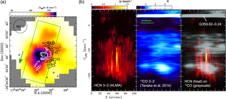
Figure 12. (a) 13CO J = 3–2 integrated intensity map for the −110 to 0 km s−1 velocity range obtained with the ASTE 10 m telescope (Tanaka et al. 2014), with contours of the ALMA J = 3–2 integrated flux density drawn at 5, 10, 20, 50, and 100 Jy beam−1 km s−1. (b) PV diagrams for the ALMA HCN J = 3–2 and ASTE 13CO J = 3–2 data (left and middle panels, respectively) for the rectangular field in panel (a), where the X axis is in the direction of the long side of the rectangle, and the spectra are averaged in the direction of the short side. The bright emission band in the 15–20 km s−1 velocity channels of the 13CO diagram is the foreground infrared dark cloud G359.62−0.24. The HCN and 13CO images are overlaid in the rightmost panel.
Download figure:
Standard image High-resolution imageThis CCC hypothesis is strengthened by the detection of the V-shaped PV pattern across the width of the −80 km s−1 filament. Theoretical studies of CCC systems of two nonidentical clouds (Habe & Ohta 1992; Anathpindika 2010; Takahira et al. 2014) predict the formation of bow shocks inside the larger cloud. If the same model is applicable to a collision between a narrow filament and an extended cloud, the shocked region should have a V-shaped PV pattern when the collision interface is observed in the face-on geometry. We show a schematic illustration of such a collision of the −80 km s−1 filament and the −40 km s−1 cloud in Figure 13. The central portion of the −40 km s−1 cloud is dragged along by the plunging −80 km s−1 filament and the bow shock, while the motion of the outer part of the −40 km s−1 cloud remains less affected. As the intrinsic velocity widths in the pre-collision clouds are smaller than the line-of-sight collision velocity, this gas kinematics is expected to be observed as a V-shaped velocity pattern when viewed along the collision axis (Takahira et al. 2014; Haworth et al. 2015b; Torii et al. 2017). Similar models have been proposed for the formation of half cavities in the Brick cloud, the Sgr B2 complex, and the 50 km s−1 cloud (Higuchi et al. 2014; Tsuboi et al. 2015a, 2015b).

Figure 13. Schematic illustration of a collision between −40 km s−1 cloud and the −80 km s−1 filament, based on theoretical calculations of a CCC system with two dissimilar clouds (Habe & Ohta 1992; Anathpindika 2010; Takahira et al. 2014). (a) The −80 km s−1 filament and the −40 km s−1 cloud immediately before the collision. (b) Same as (a) but in a cross-section view. (c) The collision phase. The central portion of the −40 km s−1 cloud is pushed forward by the −80 km s−1 filament, while the outer part remains undisturbed.
Download figure:
Standard image High-resolution imageThe CCC model also explains the mechanism responsible for heating the −80 km s−1 filament to the observed high temperature. By balancing the heating produced by dissipation of the velocity dispersion of 10 km s−1 in the knots against the radiative cooling by gas and dust (Ao et al. 2013), we obtain 220 K for the gas temperature, where we used velocity gradient dv/dr = 2 × 10² km s−1 pc−1, filament width L = 0.1 pc, and  = 106 cm−3 for the calculation. This temperature is within the parameter range obtained from the non-LTE analysis of the multitransition methanol lines.
4.3. Other Hypotheses
Ravi et al. (2017) proposed a CCC hypothesis that is different from ours, in which the infrared dark cloud G359.62−0.24 is assumed to have fallen from the Galactic halo and collided with CO−0.4. However, PV patterns indicative of physical interactions between G359.62−0.24 and CO−0.4 are not identified in the ALMA HCN J = 3–2 data (Figure 1(a)) nor in the single-dish 13CO data (Figure 12). The parallax measurement toward a water maser source in G359.62−0.24 (Iwata et al. 2017) suggests that the source is most likely in the foreground spiral arm region.
Another hypothesis by Yalinewich & Beniamini (2017), assuming SN–cloud interactions as the origin of the HVCCs, does not conflict with our CCC scenario. As we have shown in a previous paper (Tanaka et al. 2014), CO−0.4 is located on the rim of an expanding-shell-like structure of dense molecular gas with diffuse radio continuum emission, which could be understood as an SN-driven shell. This expanding shell is a plausible candidate of the trigger of the CCC event at CO−0.4.
4.4. CCCs in the GC Region
The large-scale CO surveys toward the CMZ have detected approximately 100 HVCCs and HVCC-like broad-line features (Oka et al. 2012; Tokuyama et al. 2017). Signatures of CCC similar to those found in CO−0.4 have been detected in another archetypical HVCC, CO−0.30–0.07 (Tanaka et al. 2015). If a significant fraction of the HVCCs in the CMZ are CCC sites similar to those archetypical HVCCs, it would indicate a high CCC frequency in the CMZ, since HVCCs are rather short-lived features. By naively assuming that every HVCC indicates one CCC event, the CCC frequency can be estimated from the number of HVCCs, and the duration of the HVCC phase, τHVCC. On ignoring radiative disruption induced by star formation (SF) activity (Haworth et al. 2015a), we obtain τHVCC ∼ r/σv = 7 × 10⁴ year, where r = 1 pc and σv = 15 km s−1 are typical size and velocity dispersion for an HVCC, respectively. Given that a typical cloud mass in the CMZ is ∼104 M⊙ (Miyazaki & Tsuboi 2000) and that the total cloud mass of the CMZ is 3 × 10⁷ M⊙ (Molinari et al. 2011), the CCC frequency is estimated to be 3 per cloud in one orbital period (6 Myr; Sofue 2013). The actual CCC frequency could be somewhat higher, since whether a CCC system is detectable as a broad emission feature may depend on the viewing angle; Haworth et al. (2015b) estimate the detection efficiency to be 20%–30% due to this effect. In total, the CCC rate is roughly estimated to be an order of 1–10 per cloud per orbital period, if CCC is the primary origin of the HVCCs. This is in good agreement with the theoretically predicted CCC frequency: a few to 15 times per orbital period (Tan 2000; Tasker & Tan 2009; Dobbs et al. 2015). Although these theoretical calculations are not necessarily tuned for the GC environment (Dobbs et al. 2015), it is unlikely that the CCC frequency in the CMZ is lower than in the Galactic disk. The high volume filling factor of dense gas, fast orbital velocities, and frequent SN explosions may further increase the CCC frequency.
CCC-triggered SF is among the popular theories for the formation of the massive clusters in the CMZ (Hasegawa et al. 1994; Stolte et al. 2008). Our analysis has shown that  in the post-shock region is ≳106 cm−3, which is approximately two orders of magnitude higher than the average
  in CMZ clouds. This indicates that CCC is actually able to compress the gas to densities typical of star-forming cores during the dynamical time of a collision. However, direct evidence has not been obtained for current SF in CO−0.4; the compact continuum source MM1 is likely to be in the foreground Galactic disk cloud and not associated with CO−0.4. Radio continuum sources indicative of H ii regions are not detected in existing centimeter-wavelength images (e.g., Liszt & Spiker 1995). Although the bright methanol spots on the −80 km s−1 filament are similar to hot cores, their high temperature and rich abundances of complex organic molecules (COMs) could also be an immediate result of a shock passage. Indeed, the fractional methanol abundance of 10−7 is approximately equal to the average value for non-star-forming clouds in the CMZ (Requena-Torres et al. 2006), where the high COM abundance is thought to be maintained by mechanical sputtering of dust mantles, not by thermal desorption from hot cores.
One explanation for the lack of SF signatures may be that the cloud is at an early phase in a CCC-triggered SF process, in which SF has not yet been activated. Alternatively, it is possible that the collision is nonproductive. CCCs may stabilize clouds by enhancing turbulent pressure, or they may even destroy the clouds if the ram pressure of the collision exceeds the gravitational binding pressure (Habe & Ohta 1992; Tan 2000; Dobbs et al. 2011; Johnston et al. 2014; Kruijssen et al. 2014; Rathborne et al. 2014). The general absence of active SF in the HVCCs and the CCC candidate regions—except for the Sgr B2 complex (e.g., Oka et al. 2012; Rathborne et al. 2014; Higuchi et al. 2014; Tanaka et al.2015)—may indicate that CCCs in the CMZ are predominantly in such a nonproductive regime. Considering that every CMZ cloud may experience more than one CCC during its lifetime, nonproductive CCCs may be a non-negligible mechanism for suppressing the SF efficiency in the GC region (Kauffmann et al. 2017).
5. Summary
We have reanalyzed the ALMA archival data for the HVCC CO−0.4, and have explored the origin of the broad-profiled molecular-line emission of the cloud. In particular, through a careful investigation of the velocity field, we have examined the recently proposed hypothesis that the cloud has been gravitationally kicked by an IMBH. Our main conclusions are summarized below:
- 1.The high-resolution ALMA image of the HCN J = 3–2 line shows that the broad-profiled emission detected with single-dish observations consists of a superposition of multiple velocity components: two narrow line (Δv ∼ 10 km s−1 FWZI) components at vLSR = −80 and −40 km s−1, and a moderately broad (Δv ∼ 25–50 km s−1) emission component at −60 km s−1.
- 2.A major fraction of the cloud mass is concentrated in a straight filament with an approximately constant velocity of −80 km s−1. This −80 km s−1 filament intersects the −40 km s−1 clouds at two positions on the plane of the sky (knots A and B), where the velocity width is the largest in the entire cloud. The −80 and −40 km s−1 emissions are smoothly bridged in the PPV space at the knots, forming V-shaped PV patterns across in the direction crossing the filament. The moderately broad-line emission of the −60 km s−1 component almost exclusively appears in these features with "V"-letter-shaped PV patterns.
- 3.The coherent stream structure predicted by the IMBH hypothesis of Oka et al. (2016) is not detected. The steep velocity gradient obtained in the single-dish images, which forms the basis for their model, is found instead to be a beam-smeared feature resulting from the superposition of multiple velocity components. In addition, the gravitationally kicked cloud feature with a 110 km s−1 velocity width reported by Oka et al. (2017) is not reproduced in our reanalysis of the same ALMA data. Instead, this feature is highly likely to be an artifact due to the blurring of spectra caused by the omission of temporal drift of the Doppler-shifted topocentric sky frequencies due to the orbital motion of the Earth.
- 4.The spectral index of the IMBH candidate source MM1/CO−0.40–0.22* is found to be α = 3.0 ± 0.4 from the fluxes at 230 and 265 GHz, which is consistent with a recently reported value of α ≳ 2 measured with 34.25 GHz observations (Ravi et al. 2017). The shallow α of 1.18 ± 0.65 reported by Oka et al. (2017) is most likely due to larger contamination by background emission in the 230 GHz flux measurement. As a molecular-line counterpart is detected at vLSR = 15 km s−1, this source is likely to be a thermal dust emission from the foreground cloud G359.62−0.24 in the Galactic disk.
- 5.The PV structure of CO−0.4 agrees well with that predicted for a collision between two dissimilar-sized clouds; the broad emission component at −60 km s−1 corresponds to the bridging emission that represents the shocked gas layer created by a collision between the −80 and −40 km s−1 components. The portion of the −40 km s−1 cloud that interacts with the narrow −80 km s−1 filament is compressed and dragged in the direction of the relative motion of the filament, creating the V-shaped PV pattern across the filament width.
- 6.None of the evidence previously reported for the IMBH hypothesis is confirmed by this reanalysis. Instead, we argue that a CCC scenario is the most plausible hypothesis for the origin of CO−0.4. If the ∼100 HVCCs detected in wide-field survey maps are predominantly sites of CCCs, we obtain a high CCC frequency of the order of 1–10 per cloud per orbital period.
- 7.We have measured the volume density of the post-shock gas to be ≳106 cm−3 from a non-LTE analysis of multitransition methanol lines. This indicates that a CCC shock can increase the gas density by two orders of magnitude during the dynamical timescale of a collision. Direct evidence for on-going SF in CO−0.4 has not been obtained. The general absence of the SF signatures in HVCCs may indicate that they are still at an early phase of CCC-triggered SF, or that CCCs are nonproductive in the GC region. If the latter is the case, the frequent CCC may contribute to suppress the SF efficiency in the CMZ.
The author is grateful to the anonymous referee, whose suggestions and comments helped to improve the paper. This work was supported by JSPS KAKENHI Grant Number 16K17666. This paper makes use of the following ALMA data: ADS/JAO.ALMA#2012.1.00940.S. ALMA is a partnership of ESO (representing its member states), NSF (USA) and NINS (Japan), together with NRC (Canada), MOST and ASIAA (Taiwan), and KASI (Republic of Korea), in cooperation with the Republic of Chile. The Joint ALMA Observatory is operated by ESO, AUI/NRAO, and NAOJ.
Appendix: Dendrogram Analysis
We employed the dendrogram analysis (Rosolowsky et al. 2008) to extract the primary PPV structure of CO−0.4 from the highly complicated HCN J = 3–2 data cube (Section 3.2). Clumps were identified in the data cube that was smoothed into 2.5 km s−1 velocity bins and digitized in units of 3σ intensities (σ = 13 mJy). The tree diagram presented in Figure 14 shows the hierarchical structure of the identified clumps; the nodes in the diagram represent clumps that are defined as isolated closed isosurfaces at given threshold levels, and the vertical branches connecting the nodes mean that the lower-level clumps are split into multiple clumps at the higher threshold levels. Single-node trees growing directly from the ground ("sprouts"; Lee et al. 2014) are omitted in the diagram.

Figure 14. Dendrogram for the clumps identified in the HCN J = 3–2 PPV map. Leaf clumps growing directly from the ground level ("sprouts") are omitted. The thick-lined trees represent the CO−0.4 main body. The colored trees are the six main branches.
Download figure:
Standard image High-resolution image
The thick-lined tree in the diagram represents the main body of CO−0.4. We identified six main branches in this cloud tree, which are colors other than in black in the diagram. The spatial distributions of these six main branches are superposed on the moment-0 map presented in Figure 6(a). Branches 1, 4, and 5 correspond to the southern, northern, and middle parts of the −80 km s−1 filament. Knots A and B are included in Branches 5 and 4, respectively. An image of the basic structure of the cloud was reconstructed by adding the six main branches and their common trunk nodes (indicated by the thick black lines in Figure 14); this procedure removed from the original image minor leaf clumps and emissions not related to the main body of the cloud.